Dynamic Financial Constraints: Distinguishing Mechanism
Design From Exogenously Incomplete Regimes
The MIT Faculty has made this article openly available.
Please share
how this access benefits you. Your story matters.
Citation
Karaivanov, Alexander and Robert M. Townsend. “Dynamic Financial
Constraints: Distinguishing Mechanism Design From Exogenously
Incomplete Regimes.” Econometrica 82, no. 3 (2014): 887–959.
As Published
http://dx.doi.org/10.3982/ecta9126
Publisher
John Wiley & Sons, Inc/Econometric Society
Version
Original manuscript
Citable link
http://hdl.handle.net/1721.1/96134
Terms of Use
Creative Commons Attribution-Noncommercial-Share Alike
Detailed Terms
http://creativecommons.org/licenses/by-nc-sa/4.0/
Dynamic Financial Constraints: Distinguishing Mechanism Design
from Exogenously Incomplete Regimes
Alexander Karaivanov Simon Fraser University
Robert M. Townsend MIT
July, 2013
Abstract
We formulate and solve a range of dynamic models of constrained credit/insurance that allow for moral hazard and limited commitment. We compare them to full insurance and exogenously incomplete financial regimes (autarky, saving only, borrowing and lending in a single asset). We develop computational methods based on mechanism design, linear programming, and maximum likelihood to estimate, compare, and statisti-cally test these alternative dynamic models with financial/information constraints. Our methods can use both cross-sectional and panel data and allow for measurement error and unobserved heterogeneity. We estimate the models using data on Thai households running small businesses from two separate samples. We find that in the rural sample, the exogenously incomplete saving only and borrowing regimes provide the best fit using data on consumption, business assets, investment, and income. Family and other networks help consumption smoothing there, as in a moral hazard constrained regime. In contrast, in urban areas, we find mechanism de-sign financial/information regimes that are decidedly less constrained, with the moral hazard model fitting best combined business and consumption data. We perform numerous robustness checks in both the Thai data and in Monte Carlo simulations and compare our maximum likelihood criterion with results from other metrics and data not used in the estimation. A prototypical counterfactual policy evaluation exercise using the estimation results is also featured.
Keywords: financial constraints, mechanism design, structural estimation and testing
We are grateful to the coeditor, J-M. Robin and two anonymous referees for their incredibly helpful comments. We also thank H. Cole, L. Hansen, A. Hortacsu, P. Lavergne, E. Ligon, T. Magnac, D. Neal, W. Newey, W. Rogerson, S. Schulhofer-Wohl, K. Wolpin, Q. Vuong, and audiences at Berkeley, Chicago, Duke, MIT, Northwestern, Penn, Toulouse, Stanford, UCSB, the SED conference, the European Meeting of the Econometric Society, and the Vienna Macroeconomics Workshop for many insightful comments and suggestions. Financial support from the NSF, NICHD, SSHRC, the John Templeton Foundation and the Bill and Melinda Gates Foundation through a grant to the Consortium on Financial Systems and Poverty at the University of Chicago is gratefully acknowledged.
1
Introduction
We compute, estimate, and contrast the consumption and investment behavior of risk averse households running small non-farm and farm businesses under alternative dynamic financial and information environments, including exogenously incomplete markets settings (autarky, savings only, non-contingent debt subject to natural borrowing limit) and endogenously constrained settings (moral hazard, limited commitment), both relative to full insurance. We analyze in what circumstances these financial/information regimes can be distinguished in consumption and income data, in investment and income data or in both, jointly. More generally, we propose and apply methods for structural estimation of dynamic mechanism design models. We use the estimates to statistically test the alternative models against each other with both actual data on Thai rural and also urban households and data simulated from the models themselves. We conduct numerous robustness checks, including using alternative model selection criteria and using data not used in the estimation in order to compare predictions at the estimated parameters and to uncover data features that drive our results. We also provide an example of how our estimation method and results could be used to evaluate policy counterfactuals within the model.
With few exceptions the existing literature maintains a dichotomy, also embedded in the national accounts: households are consumers and suppliers of market inputs, whereas firms produce and hire labor and other factors. This gives rise, on the one hand, to a large literature which studies household consumption smoothing. On the other hand, the consumer-firm dichotomy gives rise to an equally large literature on investment in which, mostly, firms are modeled as risk neutral maximizers of expected discounted profits or dividends to owners. Here we set aside for the moment the issues of heterogeneity in technologies and firm growth and focus on a benchmark with financial constraints, thinking of households as firms generating investment and consumption data, as they clearly are in the data we analyze.
The literature that is closest to our paper, and complementary with what we are doing, features risk averse households as firms but largely assumes that certain markets or contracts are missing.1 Our methods might indicate how to build upon these papers, possibly with alternative assumptions on the financial underpinnings. Indeed, this begs the question of how good an approximation are the various assumptions on the financial markets environment, different across the different papers. That is, what would be a reasonable assumption for the financial regime if that part too were taken to the data? Which models of financial constraints fit the data best and should be used in future, possibly policy-informing, work and which are rejected and can be set aside? The latter, though seemingly a more limited objective, is important to emphasize, as it can be useful to narrow down the set of alternatives that remain on the table without falling into the trap that we must definitely pick one model.
Relative to most of the literature, the methods we develop and use in this paper offer several advantages. First, we solve and estimate fully dynamic models of incomplete markets – this is computationally challenging but captures the complete, within-period and cross-period, implications of financial constraints on consumption, investment, and production. Second, our empirical methods can handle any number or type of financial regimes with different frictions. We do not need to make specific functional form or other assumptions to nest those various
1For example, Cagetti and De Nardi (2006) follow Aiyagari (1994) in their study of inequality and assume that labor income is stochastic and uninsurable, while Angeletos and Calvet (2006) and Covas (2006) in their work on buffer stock motives and macro savings rates feature uninsured entrepreneurial risk. In the asset pricing vein, Heaton and Lucas (2000) model entrepreneurial investment as a portfolio choice problem, assuming exogenously incomplete markets in the tradition of Geanakoplos and Polemarchakis (1986) or Zame (1993).
regimes – the Vuong model comparison test we use does not require this. Third, by using maximum likelihood, as opposed to reduced-form techniques or estimation methods based on Euler equations, we are in principle able to estimate a larger set of structural parameters than, for example, those that appear in investment or consump-tion Euler equaconsump-tions and also a wider set of models. More generally, the MLE approach allows us to capture more dimensions of the joint distribution of data variables (consumption, income, investment, capital), both in the cross-section or over time, as opposed to only specific dimensions such as consumption-income comovement or cash flow/investment correlations. Fourth, on the technical side, compared to alternative approaches based on first order conditions, our linear programming solution technique allows us to deal in a straightforward yet extremely general way with non-convexities and non-global optimization issues common in endogenously incomplete mar-kets settings. We do not need to assume that the first order approach is valid or limit ourselves to situations where it is, assume any single-crossing properties, or adopt simplifying adjacency constraints. Combining linear pro-gramming with maximum likelihood estimation allows for a natural direct mapping between the model solutions, already in probabilistic form, and likelihoods which may be unavailable using other solution or estimation meth-ods. Our approach is also generally applicable to other dynamic discrete choice decision problems by first writing them as linear programs and then mapping the solutions into likelihoods.
In this paper we focus on whether and in what circumstances it is possible to distinguish financial regimes, depending on the data used. To that end we also perform tests in which we have full control, that is we know what the financial regime really is by using simulated data from the model. Our paper is thus both a conceptual and methodological contribution. We show how all the financial regimes can be formulated as linear programming problems, often of large dimension, and how likelihood functions, naturally in the space of probabilities/lotteries, can be estimated. We allow for measurement error, the need to estimate the underlying distribution of unobserved state variables, and the use of data from transitions, before households reach steady state.
We apply our methods to a featured emerging market economy – Thailand – to make the point that what we offer is a feasible, practical approach to real data when the researcher aims to provide insights on the source and nature of financial constraints. We chose Thailand for two main reasons. First, our data source (the Townsend Thai surveys) includes panel data on both consumption and investment and this is rare. We can thus see if the combination of consumption and investment data really helps make a difference. Second, we also learn about potential next steps in modeling financial regimes. We know in particular, from other work with these data, that consumption smoothing is quite good, that is, it is sometimes difficult to reject full insurance, in the sense that the coefficient on idiosyncratic income, if significant, is small (Chiappori et al., 2013). We also know that investment is sensitive to income, especially for the poor but, on the other hand, this is to some extent overcome by family networks (Samphantharak and Townsend, 2010). Finally, there is a seeming divergence between high rate-of-return households, who seem constrained in scale, and low rate-of-rate-of-return households, who seemingly should be doing something else with their funds. In short, intermediation is imperfect but varies depending on the dimension chosen.
While we keep these data features in mind, we remain ex-ante neutral in what we expect to find in terms of the best-fitting theoretical model. Hence, we test the full range of regimes, from autarky to full information, against the data. We are interested in how these same data look when viewed jointly though the lens of each of the alternative financial regimes we model. We also want to be assured that our methods, which feature
grid approximations, measurement error, estimation of unobserved distribution of utility promises and transition dynamics, are as a practical matter applicable to actual data. This is our primary intent, to offer an operational methodology for estimating and comparing across different dynamic models of financial regimes that can be taken to data from various sources. We focus on the Thai application, first, but also use Monte Carlo simulations and a variety of robustness checks, including with data or metrics not used in the estimation.
We find that by and large out methods work with the Thai data. In terms of the regime that fits the rural data best, we echo previous work which finds that investment is not smooth and can be sensitive to cash flow fluctuations and that capital stocks are very persistent. Indeed, we find that investment and income data alone are most consistent with the saving only and borrowing and lending regimes, with statistical ties depending on the specification, and this is true as well with the combined consumption and investment data. We also echo previous work which finds that, with income and consumption data alone, full risk sharing is rejected, but not by much, and indeed the moral hazard regime is consistent with these data though sometimes statistically tied with limited commitment or savings only, depending on the specification. We find some evidence that family networks move households more decisively toward less constrained regimes.
In the urban data, we find that the best-fitting financial/information regime is less constraining overall. There is still persistence in the capital stock, though less than in the rural data so, with production data alone, the saving only regime again fits best. But the consumption data is even smoother against income than in the rural sample and the moral hazard and even full insurance regimes fit well, with fewer ties with the more constrained regimes. Overall in the urban data, with combined production and consumption data, moral hazard provides the best fit, unlike in the rural sample. The autarky regime is rejected in virtually all estimation runs with both the rural and urban data.
We are also keen to distinguish across the financial/information regimes themselves, and not their auxiliary assumptions. So in a major robustness check we establish that imposing a parametric production function with estimated parameters does not drive our conclusions. Our primary specification uses unstructured histograms for input/output data, as our computational methods allow arbitrary functional forms. We also perform a range of additional runs with the Thai data that confirm the robustness of our baseline results — imposing risk neutrality, fixing the size of measurement error across regimes, allowing for quadratic adjustment costs in investment, run-ning on data purged from household or year fixed effects, different grid sizes, different distributional assumptions on the unobservable state variable, and alternative assets and income definitions.
In another important robustness check, we perform Monte Carlo estimations with data simulated from the model. In these runs we know what the financial regime really is, and what the true parameter values really are, but we run our estimation the same way as in the Thai data, as if we did not have this information. We find that our ability to distinguish between the regimes naturally depends on both the type of data used and the amount of measurement error. With low measurement error, we are able to distinguish between almost all regime pairs and recover the true regime. As expected, however, higher measurement error in the simulated data reduces the power of the model comparison test – some counterfactual regimes cannot be distinguished from the data-generating baseline and from each other. For example, using investment, assets and income data, we cannot distinguish between the regimes (with the exception of autarky) when moral hazard generated the data. Using joint data on consumption, investment, business assets, and income, however, does markedly improve
the ability to distinguish across the regimes, including with high measurement error in the simulated data. We also incorporate intertemporal data from the model, which we also find to significantly improve our ability to distinguish the regimes relative to when using cross-sections of the same data variables. We also show that the results with simulated data are robust to various modifications — different sizes of measurement error, different grid and sample sizes, and using data-generating parameters identical to the ones estimated from the Thai data. We also do runs allowing for heterogeneity in productivity, risk aversion and interest rates but then ignoring this in the estimation so that the model is mis-specified. Our results remain robust.
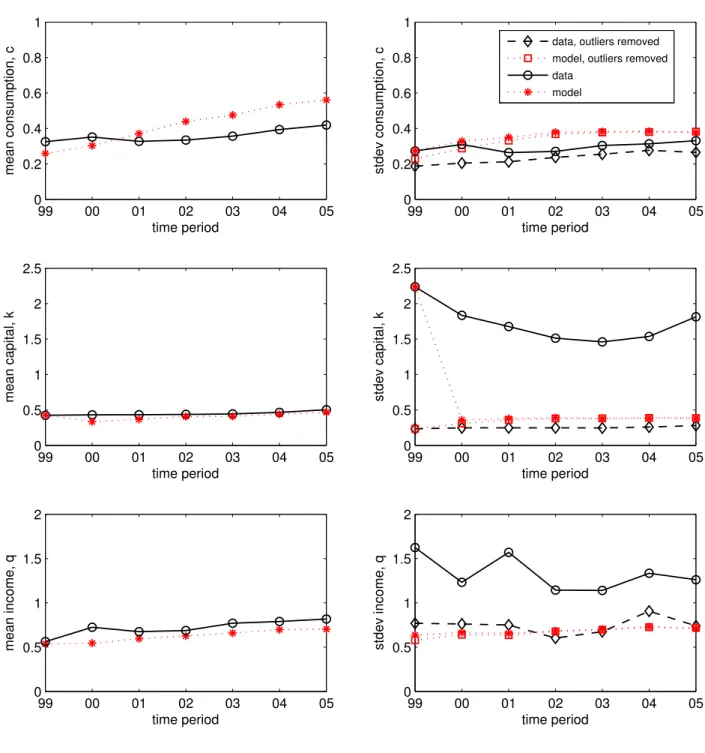
Finally, we look back at some key features of our data and at how the alternative models do in fitting these features and in predicting moments and time paths not used in the estimation. We display the persistence of capital in the data and in the best-fitting financial/information regimes. This helps clarify why the savings-only regime does best when there is substantial persistence (lack of adjustment) as in the rural, and to a less extent the urban, data. We also display the rate of return on assets as a function of assets. Again, the more limited financial regimes (saving only) do best in being consistent with the negative observed relationship in the rural data, i.e., low-asset households have relatively high rates of return and households with higher assets, low rates. The urban data share some features with data simulated from a less constrained regime (moral hazard). We also simulate the time paths of the best-fitting financial regime at the estimated parameters. The means of consumption, business assets, and income fit the Thai data quite well. The standard deviations of these variables also fit, though there is more heterogeneity in the actual than simulated data (removing extreme outliers helps). We also simulate the path for savings in the model and compare, favorably, to financial net worth monthly data which was not utilized in the ML estimation.
In a further robustness check on our likelihood approach and its auxiliary assumptions, a mean squared error metric based on selected moments of the data picks out the savings regime as best fitting in the rural data, which is consistent with our MLE results. The urban data show substantially more smoothing and the ad hoc moments criterion picks out a less constrained regime. We also go beyond the MLE and Vuong tests by running GMM tests based on Euler equations with our data. The Ligon (1998) GMM test using consumption data alone or with business assets or income as instruments shows evidence in favor of either the savings/borrowing or moral hazard regimes, depending on the exact sample or instruments used, in other words, mixed results as in our MLE using consumption and income data alone. The Bond and Meghir (1994) investment sensitivity to cash flow GMM test rejects the null of no financial constraints, as we do in the MLE, but their method is unable to distinguish across the alternative constrained regimes.
Further comparisons to the literature
On the household side, our paper relates to a large literature which studies consumption smoothing.2 On the firm side, there is equally large literature on investment.3 There are also papers attempting to explain stylized facts on firm growth, with higher mean growth and variance in growth for small firms, e.g. Cooley and Quadrini
2
There is voluminous work estimating the permanent income model, the full risk sharing model, buffer stock models (Zeldes, 1989; Deaton and Laroque, 1996) and, lately, models with private information (Phelan 1994; Ligon, 1998) or limited commitment (Ligon, Thomas and Worrall, 2002) among many others.
3
For example, there is the adjustment costs approach of Abel and Blanchard (1983) and Bond and Meghir (1994) among many others. In industrial organization, Hopenhayn (1992) and Ericson and Pakes (1995) model entry and exit of firms with Cobb-Douglas or CES production technologies where investment augments capital with a lag and output produced from capital, labor and other factors is subject to factor-neutral technology shocks.
(2001), among others. Albuquerque and Hopenhayn (2004) and Clementi and Hopenhayn (2006) introduce either private information or limited commitment but maintain risk neutrality.4
In terms of distinguishing across alternative financial constraints, here we set out to see how far we can get, going a bit deeper than most existing literature. For example, the adjustment costs investment literature may be picking up constraints implied by financing and not adjustment costs per se. The ‘pecking order’ investment literature (Myers and Majuf, 1984) simply assumes that internally generated funds are least expensive, followed by debt, and finally equity, discussing wedges and distortions. Berger and Udell (2002) also have a long discussion in this spirit, on small vs. large firm finance. They point out that small firms seem to be informationally opaque yet receive funds from family, friends, angels, or venture capitalists, leaving open the nature of the overall financial regime. Bitler et al. (2005) argue likewise that agency considerations play important role. The empirical work of Fazzari, Hubbard and Petersen (1988) picks up systematic distortions for small firms but, again, the nature of the credit market imperfection is not modeled, leading to criticisms of their interpretation of cash flow sensitivity tests (Kaplan and Zingales, 2000).5
In estimating both exogenously incomplete and endogenous information constrained regimes there are few other similar efforts to which this paper relates. Ligon (1998) uses GMM based on regular vs. inverse Euler equa-tions on Indian villages consumption data to distinguish between a moral hazard model and the permanent income hypothesis assuming CRRA preferences. A similar approach is used in Kocherlakota and Pistaferri (2009) to test between asset pricing implications of a private information model and a standard exogenously incomplete markets model in repeated cross-sections of consumption data from the USA, UK and Italy. Both papers find evidence in favor of the private information model. Meh and Quadrini (2006) compare numerically a bond economy to an economy with unobserved diversion of capital while Attanasio and Pavoni (2011) estimate and compare the extent of consumption smoothing in the permanent income model to that in a moral hazard model with hidden savings (see also Karaivanov, 2012). Krueger and Perri (2011) use data on income, consumption and wealth from Italy (1987-2008) and from the PSID (2004-2006) to compare and contrast the permanent income hypothesis vs. a model of precautionary savings with borrowing constraints and conclude the former explains the dynamics of their data better. Broer (2011) uses a simulated method of moments to estimate stationary joint distributions of consumption, wealth and income in a limited commitment vs. a permanent-income model with US data and finds evidence in favor of the permanent income model, including in a setting with production. Ai and Yang (2007) study an environment with private information and limited commitment. Schmid (2008) is also an effort to esti-mate a dynamic model of financial constraints but by using regressions on model data, not maximum likelihood as here. Dubois et al. (2008) estimate semi-parametrically a dynamic model with limited commitment to explain the patterns of income and consumption growth in Pakistani villages nesting complete markets and the case where only informal agreements are available. Kinnan (2011) tests inverse Euler equations and other implications of moral hazard, limited commitment, and unobserved output financial regimes.
4
Some applied general equilibrium models feature both consumption and investment in the same context, e.g., Rossi-Hansberg and Wright (2007), but there the complete markets hypothesis justifies within the model a separation of the decisions of households from the decisions of firms. Alem and Townsend (2013) provide an explicit derivation of full risk sharing with equilibrium stochastic discount factors, rationalizing the apparent risk neutrality of households as firms making investment decisions.
5Under the null of complete markets there should be no significant cash flow variable in investment decisions, but the criticism is that when the null is rejected, one cannot infer the degree of financial markets imperfection from the magnitude of the cash flow coefficient. One needs to explicitly model the financial regime in order to make an inference, which is what we test here.
Our methods follow logically from Paulson, Townsend and Karaivanov (2006) where we model, estimate, and test whether moral hazard or limited liability is the predominant financial obstacle explaining the observed positive monotonic relationship between initial wealth and subsequent entry into business. Buera and Shin (2013) extend this to endogenous savings decisions in a model with limited borrowing but do not test the micro underpinnings of the assumed regime. Here, we abstract from occupational choice and focus much more on the dynamics as well as include more financial regimes. We naturally analyze the advantages of using the combination of data on consumption and the smoothing of income shocks with data on the smoothing of investment from cash flow fluctuations, in effect filling the gap created by the dichotomy in the literature.
2
Theory
2.1 Environment
Consider an economy of infinitely-lived agents heterogeneous in their initial endowments (assets), k0of a single
good that can be used for both consumption and investment. Agents are risk averse and have time-separable preferences defined over consumption, c, and labor effort, z represented by U (c; z) where U1 > 0; U2 < 0. They
discount future utility using discount factor 2 (0; 1). We assume that c and z belong to the finite discrete sets (grids) C and Z respectively. The agents have access to a stochastic output technology, P (qjz; k) : Q Z K ! [0; 1] which gives the probability of obtaining output/income, q from effort level, z and capital level, k.6 The sets Q and K are also finite and discrete – this could be a technological or computational assumption. Capital, k depreciates at rate 2 (0; 1). Depending on the intended application, the lowest capital level (k = 0) could be interpreted as a ‘worker’ occupation (similar to Paulson et al., 2006) or as firm exit but we do not impose a particular interpretation in this paper.
Agents can contract with a financial intermediary and enter into saving, debt, or insurance arrangements. We characterize the optimal dynamic financial contracts between the agents and the intermediary in different financial markets ‘regimes’ distinguished by alternative assumptions regarding information, enforcement/commitment and credit access. In all financial regimes we study, capital k and output q are assumed observable and verifiable. However, effort, z may be unobservable to third parties, resulting in a moral hazard problem.7
The financial intermediary is risk neutral and has access to an outside credit market with exogenously given and constant over time opportunity cost of funds R.8 The intermediary is assumed to be able to fully commit to
6
We can incorporate heterogeneity in productivity/ability across agents by adding a scaling factor in the production function, as we do in a robustness run in Section 6.2. Note also that q, as defined, can be interpreted as income net of payments for any hired inputs other than z and k:
7
In the working paper version (Karaivanov and Townsend, 2013) we also formulate, compute and perform several estimation runs with a model of hidden output (q is unobservable) and a model of moral hazard and unobserved investment (the capital stock k and effort z are unobservable resulting in a joint moral hazard and adverse selection problem). These regimes have heavier computational requirements than the six featured here, which prevented us from treating them symmetrically in the empirical part. We did find the exogenously incomplete borrowing and saving regimes dominating in the rural data. In the urban data, the hidden output regime fit best in a specification with the parametric production function. Both findings are thus consistent with our main results – exogenously incomplete markets in the rural data and mechanism design financial regimes in the urban data. A more complete summary of these results and the associated mechanism design problems is also available as an online appendix to the current paper at www.sfu.ca/˜akaraiva.
8The assumption of risk neutrality is not essential since there are no aggregate shocks and we can think of the intermediary contracting with a continuum of agents. We perform robustness runs varying the return R, including taking different values at different dates (see Section 6.1) and a run with simulated data varying R in different asset quartiles in the population (see Section 6.2).
the ex-ante (constrained-) optimal contract with agent(s) at any initial state while we consider the possibility of limited commitment by the agents.
Using the linear programming approach of Prescott and Townsend (1984); Phelan and Townsend (1991) and Paulson et al. (2006), we model financial contracts as probability distributions (lotteries) over assigned or implemented allocations of consumption, output, effort, and investment (see below for details). There are two possible interpretations. First, one can think of the intermediary as a principal contracting with a single agent/firm at a time, in which case financial contracts specify mixed strategies over allocations. Alternatively, one can think of the principal contracting with a continuum of agents, so that the optimal contract specifies the fraction of agents of given type or at given state that receive a particular deterministic allocation. It is further assumed that there are no technological links between the agents, the agents cannot collude, and there are no aggregate shocks.9
2.2 Financial and information regimes
We write down the dynamic linear programming problems determining the (constrained) optimal contract in many alternative financial and information regimes which can be classified into two groups. The first group are regimes with exogenously incomplete markets: autarky (A), saving only (S), and borrowing and lending (B). To save space we often use the abbreviated names supplied in the brackets. In these regimes the feasible financial contracts take a specific, exogenously given form (no access to financial markets, a deposit/storage contract, or a non-contingent debt contract, respectively).
In the second group of financial regimes we study, optimal contracts are endogenously determined as solutions to dynamic mechanism-design problems subject to information and incentive constraints. In the main part of this paper we look at two such endogenously incomplete markets regimes – moral hazard (MH), in which agents’ effort is unobserved but capital and investment are observed, and limited commitment (LC) in which there are no information frictions but agents can renege on the contract after observing the output realization.10 All incomplete-markets regimes are compared the full information (FI) benchmark (the ‘complete incomplete-markets’ or ‘first best’ regime). In Section 5.3 we also consider versions of all regimes in which capital changes are subject to quadratic adjustment costs.
2.2.1 Exogenously incomplete markets Autarky
We say that agents are in (financial) ‘autarky’ if they have no access to financial intermediation – neither borrowing nor saving. They can however choose how much output to invest in capital to be used in production vs. how much to consume. The timeline is as follows. The agent starts the current period with business assets (capital) k 2 K which he puts into production. At this time he also supplies his effort z 2 Z: At the end of the period output q2 Q is realized, the agent decides on the next period capital level k0 2 K (we allow downward or
9While conceptually we could allow for aggregate shocks by introducing another state variable in our dynamic linear programs and still be able to solve them using our method, this would increase computational time beyond what is currently feasible at the estimation stage. We perform robustness estimation runs with data with removed year fixed effects to allow for possible common shocks and find almost identical results to the baseline results (see Section 6.1).
10
Again, see footnote 7. The proofs that the optimal contracting problems can be written in recursive form and that the revelation principle applies follow from Phelan and Townsend (1991) and Doepke and Townsend (2006) and hence are omitted.
upward capital adjustments), and consumes c (1 )k + q k0. Clearly, k is the single state variable in the
recursive formulation of the agent’s problem which is relatively simple and can be solved by standard dynamic programming techniques. However, to be consistent with the solution method that we use for the mechanism-design financial regimes where non-linear techniques may be inapplicable due to non-convexities introduced by the incentive and truth-telling constraints (more on this below), we formulate the agent’s problem in autarky (and all others) as a dynamic linear programming problem in the joint probabilities (lotteries) over all possible choice variables allocations (q; z; k0) 2 Q Z K given state k,
v(k) = max
(q;z;k0jk)
X
q;z;k0
(q; z; k0jk)[U((1 )k + q k0; z) + v(k0)] (1)
The maximization of the agent’s value function, v(k) in (1) is subject to a set of constraints on the choice variables, .11 First,8k 2 K the joint probabilities (q; z; k0jk) have to be consistent with the technologically-determined probability distribution of output, P (qjz; k):
X
k0
(q; z; k0jk) = P (qjz; k)X
q;k0
(q; z; k0jk) for all (q; z) 2 Q Z (2)
Second, given that the (:)’s are probabilities, they must satisfy (q; z; k0jk) 0 (non-negativity) 8(q; z; k0) 2 Q Z K, and ‘adding-up’,
X
q;z;k0
(q; z; k0jk) = 1 (3)
The policy variables (q; z; k0jk) that solve the above maximization problem determine the agent’s optimal effort and output-contingent investment in autarky for each k.
Saving only / Borrowing
In this setting we assume that the agent is able to either only save, i.e., accumulate and run down a buffer stock, in what we call the saving only (S) regime; or borrow and save through a competitive financial intermediary – which we call the borrowing (B) regime. The agent thus can save or borrow in a risk-free asset to smooth his consumption or investment in Bewley-Aiyagari manner, in addition to what he could do via production and capital alone under autarky. Specifically, if the agent borrows (saves) an amount b, then next period he has to repay (collect) Rb, independent of the state of the world. Involuntary default is ruled out by assuming that the principal refuses to lend to a borrower who is at risk of not being able to repay in any state (computationally, we assign a high utility penalty in such states). By shutting down all contingencies in debt contracts we aim for better differentiation from the mechanism design regimes.
Debt/savings b is assumed to take values on the finite grid B. By convention, a negative value of b represents savings, i.e., in the S regime the upper bound of the grid B is zero, while in the B regime the upper bound is positive. The lower bound of the grid for b in both cases is a finite negative number. The autarky regime can be subsumed by setting B = f0g. This financial regime is essentially a version of the standard Bewley model
11
In (1) and later on in the paper K under the summation sign refers to summing over k0and not k and similarly for w0and the set W below.
with borrowing constraints defined by the grid B and an endogenous income process defined by the production function P (qjk; z).
The timeline is as follows: the agent starts the current period with capital k and savings/debt b and uses his capital in production together with effort z: At the end of the period, output q is realized, the agent repays/receives Rb, and borrows or saves b0 2 B: He also puts aside (invests in) next period’s capital, k0 and consumes c (1 )k + q + b0 Rb k0: The two ‘assets’ k and b are assumed freely convertible into one another.
The problem of an agent with current capital stock k and debt/savings level b in the S or B regime can be written recursively as:
v(k; b) = max
(q;z;k0;b0jk;b)
X
q;z;k0;b0
(q; z; k0; b0jk; b)[U((1 )k + q + b0 Rb k0; z) + v(k0; b0)] (4)
subject to the technological consistency and adding-up constraints analogous to (2) and (3), and subject to (q; z; k0; b0jk; b) 0 for all (q; z; k0; b0) 2 Q Z K B:
2.2.2 Mechanism Design Regimes Full information
With full information (FI) the principal fully observes and can contract upon agent’s effort and investment – there are no private information or other frictions. We write the corresponding dynamic principal-agent problem as an extension of Phelan and Townsend (1991) with capital accumulation. As is standard in such settings (e.g., see Spear and Srivastava, 1987), to obtain a recursive formulation we use an additional state variable – promised
utility, w which belongs to the discrete set, W . The optimal full-information contract for an agent with current
promised utility w and capital k consists of the effort and capital levels z; k0 2 Z K, next period’s promised utility w0 2 W , and transfers belonging to the discrete set T . A positive value of denotes a transfer from the principal to the agent. The timing of events is the same as in Section 2.2.1, with the addition that transfers occur after output is observed.
Following Phelan and Townsend (1991), the set of promised utilities W has a lower bound, wmin which
corresponds to assigning forever the lowest possible consumption, cmin(obtained from the lowest 2 T and the
highest k0 2 K) and the highest possible effort, zmax 2 Z. The set’s upper bound, wmaxin turn corresponds to
promising the highest possible consumption, cmaxand the lowest possible effort forever:
wF Imin = U (cmin;zmax)
1 and w
F I
max=
U (cmax;zmin)
1 (5)
The principal’s value function, V (k; w) when contracting with an agent at state (k; w) maximizes expected output net of transfers plus the discounted value of future outputs less transfers. We write the mechanism design problem solved by the optimal contract as a linear program in the joint probabilities, ( ; q; z; k0; w0jk; w) over all possible allocations ( ; q; z; k0; w0):
V (k; w) = max
f ( ;q;z;k0;w0jk;w)g
X
;q;z;k0;w0
The maximization in (6) is subject to the ‘technological consistency’ and ‘adding-up’ constraints: X ;k0;w0 ( ; q; z; k0; w0jk; w) = P (qjz; k) X ;q;k0;w0 ( ; q; z; k0; w0jk; w) for all (q; z) 2 Q Z; (7) X ;q;z;k0;w0 ( ; q; z; k0; w0jk; w) = 1, (8)
as well as non-negativity: ( ; q; z; k0; w0jk; w) 0 for all ( ; q; z; k0; w0) 2 T Q Z K W .
The optimal FI contract must also satisfy an additional, promise keeping constraint which reflects the princi-pal’s commitment ability and ensures that the agent’s present-value expected utility equals his promised utility, w:
X
;q;z;k0;w0
( ; q; z; k0; w0jk; w)[U( + (1 )k k0; z) + w0] = w (9)
By varying the initial promise w we can trace the whole Pareto frontier for the principal and the agent. The optimal FI contract is the probabilities ( ; q; z; k0; w0jk; w) that maximize (6) subject to (7), (8) and (9).
The full information contract implies full insurance, so consumption is smoothed completely against output, q (conditioned on effort z if utility is non-separable). It also implies that expected marginal products of capital ought to be equated to the outside interest rate implicit in R, adjusting for disutility of labor effort which the planner would take that into account in determining how much capital k to assign to a project. The intermediary/bank (planner) has access to outside borrowing and lending at the rate R, but internally, within its set of customers it can in effect have them ‘borrow’ and ‘save’ among each other, i.e., take some output away from one agent who might otherwise have put money into his project and give that to another agent with high marginal product. A lot of this nets out so only the residual is financed with (or lent to) the outside market. In contrast, the B/S regime shuts down such within-group transfers and trades and instead each agent is dealing with the market directly.
Moral hazard
In the moral hazard (MH) regime the principal can still observe and control the agent’s capital and investment (k and k0), but he can no longer observe or verify the agent’s effort, z. This results in a moral hazard problem. The state k here can be interpreted as endogenous collateral. The timing is the same as in the FI regime. However, the optimal MH contract ( ; q; z; k0; w0jk; w) must satisfy an incentive-compatibility constraint (ICC), in addition to (7)-(9).12 The ICC states that, given the agent’s state (k; w) and recommended effort level z; capital k0; and transfer ; the agent must not be able to achieve higher expected utility by deviating to any alternative effort level ^
z. That is, 8(z; ^z) 2 Z Z we must have, X ;q;k0;w0 ( ; q; z; k0; w0jk; w)[U( + (1 )k k0; z) + w0] X ;q;k0;w0 ( ; q; z; k0; w0jk; w)P (qj^z; k) P (qjz; k)[U ( + (1 )k k 0; ^z) + w0] (10) 12
For more details on the ICC derivation in the linear programming framework, see Prescott and Townsend (1984). The key term is the ‘likelihood ratio’,P (qP (qj^z;k)
Apart from the additional ICC constraint (10), the MH regime differs from the FI regime in the set of feasible promised utilities, W . In particular, the lowest possible promise under moral hazard is no longer the value wminF I from (5). Indeed, if the agent is assigned minimum consumption forever, he would not supply effort above the minimum possible. Thus, the feasible range of promised utilities, W for the MH regime is bounded by:
wminM H = U (cmin; zmin)
1 and w
M H
max =
U (cmax; zmin)
1 (11)
The principal cannot promise a slightly higher consumption in exchange for much higher effort such that agent’s utility falls below wM Hmin since this is not incentive compatible. If the agent does not follow the principal’s recom-mendations but deviates to zminthe worst punishment he can receive is cminforever.
The constrained-optimal contract in the moral hazard regime, M H( ; q; z; k0; w0jk; w) solves the linear pro-gram defined by (6)–(10). The contract features partial insurance and intertemporal tie-ins, i.e., it is not a repetition of the optimal one-period contract (Townsend, 1982).
Limited commitment
The third setting with endogenously incomplete financial markets we study assumes away private information but focuses on another friction often discussed in the consumption smoothing and investment literatures (e.g., Thomas and Worrall, 1994; Ligon et al., 2000 among others) – limited commitment (LC). As in those papers, by ‘limited commitment’ we mean that the agent may potentially renege on the contract after observing his output realization knowing the transfer he is supposed to give to others through the intermediary. Another possible interpretation of this, particularly relevant for developing economies, is a contract enforcement problem. The maximum penalty for a reneging agent is permanent exclusion from future credit/risk-sharing – i.e., our assumption is the agent goes to autarky forever.
Using the same approach as with the other financial regimes, we write the optimal contracting problem under limited commitment as a recursive linear programming problem. The state variables are capital, k 2 K and promised utility, w2 W . In this model regime the set (here, a closed interval on R) of feasible promised utilities, W is an endogenous object to be iterated over during the dynamic program solution (Abreu, Pearce and Stacchetti, 1990). We initialize the lower bound of W , wLCminas equal to the autarky value at kmin(see Section 2.2.1) and set
the initial upper bound to wmaxLC = wmaxF I . A similar solution approach, including allowing for randomization over allocations, is used in Ligon et al. (2000).
Given the agent’s current state (k; w) the problem of the intermediary is
V (k; w) = max
( ;q;z;k0;w0jk;w)
X
;q;z;k0;w0
( ; q; z; k0; w0jk; w)[q + (1=R)V (k0; w0)]
subject to the promise-keeping constraint X
;q;z;k0;w0
( ; q; z; k0; w0jk; w)[U( + (1 )k k0; z) + w0] = w,
respect-ing our timrespect-ing that effort z is decided before output q is realized,13 X ;k0;w0 ( ;q;z;k0;w0jk;w) P ~;~k0; ~w0 (~;q;z;~k0; ~w0jk;w) U ( + (1 )k k0; z) + w0 (k; q; z) for all (q; z) 2 Q Z (12)
and subject to non-negativity ( ; q; z; k0; w0jk; w) 0, technological consistency and adding-up, X ;k0;w0 ( ; q; z; k0; w0jk; w) = P (qjz; k) X ;q;k0;w0 ( ; q; z; k0; w0jk; w) for all (q; z) 2 Q Z; X ;q;z;k0;w0 ( ; q; z; k0; w0jk; w) = 1,
In constraint (12), (k; q; z) denotes the present utility value of the agent going to autarky forever with his output at hand q and capital k, defined as:
(k; q; z) max
k02K U (q + (1 )k k
0; z) + v(k0)
where v(:) is the autarky regime value function defined in Section 2.2.1.
3
Computation
3.1 Solution Methods
We solve the dynamic programs for all financial regimes numerically. Specifically, we use the linear programming (LP) methods developed by Prescott and Townsend (1984) and applied in Phelan and Townsend (1991) and Paul-son et al. (2006) where, as shown in the previous section, the dynamic problems are written in terms of probability distributions (‘lotteries’). An alternative to the LP method in the literature is the ‘first order approach’ (Rogerson, 1985) whereby the incentive constraints are replaced by their first order conditions.14 The public finance litera-ture in the tradition of Mirrlees has adopted these latter methods to provide elegant characterizations of solutions to tax and insurance problems, or used ex-post verification to show that simplified, less constrained problems can be solved without loss of generality (Abraham and Pavoni, 2008; Farhi and Werning, 2012; Golosov et al., 2006; Golosov and Tsyvinski, 2007; Ai and Yang, 2007). A problem with that approach arises from possible non-convexities induced by the incentive or commitment constraints.15 Here, by way of contrast we operate in extremely general environments, following Fernandes and Phelan (2000) and Doepke and Townsend (2006). Our linear programming approach can be applied for any preference and technology specifications since, by construc-tion, it convexifies the problem by allowing any possible randomization (lotteries) over the solution variables. The only potential downside is that the LP method may suffer from a ‘curse of dimensionality’ due to its use of
13
The terms P ( ;q;z;k0;w0jk;w) ~;~k0 ; ~w0 (~;q;z;~k0; ~w0jk;w)
correspond to the respective probabilities conditional on q; z having been realized. 14
The first order approach requires imposing monotonicity and/or convexity assumptions on the technology (Rogerson 1985; Jewitt, 1988) or, alternatively, as in Abraham and Pavoni (2008), employing a numerical verification procedure to check its validity for the particular problem at hand.
15
We found such non-convexities in some of our solutions for the mechanism design regimes and hence we cannot use the first order approach. See also Kocherlakota (2004).
discrete grids for all variables. However, as shown above, by judicious formulation of the linear programs, this deficiency can be substantially reduced.
To speed up computation, we solve the dynamic programs for each regime using policy function iteration (e.g., see Judd, 1998). That is, we start with an initial guess for the value function, obtain the optimal policy function and compute the new value function that would occur if the computed policy function were used forever. We iterate on this procedure until convergence. At each iteration step, that is for each interim value function iterate, we solve a linear program in the policy variables for each possible value of the state variables.16 In the limited commitment regime, LC (see Section 2), the promised utilities set is endogenously determined and has to be iterated and solved for together with the value function during the solution process, due to the commitment or truth-telling constraints, which makes the LC regime computationally harder than the MH or FI regimes.
3.2 Functional Forms and Grids
Below are the functional forms we adopt in the empirical analysis. They are chosen and demonstrated below to be flexible enough to generate significant and statistically distinguishable differences across the financial regimes. As argued earlier, we can handle in principle any preferences and technology, including with non-convexities but, of course, in practice we are limited by computational concerns (estimation time sharply increases with the number of estimated parameters). We also verify robustness by using different parameterizations and model specifications (see Section 6).
Agent preferences are of the CES form:17
U (c; z) = c
1
1 z
The production function, P (qjz; k) : Z K ! Q represents the probability of obtaining output level, q 2 Q fq1; q2; ::q#Qg; from effort z 2 Z and capital k 2 K. In our baseline runs with Thai data we fit P (qjz; k)
non-parametrically using a histogram function from a subset of households in the rural sample for which we have labor time data.18 In robustness runs (with both the rural and urban data) we also use a parametric form for P (qjz; k) with parameters we estimate which encompasses production technologies ranging from perfect substitutes to Cobb-Douglas to Leontief forms (see Section 6.1 below for details).
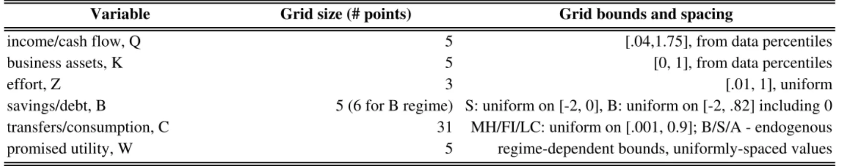
To get an idea of the computational complexity of the dynamic contracting problems we solve, Table 1 shows the number of variables, constraints, and linear programs that need to be solved at each iteration for each regime for the grids we use in the empirical implementation. The number of linear programs is closely related to the grid size of the state variables while the total number of variables and constraints depends on the product of all grid dimensions. The biggest computational difficulties arise from increasing #K or #Z as this causes an exponential
16
The coefficient matrices of the objective function and the constraints are created in Matlab while all linear programs are solved using the commercial LP solver CPLEX version 8.1. The computations were performed on a dual-core, 2.2 Ghz, 2GB RAM machine.
17
Our linear programming solution methodology does not require separable preferences. However, assuming separability is standard in the dynamic contracts literature so we adopt it for comparison purposes. We perform a robustness run with a more general preference form with an additional parameter in Section 6.1.
18
Specifically, we map output, q, assets, k and time worked, z data onto the model grids and set P (qjz; k) equal to the fraction of
observations in each (q; k; z) grid cell. For the baseline runs with urban data, for data availability reasons we used the same data on z but the actual urban sample values for q and k:
increase in the number of variables and/or constraints. This is why we keep these dimensions relatively low, whereas using larger #T (or, equivalently #C) is relatively ‘cheap’ computationally.
The grids that we use in the estimation runs reflect the relative magnitudes and ranges of the variables in the Thai data or simulated data. In our baseline estimation runs we use a five-point capital grid K with grid points corresponding to the 10th, 30th, 50th, 70th and 90th percentiles in the data. The same applies for the output grid Q. The baseline grid for promised utility, W consists of five uniformly-spaced points over the respective bounds for the MH, FI or LC regimes. Table 2 displays the grids we use in the estimation runs with Thai rural data. Further specific details on how all grids are determined are given in Section 5.2. We can use (and do robustness runs with) finer grids but the associated computational time cost is extremely high at the estimation stage because of the need to compute the linear programs and iterate at each parameter vector during the estimation. This is why we keep dimensions relatively low at present.
4
Empirical Method
In this section we describe our estimation strategy. We estimate via maximum likelihood each of the alternative dynamic models of financial constraints developed in Section 2. Our basic empirical method is as follows. We write down a likelihood function that measures the goodness-of-fit between the data and each of the alternative model regimes. We then use the maximized likelihood value for each model (at the MLE estimates for the parameters) and perform a formal statistical test (Vuong, 1989) about whether we can statistically distinguish between each pair of models relative to the data. We thus approach the data as if agnostic about which theoretical model fits them best and let the data themselves determine this. The results of the Vuong test, a sort of ‘horse race’ among competing models, inform us which theory(ies) fits the data best and also which theories can be rejected in view of the observed data.
This is a structural estimation and model comparison paper, and so naturally this poses the question of dis-tinguishing between testing or rejecting the imposed model structure (functional and parametric forms) versus testing the actual relationships between the features we are interested in (the financial and information regimes). In all structural MLE runs these two dimensions are tested jointly by construction. We try to deal with this issue in several ways. First, in the robustness Section 6 we explore some alternative functional forms or parameterizations and perform the empirical analysis for different data samples and variable definitions. Runs with data simulated from the model are also performed to test the validity of our estimation method. Second, in section 7 we sup-plement the maximum likelihood and Vuong test results with additional graphs, tables and alternative criteria of fit to better illustrate and provide further supporting evidence for the robustness of the main results. Finally, we use flexible and standard functional forms for preferences and the unobservable states distribution which are held constant across the alternative regimes, that is, any differences in likelihood are due to the nature of financial constraints imposed by the model, not due to differences in functional forms.
The financial regimes we study have implications for both the transitional dynamics and long-run distributions of variables such as consumption, assets, investment, etc. Given our application to Thailand – an emerging, rapidly developing economy, we take the view that the actual data is more likely to correspond to a transition than to a
steady state.19 Thus, estimating initial conditions (captured by the initial state variables distribution) is important for us, as well as fitting the subsequent trajectories using intertemporal data. In addition, our simulations show slow dynamics for the model variables in the mechanism design regimes and, theoretically, some regimes can theoretically have degenerate long-run distributions (e.g., ‘immiseration’ in the moral hazard model). These are further reasons to focus on transitions instead of steady states in the estimation. We explain the details below.
4.1 Maximum likelihood estimation
Suppose we have panel data f^xjtgn;j=1;t=1T where j = 1; :::n denotes sample units and t denotes time (in our
application sample units are households observed over seven years). The data are assumed i.i.d. across households, j. In this paper we use various subsets of data collected from rural and urban Thai households running small businesses on their productive assets, consumption and income,f^kjt; ^cjt; ^qjtg where t = 0; :::; 6 correspond to the
years 1999-2005. We also construct investment data as ^{jt k^jt+1 (1 )^kjt for t = 0; :::; 5. See Section 5.1
for more details.
For each household j, call ^yj the vector of variables used in the MLE. In the various runs we do this vector
can consist of different cross-sectional variables (e.g., t = 0 consumption and income; that is ^yj = (^cj0; ^qj0) or
t = 6 consumption, income, investment and capital; that is ^yj = (^cj6; ^qj6; ^{j6; ^kj6)) or can consist of variables
from different time periods (e.g., consumption and income at t = 0 and t = 1; that is ^yj = (^cj0; ^qj0; ^cj1; ^qj1)).
The data ^y may contain measurement error. Assume the measurement error is additive and distributed N (0; ( me (x))2) where (x) denotes the range of the grid X for variable x, i.e., (x) xmax xmin where
x is any of the variables used in the estimation (e.g., consumption). The reasoning is that for computational time reasons we want to be as parsimonious with parameters as possible in the likelihood routine while still allowing the measurement error variance to be commensurate with the different variables’ ranges. In principle, more com-plex versions of measurement error can be introduced at the cost of computing time. The parameter me will be
estimated in the MLE.
Call s1 the vector of observable state variables and s2 the vector of unobservable state variables. We have s1 = k for all models while s2 = w or s2 = b or s2 absent, depending on the financial regime. In the estimation runs that follow there are two cases depending on whether or not the set of variables, y used in the estimation includes s10– the initial values of the observed state. Call y1 yns10, i.e., all variables in y which are not s10. For example, in the runs with y = (c0; q0) data in Sections 5 and 6 below, we have y = y1since k0= s10is not among
the variables y, while in the runs with y = (k0; i0; q0) data we have y 6= y1since k0 = s10is among the variables
y used in the estimation (see below for more discussion on this).
1. Model solutions and joint probabilities
For each possible values of the state variables, s1 and s2 over the grids S1 and S2 in a given model regime (e.g., k; w – the capital stock and promised utility for the MH, FI or LC models) and given structural parameters s in the preferences and technology functions, the model solution obtained from the respective linear program (see Section 2) is a discrete joint probability distribution, (:js1; s2). For example, the MH model solution consists of the joint probabilities ( ; q; z; k0; w0jk; w). Using the LP solution (:js1; s2), we can easily obtain, essentially
19
We do a robustness estimation run in Section 6.2 with simulated data drawn after running the model a large number of periods, approximating a steady state.
by summing over the different variables and probabilities (see Appendix A for more details), the theoretical joint probability distribution in model m over any set of variables y1used in the MLE – for instance, y1could be t = 0 consumption and income (c0; q0). Call this probability distribution gm(y1js1; s2; s).
2. Initialization of observable and unobservable state variables
Let h(s10; s20; d) denote the initial discrete joint distribution of the state variables over their corresponding grids, the parameters of which, d will be estimated in the MLE. To initialize the observed state variable s1 (capital k in all models) we take the actual dataf^kjgnj=1for the initial period used in the estimation and discretize
it over the grid K via histogram function. Call the resulting discrete probability distribution h(s10) – the marginal distribution of s10.20 The initial values of the unobservable state s2
0(b or w, depending on the regime) are treated as
a source of unobserved heterogeneity. Their distribution and possible dependence on s10 are parametrized by d. In our baseline estimation runs with the Thai data in Section 5 we assume that the initial distributions of the state variables s1 and s2 are independent.21 We relax this assumption in robustness runs (see Section 6.1 and Table 9), where we allow the initial unobserved state s20 (e.g., initial promised utility) to be correlated with the initial distribution of s10(initial assets) via an additional estimated parameter. Note that we do not assume that the states s1and s2 are independent beyond the initial period – they evolve endogenously with the model dynamics.
3. The likelihood
To form the likelihood of model m with observations from variables y (e.g., consumption and income), de-note by hm(y1; s10js20; s) the joint density of all observables conditional on all unobservables. Then, ‘integrate’ over the initial distribution of the unobservable state, i.e., formP
s2
0
hm(y1; s10js20; s)h(s20; d) where h(s20; d) is the marginal distribution of s20. In our baseline specification with independent initial states s10 and s20, we have h(s20; d) = (s02; d) and the summation over s20is done using a histogram function over the grid S2(e.g., W in the MH model). Naturally, since the only state in autarky (k) is observable, this step is not performed when we estimate the A model. We have
P s2 0 hm(y1; s10js02; s)h(s20; d) =P s2 0 gm(y1js10; s20; s)h(s10js20)h(s20; d) = (13) = P s2 0 gm(y1js10; s20; s)h(s10; s20; d) fm(y1; s10; s; d)
Above, fm(y1; s10; s; d) is the joint distribution of y1 and s10 in model m given parameters s; d. For in-stance, this could be the theoretical joint distribution of c,q,i, and k in the MH model for initial state distribution h(s10; s20; d) over the grid K W . In the runs in which s10 is not among the variables y used in the MLE (e.g., the runs with c,q data), we further ‘integrate out’ the initial distribution of the observable state to obtain the joint
20
In constructing the discrete initial distribution h(s10) (or h(s10; s20) in general) we allow for the possibility that the ^k data contain
measurement error, with the same additive Normal specification parametrized by me assumed above. We use essentially the method described in (15) below to compute the probability mass at each grid point. This step is done upfront since we need the discretized distribution h(s10; s20) to obtain using the LP solution the joint distribution of the variables y1used in the MLE (see fmand Fmbelow).
21
Specifically, in these runs we assume that the unobserved state w in the MH, FI, LC models is distributed (s20; d) = N ( w; 2 w)
and the unobserved state b in the B and S models is distributed (s2
0; d) = N ( b;
2
b). Thus, in the independence case we have
h(s10; s20; d) = h(s10) (s20; d). Assuming Normality of the initial b or w distributions is not essential for our method and more general
distributional assumptions can be incorporated at the computational cost of additional estimated parameters. We perform a robustness run with a Gaussian mixture distribution in Section 6.1.
distribution in model m of the variables y, fm(y; s; d) =P s1 0 P s2 0 gm(y1js10; s20; s)h(s10; s20; d) (14)
We also allow for measurement error in the variables in y1. Let (:j ; ) denote the pdf of N ; 2 . Given the assumed measurement error distribution, the likelihood of observing data ^y1j (for instance ^cj; ^qj), relative to
any grid point y1r 2 Y1, for any r = 1; :::; #Y1 is: L
Y
l=1
^
y1;lj jy1;lr ; l( me) (15)
where l = 1; :::; L indexes the different elements of y1 or ^y1 (e.g., L = 2 for y1 = (c; q)) and where l(
me) =
me (yl) is the measurement error standard deviation for each variable, as explained earlier.
Focus on the case y = y1; the case y = (y1; s10) is handled analogously but the algebra is more cumber-some since for each j we need to condition on its s10 value in the grid S1. Expression (15) implies that the likelihood of observing data vector ^yj (consisting of L data variables indexed by l) for model m, at parameters
( s; d; me) and initial states distribution h(s10; s20; d) is
Fm(^yj; ) #Y X r=1 fm(yr; s; d) L Y l=1 ^ yjljyrl; l( me) (16)
where fm(yr; s; d) is the value of (14) at yr, i.e., the probability mass which model m puts on grid point r,
and where we assume that measurement errors in all variables are independent from each other. We basically sum over all grid points, appropriately weighted by fm, the likelihoods in (15). For example, for cross-sectional consumption and income data ^yj = (^yj1; ^yj2) = (^cj; ^qj), we have
Fm(^cj; ^qj; ) =
X
r
fm((c; q)r; s; d) ^cjjcr; 1( me) q^jjqr; 2( me)
where r goes over all elements of the joint grid C Q, r = 1; :::; #C#Q and where l = 1 in (16) refers to consumption c and l = 2 refers to income q.
Multiplying (16) over the sample units (households) and taking logs, the normalized by n log-likelihood of dataf^yjgnj=1in model m with initial state distribution h(s10; s20; d) at parameters is,
m n ( ) 1 n n X j=1 ln Fm(^yj; ) : (17)
The maximization of the log-likelihood (17) over is performed by an optimization algorithm robust to local maxima.22 Standard errors are computed using bootstrapping, repeatedly drawing with replacement from the data.
22
We first perform an extensive grid search over the parameter space to rule out local extrema and then use non-gradient based opti-mization routines (Matlab’s function patternsearch) to maximize the likelihood.
4.2 Testing and model selection
We follow Vuong (1989) to construct and compute an asymptotic test statistic that we use to distinguish across the alternative models using simulated or actual data. The Vuong test does not require that either of the compared models be correctly specified. The null hypothesis of the Vuong test, is that the two models are asymptotically equivalent relative to the true data generating process – that is, cannot be statistically distinguished from each other based on their ‘distance’ from the data in KLIC sense. The Vuong test-statistic is normally distributed under the null hypothesis. If the null is rejected (i.e., the Vuong Z-statistic is large enough in absolute value), we say that the higher likelihood model is ‘closer to the data’ (in KLIC sense) than the other.
More formally, suppose the values of the estimation criterion being minimized, i.e., minus the log-likelihood, for two competing models are given by L1n(^1) and L2n(^2) where n is the sample size and ^1 and ^2 are the parameter estimates for the two models.23 The test allows us to rank the likelihoods with the data of all studied models pairwise, although this ranking is not necessarily transitive (model A may be preferred to model B, which may be preferred to model C, but A and C can be tied). Define the difference in lack-of fit statistic:
Tn= n 1=2 1 n(^ 1 ) 2n(^2) ^n
where ^n is a consistent estimate of the asymptotic variance, n of the log of the likelihood ratio, 1n(^ 1
)
2
n(^
2
).24 Under regularity conditions (see Vuong, 1989, pp. 309-13 for details), if the compared models are strictly non-nested, the test-statistic Tnis distributed N (0; 1) under the null hypothesis.
5
Application to Thai Data
5.1 DataIn this section we apply our estimation method to actual household-level data from a developing country. We use the Townsend Thai Data, both the rural Monthly Survey and the annual Urban Survey (Townsend, Paulson and Lee, 1997). Constrained by space and computation time, we report primarily on the rural data, but where possible compare and contrast results with the urban data.
The Monthly Survey data were gathered from 16 villages in four provinces, two in the relatively wealthy and industrializing Central region near Bangkok, Chacheongsao and Lopburi, and two in the relatively poor, semi-arid Northeast, Buriram and Srisaket. That survey began in August 1998 with a comprehensive baseline questionnaire on an extensive set of topics, followed by interviews every month. Initially consumption data were gathered weekly, then bi-weekly. All variables were added up to produce annual numbers. The data we use here begins in January 1999 so that technique and questionnaire adjustments were essentially done. We use a balanced panel of
23
For the functional forms and parameter space we use in the estimation, the models we study are statistically non-nested. Formally, following Vuong (1989), if two models are represented by the parametric families of conditional distributionsF = fFYjZ(:; :j 1) : 12
Rd 1
g and G = fGYjZ(:; :j 2) : 2 2 R
d 2
g where fYi; Zigni=1is i.i.d. data, they are non-nested ifF \ G = ?. The Vuong test can
be also used for overlapping models, i.e., neither strictly nested nor non-nested, in which case a two-step procedure is used (see Vuong, 1989, p. 321).
24
531 rural households who run small businesses observed for seven consecutive years, 1999 to 2005.
Consumption expenditures, c include owner-produced consumption (rice, fish, etc.). Income, q is measured on accrual basis (see Samphantharak and Townsend, 2010) though at an annual frequency this is close to cash flow from operations. Business assets, k include business and farm equipment, but exclude livestock and household assets such as durable goods. We do perform a robustness check with respect to the asset definition — see Section 6.1. Assets other than land are depreciated. All data are in nominal terms but inflation was low over this period. The variables are not converted to per-capita terms, i.e., household size is not brought into consideration (though we do a robustness check below). We construct a measure of investment using the assets in two consecutive years as: it kt+1 (1 )ktfor each household.
The monthly data measure transfers and borrowing/lending among households within a village, and so we are able to construct measures of financial networks. Gifts and especially loans are large when they occur, averaging 9% and 60% of household consumption, respectively. From an initial Census we also have the location of parents, siblings, adult children, and parents’ siblings of each surveyed household and his/her spouse, and so we can construct an indicator of family-connected households in each village.
From the Urban Survey which began later, in November 2005, we use a balanced panel of 475 households observed each year in the period 2005 to 2009 from the same four provinces as in the rural data plus two more, Phrae province in the North of Thailand and Satun province in the South. We use the same variables – consumption expenditure, business assets and income as in the rural data though in this case the variables are annual to begin with, so the recall period is different. Note there is an overlap in years for 2005, and we do use that year for comparable estimation results with the rural and urban data.
Table 3 displays summary statistics of these data in thousands Thai baht for both the rural and urban samples (the average exchange rate in the 1999-05 period was 1 USD = 41 Baht). All magnitudes are higher in the urban sample because those households are richer on average. Business assets, k and investment, i are very unequally distributed as reflected in the high standard deviations and ratio between mean and median. There are many observations with zero of close to zero assets and few with quite large assets. More detail is reported in Samphantharak and Townsend (2010, ch. 7) for the monthly data.
Figure 1 plots, for both the urban and rural data, deviations from the sample year averages for income, con-sumption, and investment. As in Townsend (1994), the figure visualizes the relative degree of consumption and investment smoothing relative to income fluctuations. We see that there is significant degree of consumption smoothing in the data, but it is not perfect as the full insurance hypothesis would imply (if all households were identical, the right hand panel should be flat at zero). Investment should not move with cash flow fluctuations either, controlling for productivity, but should move with investment opportunities. This is more so in the urban data.
Figure 2 plots the relationships between consumption level changes and asset level changes each relative to income level changes, as in Krueger and Perri (2011). We sort the data into twenty bins by average income change over the seven years (using quantiles) and report the average consumption and assets change corresponding to each bin (each marker corresponds to a bin). The comovement between consumption changes and income changes, c and q in the figure can be viewed as a measure of the degree of consumption smoothing in the data. For the rural data, the top left panel shows a positive relationship between consumption and income changes (correlation