Rotation of the magnetic field in Earth's magnetosheath by bulk magnetosheath plasma flow

(1)

HAL Id: hal-00317939

https://hal.archives-ouvertes.fr/hal-00317939

Submitted on 7 Mar 2006

HAL is a multi-disciplinary open access

archive for the deposit and dissemination of

sci-entific research documents, whether they are

pub-lished or not. The documents may come from

teaching and research institutions in France or

abroad, or from public or private research centers.

L’archive ouverte pluridisciplinaire HAL, est

destinée au dépôt et à la diffusion de documents

scientifiques de niveau recherche, publiés ou non,

émanant des établissements d’enseignement et de

recherche français ou étrangers, des laboratoires

publics ou privés.

Rotation of the magnetic field in Earth’s magnetosheath

by bulk magnetosheath plasma flow

M. Longmore, S. J. Schwartz, E. A. Lucek

To cite this version:

M. Longmore, S. J. Schwartz, E. A. Lucek. Rotation of the magnetic field in Earth’s magnetosheath

by bulk magnetosheath plasma flow. Annales Geophysicae, European Geosciences Union, 2006, 24

(1), pp.339-354. �hal-00317939�

(2)

SRef-ID: 1432-0576/ag/2006-24-339 © European Geosciences Union 2006

Annales

Geophysicae

Rotation of the magnetic field in Earth’s magnetosheath by bulk

magnetosheath plasma flow

M. Longmore1, S. J. Schwartz2, and E. A. Lucek2

1_{Astronomy Unit, Queen Mary, University of London, London, UK}

2_{Blackett Laboratory, Imperial College London,London, UK}

Received: 27 June 2005 – Revised: 19 December 2005 – Accepted: 20 December 2005 – Published: 7 March 2006

Abstract. Orientations of the observed magnetic field in Earth’s dayside magnetosheath are compared with the predicted field line-draping pattern from the Kobel and Fl¨uckiger static magnetic field model. A rotation of the over-all magnetosheath draping pattern with respect to the model prediction is observed. For an earthward Parker spiral, the sense of the rotation is typically clockwise for northward IMF and anticlockwise for southward IMF. The rotation is consistent with an interpretation which considers the twist-ing of the magnetic field lines by the bulk plasma flow in the magnetosheath. Histogram distributions describing the differences between the observed and model magnetic field clock angles in the magnetosheath confirm the existence and sense of the rotation. A statistically significant mean value of the IMF rotation in the range 5◦₋₃₀◦_{is observed in all}

re-gions of the magnetosheath, for all IMF directions, although the associated standard deviation implies large uncertainty in the determination of an accurate value for the rotation. We discuss the role of field-flow coupling effects and dayside merging on field line draping in the magnetosheath in view of the evidence presented here and that which has previously been reported by Kaymaz et al. (1992).

Keywords. Interplanetary physics (Interplanetary magnetic

fields) – Magnetospheric physics (Magnetopause; Cusp and boundary layers; Magnetosheath)

1 Introduction

In the MHD description of the Sun-Earth interaction, the in-terplanetary magnetic field (IMF) is embedded in the solar wind flow which slows across the bow shock and deflects around the Earth’s geomagnetic field. The typical orienta-tion for the upstream IMF is along a Parker spiral (i.e. at an

angle of φ≈45◦to the Sun-Earth line). The solar wind

mag-netic field lines, deflected initially away from the Earth’s bow

Correspondence to: M. Longmore

m.longmore@dartmouth.edu

shock normal direction, convect through the magnetosheath with the solar wind flow and are bent or “draped” around this planetary obstacle eventually becoming tangential at the magnetopause boundary. Distortion or “draping” of the solar wind magnetic field inside the dayside magnetosheath has in the past been largely understood in terms of the gas-dynamic model prediction (Spreiter et al., 1966; Spreiter and Stahara, 1980). The Spreiter and Stahara model (Spreiter et al., 1966; Spreiter and Stahara, 1980) assumes that bulk flow proper-ties of the solar wind past a planetary obstacle can be de-scribed by the continuum equations of hydrodynamics for a single-component gas (of zero viscosity and thermal conduc-tivity). The magnetic field is convected with the flow through the magnetosheath by a simplified non-self-consistent pre-scription for the magnetic field, which is frozen kinemati-cally to the flow. A disadvantage of the model is that mag-netic force terms are omitted from the momentum equation with the consequence that field-flow coupling effects are ne-glected in the model description. In addition the gas-dynamic model assumes a symmetric form for the magnetopause and bow shock boundaries in order to produce the global draping geometry. The simple analytic formulation of the Kobel and Fl¨uckiger (KF) potential field model (Kobel and Fl¨uckiger, 1994) has been found to give good qualitative agreement with the gas-dynamic model of Spreiter and Stahara (Spre-iter et al., 1966) for the magnetic field in the magnetosheath. The KF model has also recently been used by Cooling et al. (2001) in a model of flux tube motion resulting from steady state reconnection. MHD models such as the LFM simula-tions of Fedder et al. (1995), Fedder and Lyon (1995) and Mobarry et al. (1996) can be used also to prescribe the drap-ing pattern in the magnetosheath and have the advantage that they incorporate field-flow coupling effects.

Early comparisons of a model draping description with ob-servations were first carried out by Fairfield (1967) and Be-hannon and Fairfield (1969). However improvements to the original Spreiter and Stahara gas-dynamic convected field model in Spreiter and Stahara (1980) allowed for the first detailed comparative study of gas-dynamic and observed

(3)

340 M. Longmore et al.: Rotation of the magnetic field in Earth’s magnetosheath draping in the dayside magnetosheath by Crooker et al.

(1985). They used interplanetary magnetic fields observed upstream of Earth’s magnetosphere by ISEE 3 as inputs to the gas-dynamic model of Spreiter and Stahara (1980) and compared the model results with time lagged observations taken by ISEE 1 in the magnetosheath. In the Crooker et al. (1985) study, a total of 24 magnetosheath observations are used and an average distortion of the observed field is found which lies between 0◦and 20◦of the model value. From this, Crooker et al. (1985) conclude that the magnetic field in the magnetosheath close to the magnetopause boundary does not appear to be significantly distorted by boundary processes, and that its observed orientation is relatively consistent with the predictions of simple gas-dynamic theory. More recently, Coleman (2005) considered the role of draping on the orien-tation of the IMF at the dayside magnetopause in a study of 36 magnetopause crossings observed by the Geotail and Interball-tail spacecraft. The Coleman (2005) study shows that reconnection models which assume negligible rotation of IMF clock angle in the magnetosheath, the so called “Per-fect draping” approximation, are often not accurate enough to reflect the distribution of reconnection sites across the magnetopause. Our survey expands on this by showing that the draping throughout the magnetosheath is influenced by bulk plasma flows.

A survey by Kaymaz which uses IMP 8 data (Kaymaz et al., 1992, 1995; Kaymaz, 1998), presents a thorough in-vestigation of the magnetic field draping in an annulus of

the magnetosheath tail approximately 30 RE downwind of

Earth. In Kaymaz et al. (1992) it was found that the draping pattern was rotated relative to the IMF orientation and that the degree of rotation varied from zero for strongly

north-ward and southnorth-ward cases of IMF to a maximum of 17◦_for

moderately southward IMF. An explanation which consid-ers strengthening merging under southward IMF and a tilted merging line due to the the presence of additional equatorial IMF component (Sonnerup, 1974) was found to account for both the sense of the rotation and its tendency to be greatest under moderately southward IMF conditions. Later Kaymaz et al. (1995) compared IMP-8 observations in the same re-gion of the magnetosheath with the LFM MHD simulation of Fedder et al. (1995), Fedder and Lyon (1995), Mobarry et al. (1996) and showed that MHD modelling can capture field-flow coupling effects which form an essential aspect of solar-wind magnetosphere interaction. In the third pa-per, Kaymaz (1998) compared the observed IMP-8 magnetic field vector patterns with those obtained when the observed upstream IMF conditions are input to both the gas-dynamic model of Spreiter et al. (1966) and the (LFM) global MHD simulation. Where the gas-dynamic model could not ade-quately reproduce the physics due to dayside merging, it was shown, in contrast, that MHD models can reproduce the ef-fects of east-west IMF orientations on field line draping close to the magnetopause. The strong agreement with the MHD model and the IMP-8 data observations supports evidence that the effect of dayside reconnection has a non negligible effect on field-line draping at the magnetopause.

Magnetosheath magnetic field line draping in the mid-high latitude dayside magnetosheath has, on the other hand, not been extensively studied to date. This is partly due to the fact that observations of high and mid-latitude regions of the dayside magnetosheath have only recently been provided by the Cluster and Interball spacecraft. Here and in Long-more et al. (2005) we utilise dayside magnetic field mea-surements and plasma moments collected from 237 magne-tosheath crossings in the high to mid-latitude regions of the magnetosheath to characterise the bulk flow and magnetic field properties in the magnetosheath. The analysis studies dawn and dusk sectors of the dayside magnetosheath in four cross sections which extend from the magnetopause to the bow shock boundary.

In this paper we investigate the ability of a static magnetic field model (the model of Kobel and Fl¨uckiger (1994)) to predict the magnetic field line draping pattern in the day-side (15>XGSE>−5) magnetosheath. Firstly, we present

vector maps of the observed and predicted magnetosheath field direction. Later, we analyse the mean shift and statis-tical moments of the distributions showing differences be-tween the model and observed clock angle for Parker fields, directed northward (0◦<θ <45◦), along the equatorial plane (45◦<θ <135◦) and southward (135◦<θ <180◦). We define

a range of away (negative Bx and positive By) Parker IMF

which lies 45◦either side of the typical away parker direc-tion i.e. 90◦<φ<180◦and toward (positive Bx and negative

By) Parker IMF i.e. −90◦<φ<0◦. We emphasise a finding

which shows rotation of the magnetosheath draping pattern by the strong east and west, tailward bulk plasma flow.

2 Survey description and method

2.1 Data description

Both ACE MAG and Cluster FGM (Balogh et al., 2001) mag-netic field data are used in the survey: the ACE data pro-vides information on the upstream magnetic field whilst the Cluster spacecraft survey’s the magnetic field in the mag-netosheath. The Cluster FGM prime parameter data pro-vides spin averaged measurements of the magnetic field ev-ery four seconds. The ACE MAG data is of 16 seconds res-olution. Averages at one minute intervals of the upstream and magnetosheath magnetic field are taken from these data sets. The Cluster FGM dayside magnetosheath survey cov-ers the period from mid February 2002 to late April 2004 and contains magnetosheath data selected from 237 magne-tosheath crossings. This results in a total of 78.524-min av-erage data measurements of the magnetic field, taken at var-ious locations within the magnetosheath under differing up-stream solar wind conditions. Information about the form of the flow in the magnetosheath was previously derived in Longmore et al. (2005) using moments from the Cluster PEACE (Plasma Electron and Current Experiment) (John-stone et al., 1997) and CIS (Cluster Ion Spectroscopy) (R`eme et al., 2001) instruments: for the analysis presented here we

(4)

do not require this data but the observation for the bulk veloc-ity in the magnetosheath which has previously been reported in Longmore et al. (2005), is central to our interpretation. In order to compare the averages of the magnetic field in the dif-ferent regions of a time dependent magnetosheath, we firstly transform each of the data points into a frame of fixed geo-centric origin for which the magnetopause and bow shock boundaries are stationary. Secondly, we link each magnetic field data point measured in the magnetosheath with the up-stream magnetic field measured by the ACE spacecraft. Both of these procedures are explained in brief in Sects. 2.1.1 and 2.1.2.

2.1.1 Normalisation of magnetosheath data to a model

magnetosheath

In order to create a stationary model of the magnetosheath i.e. one in which the boundary positions do not vary with upstream conditions, it is necessary to normalise each mea-surement within the magnetosheath crossing to a point be-tween the locally measured magnetopause and bow shock. The bow shock and magnetopause positions are selected for an inbound/outbound crossing at the start/end of each cross-ing. The bow shock boundary is identified by eye as the sharp jump of the solar wind velocity, density and magnetic field strength predicted by the Rankine-Hugoniot conserva-tion laws for a shock discontinuity. An exact locaconserva-tion for the magnetopause boundary is not trivial to define but was identified according to the features typical of high and low shear crossings documented in Paschmann et al. (1986) and Paschmann et al. (1993). We then scale model boundaries to pass through the observed magnetopause and bow shock lo-cations (for this purpose the (Peredo et al., 1995) and (Roelof and Sibeck, 1993) models are used for the bow shock and magnetpause respectively) and thus obtain the global posi-tion of a model magnetopause and bow shock boundary in

the GSM reference frame. The distance modulus is

cal-culated from the actual spacecraft location in GSM from the geocentric origin along the radial direction to the newly scaled magnetopause and bow shock boundaries and this is used to determine the normalisation of each data within the radial range of 0.0 (magnetopause) and 1.0 (bow shock). In this way we locate each measurement in the magnetosheath as a function of normalised position in the magnetosheath (0.0-1.0), and at a geocentric latitude, and longitude (r, λ, φ). This transformation facilitates the comparison of data from different regions of the magnetosheath.

2.1.2 Normalisation of data to upstream solar wind

condi-tions

The values of the plasma parameters measured in the mag-netosheath vary according to upstream solar wind condi-tions. For this reason we use ACE at L1 as a monitor of the upstream solar wind conditions. We then normalise each magnetic field measurement in the magnetosheath by a de-duced instantaneous solar wind measurement. For Cluster

measurements at time tC in the magnetosheath, we find the

corresponding value at ACE lagged by the propagation time

1t, i.e. at a time

tA=tC−1t . (1)

Since the propagation time through the magnetosheath is small compared to the solar wind transit time from ACE at L1, we take

1t = |1r|/Vsw(tA) = |1r|/Vsw(tC−1t ) , (2)

where |1r| is the distance between ACE and Cluster, and

Vsw(t )is the solar wind speed measured by ACE at time t.

For each Cluster observation time tC, we solve Eq. (2)

it-eratively for 1t within a 1-h window. We then normalise the magnetosheath parameters by the ACE measurements at the lagged time. The estimated time lags were compared with those derived from a cross-correlation analysis of the upstream ACE magnetic field data with magnetosheath mag-netic field data. Good agreement is observed between the two sets of time lags with the maximum deviation between both values ≈5 min (Longmore et al., 2005).

2.2 Survey regions

The Cluster spacecraft are placed in a high inclination ellipti-cal polar orbit which ranges from 19 000 km at perigee to an apogee of 119 000 km about the Earth. The orbit makes its outbound journey through the magnetosheath in the Northern Hemisphere and completes the 57-h orbital period by pass-ing inbound through the Southern Hemisphere of the mag-netosheath. During the magnetosheath survey period, dusk side regions of the dayside magnetosheath are generally sur-veyed during the winter to late winter season and dawn day-side regions from early to late spring, thus providing exten-sive coverage of the dayside magnetosheath spanning a lon-gitude from the dusk to the dawn flank and a latitudinal range from the northern to southern polar regions. Total orbits for the 2001–2004 period are shown in the X−Y (GSE) and

R= √

Y2₊_Z2_{(GSE) planes (Fig. 1). Model magnetopause}

Roelof and Sibeck (1993) and bow shock Peredo et al. (1995) boundaries during quiet solar wind conditions are also super-posed onto the orbital plots for illustrative purposes. We em-phasise that only magnetosheath data lying between an indi-vidually determined magnetopause and bow shock boundary (as described in 2.1.1) is used in the analysis. Figure 2 shows the 3-D total orbital coverage of the magnetosheath which remains once the portions of the orbital trajectories outside of the bow shock and magnetopause boundaries have been removed so that only parts of the orbit lying within the mag-netosheath are shown. It is important to note that there is an orbital bias in our survey imposed by the inclined orbit of the Cluster spacecraft; high latitude measurements lie close to the magnetopause whilst conversely low latitude measure-ments lie close to the bow shock. We note also the poor coverage of the sub-solar region. In the study, our analy-sis is carried out in the GSM reference frame. We do not aberrate to account for the Earth’s motion or any other off

(5)

342 M. Longmore et al.: Rotation of the magnetic field in Earth’s magnetosheath

4 Rotation of the magnetic field in Earth’s magnetosheath: M. Longmore et al.

GSE X (RE) (a) GS E Y (RE ) GSE X (RE) (b) GS E R (RE )= √ X 2+ Z 2

Fig. 1. Cluster orbital coverage of the magnetosheath from January 2001 to May 2004. Panel (a) shows the Cluster orbital trajectories in

the X-Y plane. Model bow shock and magntopause positions are indicated by the dashed red lines. Panel (b) shows the Cluster orbital trajectories in the R-X plane where R=pY2+Z2_{. Model magnetopause (Roelof and Sibeck, 1993) and bow shock (Peredo et al., 1995)}

boundaries during quiet solar wind conditions are also superposed onto the orbital plots for illustrative purposes. Only magnetosheath data lying between an individually determined magnetopause and bow shock boundary (as described in Sect. 2.1.1) are used in the analysis.

to account for the Earth’s motion or any other off axis com-ponent of the solar wind velocity. These corrections will pro-duce a slight shift in the longitudinal location of each point (≈3◦

−4◦_{) but will not affect the magnetosheath field}

direc-tion.

3 Analysis

3.1 The Kobel and Fl¨uckiger (KF) model

We use the Kobel and Fl¨uckiger (KF) model to provide a fixed reference draping pattern against which to compare the magnetosheath observations of the magnetic field di-rection. This is because we partly wish to investigate as-pects of draping which are beyond the physics represented 4 Rotation of the magnetic field in Earth’s magnetosheath: M. Longmore et al.

GSE X (RE) (a) GS E Y (RE ) GSE X (RE) (b) GS E R (RE )= √ X 2+ Z 2

Fig. 1. Cluster orbital coverage of the magnetosheath from January 2001 to May 2004. Panel (a) shows the Cluster orbital trajectories in

the X-Y plane. Model bow shock and magntopause positions are indicated by the dashed red lines. Panel (b) shows the Cluster orbital trajectories in the R-X plane where R=pY2_+Z2_{. Model magnetopause (Roelof and Sibeck, 1993) and bow shock (Peredo et al., 1995)}

boundaries during quiet solar wind conditions are also superposed onto the orbital plots for illustrative purposes. Only magnetosheath data lying between an individually determined magnetopause and bow shock boundary (as described in Sect. 2.1.1) are used in the analysis.

to account for the Earth’s motion or any other off axis com-ponent of the solar wind velocity. These corrections will pro-duce a slight shift in the longitudinal location of each point (≈3◦₋₄◦_{) but will not affect the magnetosheath field}

direc-tion.

3 Analysis

We use the Kobel and Fl¨uckiger (KF) model to provide a fixed reference draping pattern against which to compare the magnetosheath observations of the magnetic field di-rection. This is because we partly wish to investigate as-pects of draping which are beyond the physics represented

Fig. 1. Cluster orbital coverage of the magnetosheath from January 2001 to May 2004. Panel (a) shows the Cluster orbital trajectories in the X-Y plane. Model bow shock and magntopause positions are indicated by the dashed red lines. Panel (b) shows the Cluster orbital trajectories in the R-X plane where R=pY2+Z2. Model magnetopause (Roelof and Sibeck, 1993) and bow shock (Peredo et al., 1995) boundaries during quiet solar wind conditions are also superposed onto the orbital plots for illustrative purposes. Only magnetosheath data lying between an individually determined magnetopause and bow shock boundary (as described in Sect. 2.1.1) are used in the analysis.

axis component of the solar wind velocity. These corrections will produce a slight shift in the longitudinal location of each point (≈3◦−4◦) but will not affect the magnetosheath field direction.

3 Analysis

We use the Kobel and Fl¨uckiger (KF) model to provide a fixed reference draping pattern against which to compare the magnetosheath observations of the magnetic field di-rection. This is because we partly wish to investigate as-pects of draping which are beyond the physics represented by the model (i.e. boundary energy transfer and field-flow coupling effects), and also because its simple analytical for-mulation is efficient for input from IMF measurements which we then compare with lagged IMF observations in the mag-netosheath. Use of an MHD model would better represent the physics of the magnetosheath since in the MHD description the field is coupled to the plasma flow. The calculations in our case would however be time consuming for a study using

upstream varying solar wind parameters and we reserve such a comparison as a suggestion for future work.

The KF model assumes a parabolic geometry for the mag-netopause and bow shock boundaries which are defined by the upstream solar wind dynamic pressure. The steady state of the magnetic field between these two boundaries is de-scribed by means of a scalar potential, where the current is confined to the magnetopause and bow shock boundary lay-ers. This implies a vanishing of the current inside the mag-netosheath, and hence a curl free magnetic field therein. The magnetic potential is derived to be that which neutralises the IMF inside of the magnetopause; the scalar potential thereby generates the distortion of the field lines and in this way the KF model draping improves on the “perfect drap-ing” assumption. The magnetic field intensity jumps at the bow shock and slowly increases along the Earth-Sun line to-ward the magnetopause. The kink in the magnetic field for Parker oriented IMF is greatest on the dawn side of the bow shock and decreases as the IMF becomes tangential to the bow shock boundary at dusk. We note however the absence of field-flow forces and dayside merging in this description of field line draping in the dayside magnetosheath.

(6)

Fig. 2. Cluster orbital coverage of the magnetosheath from January 2001 to May 2004. The spacecraft distance from the magnetopause is indicated in red-white shading. Parts of the orbital trajectory lying closest to the magnetopause are indicated in white; those lying further out are indicated in red.

We implement the model according to its formulation in the parabolic co-ordinate system and calculate the predicted model draping for the equivalent observed magnetosheath clock angle taken in the magnetosheath. The inputs to the model are the observed bow shock and magnetopause stand-off distances and the time lagged observation of the upstream IMF measured at ACE.

3.2 Appearance of the model and observed magnetic field

line draping pattern in the magnetosheath

Figure 3 shows vector maps of the Cluster observed netic field direction (red vector) and the KF predicted mag-netic field direction (black vector) when the upstream IMF as measured at ACE is propagated with the appropriate time de-lay and the observed magnetopause boundary and bow shock position are used as model inputs. Each vector represents an average for a bin approximately equal to the thickness of the magnetosheath and spanning a 10×10-degree window of GSM longitude and latitude in the magnetosheath. The gap in the centre of each plot corresponds to the Cluster data gap around sub-solar point seen in Fig. 2. The length of each ob-served vector corresponds to its magnitude (indicated in the key in the bottom right hand corner of each plot in Fig. 3).

The analysis is subdivided into northward, equatorial and southward upstream IMF. Northward IMF clock angle is de-fined for IMF greater than 45◦north of the equatorial plane (Panels A and D in Fig. 3), southward for IMF clock angle

lying more than 45◦south of the equatorial plane (Panels C and F), and equatorial IMF as the range of clock angle within 45◦of the equatorial plane (panels B and E). These cases are illustrated in the top, bottom and middle panels of Fig. 3,

re-spectively. Both away Parker (IMF has negative Bxand

pos-itive By-Panels A,B and C) and toward Parker (IMF has

pos-itive Bxnegative By-panels D, E and F) IMF are shown. We

do not rectify the upstream IMF sectors since rectification of the data mixes away Parker northward/southward IMF with toward Parker southward/northward IMF.

Examining Fig. 3 closely, we observe a general rotation of the draping pattern with respect to the KF model draping prediction under northward and southward IMF. The sense of rotation is generally clockwise under away Parker north-ward IMF and tonorth-ward Parker southnorth-ward IMF conditions (see panels A and F) and anti-clockwise generally under toward Parker northward IMF and away Parker southward IMF (see panels D and C). Panels (B and E) indicate averages taken from IMF directions close to the equatorial plane. For these cases only a weaker or negligible rotation is observed with no consistent rotation direction. Assuming that the rotation effect is a function of Bzexplains why no preferred rotation

direction is observed, since the average magnetic field di-rections in these panels mix northward and southward IMF, thereby eliminating any rotation related directly to the Bz

component of the IMF. On the other hand, removal of the

(7)

Fig. 3. KF model (black vector) and observed (red vector) values of the magnetosheath magnetic field for the magnetosheath for both away-left panels (In this convention away is for −Bx, +By) and toward-right panels (+Bx, −By) Parker spiral fields. The top panel shows the

vector plot for northward IMF, the middle plot the result for IMF in the equatorial plane and the bottom plot shows the result for southward IMF (IMF direction is indicated by the green vector in the top right hand corner of each panel). The observed field strength is indicated in the key (bottom left).

induced rotation which Kaymaz et al. (1992) have shown to

be due to dayside merging. We do not observe a Byrotation

effect. However we present an analysis of average field di-rections throughout the entire dayside magnetosheath and it is unlikely that our observations will manifest a signature of

the Byinduced dayside merging which is a process local to

the magnetopause boundary. In the maps presented in Fig. 3 we present only averages of the observed magnetic field ro-tation. We therefore proceed in the following section (3.3) with a statistical investigation to validate the extent and sig-nificance of the observed rotation, in different regions of the magnetosheath, under different IMF conditions.

3.3 Statistical analysis of differences between the observed magnetosheath magnetic field direction and the KF model magnetic field direction in the magnetosheath In this section we analyse the statistical deviation of the ob-served magnetosheath magnetic field direction with respect to the KF model prediction. Figures 4, 5, 6 and 7 each con-tain 24 panels representing 24 bins for which the clock an-gle deviations (in degrees) of the magnetosheath data points,

1KF(in degrees), are histogrammed. We sub-divide the

analysis for dawn (Figs. 4, 6) and dusk longitudes (Figs. 5, 7) of the dayside magnetosheath since we might expect to observe a draping asymmetry between these two regions of the dayside magnetosheath during a Parker orientation of the

(8)

∆KF (

◦

):Away dawn

Northern

Hemisphere

Southern

Hemisphere

Fig. 4. 1_KF (in degrees) for the dawn dayside magnetosheath during intervals of away Parker spiral IMF: 1_KF represents the deviation of the observed magnetosheath magnetic field clock angle from that predicted by the KF model. Each panel in the figure represents the range of observed clock angle deviation from the model, for a given sector of the magnetosheath under a particular configuration of the upstream IMF direction. The location of a magnetosheath sector represented by a panel is indicated at the top of each of the four panel columns by the shaded box. The mean clock angles of the KF model prediction (black vector) and the observed value (grey vector) are indicated in the top left hand corner of each panel. The top three rows in the figure represent the Northern Hemisphere, the bottom three the Southern Hemisphere (IMF direction is indicated by the green vector in the top right hand corner of each panel).

IMF. The top 12 bins in each figure represent the North-ern Hemisphere of the dayside magnetosheath; the bottom 12 bins the Southern Hemisphere. Each row of bins in the Northern and Southern Hemisphere corresponds to a partic-ular IMF direction which is either ≥45◦_{north of the}

equato-rial plane, within 45◦_{of the equatorial plane or ≥45}◦_south

of the equatorial plane. This is indicated by the green vector

in the first panel of each row. Each column of bins repre-sents a cross section of magnetosheath thickness spanning all northern/southern latitudes and a range of dawn/dusk lon-gitudes. There are four such cross-sections progressing from the magnetopause to the bow shock boundary (the position of each of these within the magnetosheath is indicated by the shaded box at the top of each panel). The data is not

(9)

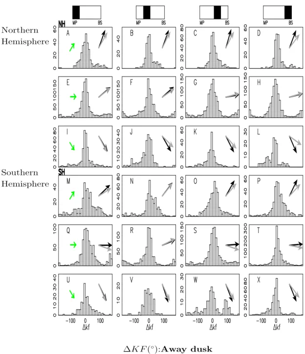
∆KF (

◦

):Away dusk

Northern

Hemisphere

Southern

Hemisphere

Fig. 5. 1_KF (in degrees) for the dusk dayside magnetosheath during intervals of away Parker spiral IMF: 1_KF represents the deviation of the observed magnetosheath magnetic field clock angle from that predicted by the KF model. The layout is the same as for Fig. 4.

binned in an identical way to the previous section in which we average over the entire magnetosheath thickness and plot the magnetosheath and KF model magnetic field directions at each longitude and latitude. Instead here we investigate the statistical presence of a rotation in at different regions of the magnetosheath which progress from the magnetopause to the bow shock boundary.

Each panel in Figs. 4–7 contains a histogram in which the magnetosheath magnetic field data are binned according to their clock angle deviation (in degrees) from the KF model prediction. Each panel thus represents the range of observed

clock angle deviation from the KF model prediction, for a given range of magnetosheath thickness located between the bow shock and magnetopause boundaries, and under a partic-ular configuration of the upstream IMF direction. The mean clock angles of the KF model prediction (black vector) and the magnetosheath magnetic field (grey vector) are indicated in the top left hand corner of each panel.

The statistical moments, mean µ (and standard error of mean, σM), standard deviation δ and kurtosis µ4of the

dis-tribution, are used in the analysis to allow a quantitative as-sessment of the following features; the mean rotation of the

(10)

∆KF (

◦

):Toward dawn

Northern

Hemisphere

Southern

Hemisphere

Fig. 6. 1_KF (in degrees) for the dawn dayside magnetosheath during intervals of toward Parker spiral IMF: 1_KF represents the deviation of the observed magnetosheath magnetic field clock angle from that predicted by the KF model. The layout is the same as for Fig. 4.

magnetosheath magnetic field direction from the KF model magnetic field direction and its statistical significance, the standard deviation of this mean, and the kurtosis (“peaked-ness”) of the distributions. In the following section we use a moments description for each distribution, examined in the context of the magnetosheath sector and IMF condition rep-resented by a particular histogram. Table 1 gives the values

of the mean shift µ, standard deviation δ and kurtosis, µ4

which correspond to each of the histograms, A-X in Figs. 4 and 5 (i.e. away Parker IMF). Table 2 gives the corresponding

statistical moments for the histograms A–X of Figs. 6 and 7 (toward Parker IMF).

3.3.1 Rotation under southward IMF

When the upstream IMF is directed in an away Parker di-rection and IMF clock angle is southward (135◦<θ <180◦) (Panels I–L (NH), U–X (SH) of Figs. 4 and 5), the magne-tosheath magnetic field clock angle generally peaks at values which are shifted from 0◦. This implies a general shift of the the magnetosheath magnetic field clock angle from the KF

(11)

∆KF (

◦

):Toward dusk

Northern

Hemisphere

Southern

Hemisphere

Fig. 7. 1_KF(in degrees) for the dusk dayside magnetosheath during intervals of toward Parker spiral IMF: 1_KF represents the deviation of the observed magnetosheath magnetic field clock angle from that predicted by the KF model. The layout is the same as for Fig. 4.

static magnetosheath field model. The shift is quantified by the mean, µ in Table 1. The standard error mean, σmis small

with respect to the mean and this mean shift is therefore sta-tistically significant. The majority of the distributions have a peakedness which exceeds that of a normally distributed data set (kurtosis, µ4, for a normally distributed data set is

3). The standard deviation, δ (see also Table 1) reflects the contribution of the smaller number of magnetosheath field data points within each distribution which show larger devi-ations from the KF model. Several distributions, which oc-cur in the Northern Hemisphere at dawn and for southward

IMF exhibit a broader, less well peaked distribution of mag-netosheath field clock angle than the majority (see values of kurtosis, µ4and standard deviation, δ for panels I, J and K

in Table 1:Dawn). Despite the large spread observed in some of the distributions, the mean magnetosheath magnetic field clock angle (grey vector) is rotated anti-clockwise from the KF model predicted clock angle (black vector) in 13 of the 16 panels representing cross-sections of the magnetosheath at both dawn and dusk during periods of away Parker spiral and southward IMF orientation.

(12)

Table 1. Statistical moments of the distributions shown in Figs. 4 and 5: away Parker IMF. Dawn Dusk µ σM δ µ4 µ σM δ µ4 A 22.03 2.0 39.12 4.82 11.88 2.68 47.85 4.52 B 12.04 2.26 45.37 8.56 8.39 2.6 38.21 4.54 C 10.27 1.7 36.45 10.18 13.68 1.9 37.33 5.99 D 1.92 1.64 43.02 7.64 18.9 2.12 32.92 5.81 E 3.28 2.01 58.56 3.99 1.94 2.09 70.6 4.19 F –10.35 1.78 56.95 4.68 5.29 2.05 68.82 4.36 G –12.75 1.57 51.95 5.38 –3.17 1.08 35.98 6.56 H –15.99 1.49 49.96 4.58 –1.72 1.42 45.52 7.75 I –22.65 5.0 68.05 2.7 3.14 2.6 50.93 5.33 J –10.74 6.81 83.17 2.73 –15.83 3.26 52.07 4.9 K –15.35 8.29 98.13 2.23 –15.16 3.02 46.23 5.05 L –29.38 4.83 71.22 3.22 –31.46 3.27 38.9 3.15 M 18.26 3.754 67.2 3.33 10.28 3.46 68.16 3.42 N 14.64 5.78 85.21 2.25 1.66 2.89 59.09 4.36 O 10.38 4.6 78.45 2.5 11.91 2.6 52.49 4.61 P 8.55 1.62 48.85 4.95 18.57 2.8 56.32 6.01 Q 14.76 3.47 77.816 2.94 13.67 1.8 52.63 6.61 R –16.15 2.88 73.39 3.9 –2.83 1.94 55.45 6.69 S 1.76 2.73 73.29 3.68 16.08 1.53 52.45 5.23 T 12.2 2.2 74.48 3.83 10.7 1.22 45.37 7.16 U 8.25 6.7 76.82 3.16 2.8 3.13 40.98 4.84 V –2.07 2.59 32.65 4.23 –8.32 7.113 75.9 2.96 W –8.03 3.74 53.63 4.54 –9.3 4.48 60.42 4.57 X –6.9 5.1 56.46 3.88 –16.78 1.96 38.31 5.03

Table 2. Statistical moments of the distributions shown in Figs. 6 and 7: toward Parker IMF.

Dawn Dusk µ σM δ µ4 µ σM δ µ4 A 24.6 6.6 81.59 2.41 -13.438 3.5 52.41 3.14 B 2.514 3.5 64.5 3.33 –0.58 2.7 43.67 6.94 C 14.98 6.2 75.11 3.38 –13.9 2.08 43.31 5.88 D 2.38 4.53 72.35 3.44 –9.38 1.7 30.04 10.06 E –0.99 5.65 85.38 2.55 1.94 1.32 52.09 5.87 F –0.15 5.0 71.82 3.8 2.14 1.43 53.76 7.42 G –8.2 2.3 64.24 3.67 1.72 0.93 37.26 11.61 H 6.13 2.53 73.8 3.35 0.03 0.68 26.23 10.75 I 19.11 1.44 43.03 5.1 9.25 2.13 42.2 7.24 J 23.18 1.45 50.57 4.56 8.8 2.02 39.76 5.03 K 9.94 2.97 52.65 3.58 12.38 1.92 37.71 9.06 L –29.38 2.73 52.025 6.04 13.3 2.03 34.79 6.5 M 6.37 1.81 23.7 14.7 –18.07 6.15 81.33 2.96 N 5.61 3.38 58.78 4.09 5.09 3.55 57.42 5.58 O –19.49 2.43 60.09 4.16 –0.06 2.35 44.95 4.29 P 1.19 7.95 80.27 3.6 –10.04 1.7 33.37 4.41 Q –4.73 4.04 64.92 4.13 2.91 2.25 69.59 4.15 R 6.13 4.19 71.43 4.33 4.92 1.59 53.49 5.75 S –1.3 2.59 65.7 4.57 3.95 1.48 56.66 6.43 T 10.28 1.98 54.75 5.74 8.99 1.21 46.1 9.24 U 4.11 2.17 58.07 3.51 –22.33 3.73 57.28 3.56 V 21.79 1.48 47.0 3.26 2.63 3.28 55.84 5.09 W 17.56 4.03 68.16 2.83 16.31 3.55 53.23 6.6 X 13.96 1.68 79.64 2.74 13.528 2.58 47.17 6.9

(13)

Table 3. Preferred clock angle rotation of magnetosheath magnetic field vector at dawn.

Toward Parker (no. of cases/8) Away Parker (no. of cases/8)

Northward IMF no preferred direction Clockwise (8/8)

Southward IMF Clockwise (8/8) Anti-Clockwise (6/8)

Table 4. Preferred clock angle rotation of magnetosheath magnetic field vector at dusk.

Toward Parker (no. of cases/8) Away Parker (no. of cases/8)

Northward IMF Anti-clockwise (6/8) Clockwise (8/8)

Southward IMF Clockwise (7/8) Anti-Clockwise (6/8)

Figures 6 and 7 show the distribution of the observed clock angle from model values for a toward directed Parker spi-ral, for dawn and dusk parts of the dayside magnetosheath respectively. In the case of toward oriented Parker IMF, the mean clock angle of the observed distributed deviations (grey vector) is rotated clockwise from the KF model predicted clock angle (black vector) in 14 of the 16 panels representing cross-sections of the magnetosheath at dawn and dusk under southward IMF.

3.3.2 Rotation under northward IMF

Under northward IMF (Panels A–D (Northern Hemisphere) and M–P (Southern Hemisphere)), the observed rotation of the mean clock angle from the KF model prediction is clock-wise for an away Parker spiral and generally anti-clockclock-wise for a toward Parker spiral. However under northward IMF at dawn, for toward Parker spiral, no clear preference is ob-served (see panels A, B, C, D, N, and O in Fig. 6 and 4.

As in the preceeding section, the analysis of the equatorial IMF data includes both northward and southward IMF within

45◦of the equatorial plane and therefore removes some of

the Bzeffect. We have excluded the possibility of observing

a Byinduced rotation in Sect. 3.2. The remaining rotation is

therefore likely to be due to the presence of the residual bias of either northward or southward cases contained within the averages representing equatorial IMF.

The preferred rotation directions of the magnetosheath magnetic field for northwards/ southwards and toward/away IMF (and the number of cases for which the preferred rota-tion is observed) are summarised Tables 3 and 4. The extent of the rotations, µ is typically >5◦and <30◦although these are associated with a significant standard deviation, δ (see Tables 1 and 2).

3.3.3 Rotation of the magnetic field by the bulk plasma

flow direction in the magnetosheath

In general, the preferred rotation of the magnetosheath mag-netic field under northward and southward IMF is consistent

with an interpretation which considers the dominant direc-tion for bulk plasma flow in the magnetosheath. The rotadirec-tion is absent from the KF static magnetic field model since it does not incorporate field-flow effects. Figure 8 shows the 2-D projection of the solar wind normalised velocity magni-tude in GSM latimagni-tude and longimagni-tude averaged over the mag-netosheath survey region taken from Longmore et al. (2005). Due to the orbital bias present in the surveyed region, data surveyed at low latitudes lies close to the bow shock region; data at higher latitudes is biased toward the magnetopause boundary. The flow is greatest at the flank regions of the magnetosheath. In Longmore et al. (2005) we showed that this is a generalised flow behaviour in the magnetosheath which is independent of upstream IMF directions. In Fig. 9, the magnetic field (indicated by red vectors) is frozen to the plasma flow and the ends of the magnetic field lines become stretched and pulled in the direction of the accelerated bulk plasma flow at the flanks. The interaction is most evident when a strong northward or southward IMF component is present. These magnetic field lines have a component per-pendicular to the direction of fast dawn and dusk ward bulk plasma flow and therefore undergo the most significant ro-tation. The twist (black vectors), which tends to rotate the magnetic fields, is clockwise in the case of an IMF oriented along a northward away or southward toward direction (ex-amples A and B in Fig. 9) and counter-clockwise for IMF ori-ented along a southward away or northward toward direction (examples C and D in Fig. 9). In this way the bulk plasma flow acts on the magnetic field lines to produce twisting of the IMF.

4 Discussion

In this paper we highlight the role of the bulk flow on field line draping in the magnetosheath. This effect on the mag-netic field line draping extends beyond both the gas-dynamic and simple KF static magnetic field models which do not in-corporate field-flow forces in models of the magnetosheath magnetic field line draping.

(14)

GSM Lati tude GSM Longitude V / V sw

Fig. 8. 2-D projection of the solar wind normalised velocity magnitude and velocity components averaged over the magnetosheath survey region (GSM). Due to the orbital bias present in the surveyed region, data surveyed at low latitudes lies close to the bow shock region; data at higher latitudes is biased toward the magnetopause boundary. The flow is greatest at the flank regions of the magnetosheath.

In Sect. 3.1 we described the KF model and noted the ab-sence of a field-flow coupling interaction in its description. This is an established feature of the magneospheric-solar wind coupling interaction and exhibits an effect on the drap-ing pattern in our analysis. The drapdrap-ing survey shows that the KF model is not adequate for a prediction of the magne-tosheath clock angle, particularly under strongly northward and southward IMF conditions. In this study, we have iso-lated the effect of the bulk velocity flow direction on the draping pattern in the magnetosheath. No such observation has been reported to date for the behaviour of the flow at the dayside magnetosheath, although field-flow coupling effects are well established features of the MHD description of the magnetosheath plasma.

We find an almost consistent rotation of the magnetosheath clock angle relative to the KF model prediction. The only exception is observed in the dawn magnetosheath during a northward, toward IMF orientation. In this case little or no preferred sense of rotation is observed. The observed clock angle directions indicated in the panels in Figs. 4, 5, 6 and 7 show that the mean rotation of the observations from the statistical analysis is the same as that illustrated in the vector

maps illustrated in Fig. 3. The rotation of the magnetic field is consistent with an interpretation which considers the dom-inant direction for bulk plasma flow in the magnetosheath given in Sect. 3.3.3.

Kaymaz et al. (1992) likewise reported a rotation of the ob-served magnetic field in the magnetotail. The Kaymaz et al. (1992) analysis is conducted somewhat differently and the rotation is defined relative to the plane formed by the IMF and an aberrated x-axis. In the case of Kaymaz et al. (1992), a counter-clockwise rotation for away IMF and a clockwise rotation for toward IMF was found for both northward and southward IMF. The rotation was found to reach a maximum for moderately southward IMF. In this analysis, we define a rotation relative to the KF model predicted clock angle and observe an effect for northward and southward IMF. This is a unanimous counter-clockwise rotation for away IMF and a clockwise rotation for toward IMF which is due to the bulk plasma flow direction in the magnetosheath rather than merg-ing at the dayside magnetopause. Arguably, our case for a preferential rotation sense under northward IMF is weak-ened by the behaviour observed at dawn during toward IMF but even here the rotation appears to be ambiguous rather

(15)

Fig. 9. Rotation of the draping pattern by the plasma flow in the dayside magnetosheath: The magnetic field (indicated by red vectors) is frozen to the plasma flow and the ends of the magnetic field lines become stretched and pulled in the direction of the accelerated bulk plasma flow at the flanks. The interaction is most evident when a strong northward or southward IMF component is present since these magnetic field lines have a component perpendicular to the direction of fast dawn and dusk ward bulk plasma flow and therefore undergo the most significant rotation. The twist (black vectors), which tends to rotate the magnetic fields, is clockwise in the case of an IMF oriented along a northward away or southward toward direction (Examples A and B in figure 9) and counter-clockwise for IMF oriented along a southward away or northward toward direction (Examples C and D in figure 9). In this way the bulk plasma flow acts on the magnetic field lines to produce twisting of the IMF.

33

Fig. 9. Rotation of the draping pattern by the plasma flow in the dayside magnetosheath: the magnetic field (indicated by red vec-tors) is frozen to the plasma flow and the ends of the magnetic field lines become stretched and pulled in the direction of the accelerated bulk plasma flow at the flanks. The interaction is most evident when a strong northward or southward IMF component is present since these magnetic field lines have a component perpendicular to the direction of fast dawn and dusk ward bulk plasma flow and there-fore undergo the most significant rotation. The twist (black vectors), which tends to rotate the magnetic fields, is clockwise in the case of an IMF oriented along a northward away or southward toward direction (Examples A and B in Fig. 9) and counter-clockwise for IMF oriented along a southward away or northward toward direc-tion (Examples C and D in Fig. 9). In this way the bulk plasma flow acts on the magnetic field lines to produce twisting of the IMF.

than the reverse of the sense of rotation observed in the other cases. Whilst Kaymaz et al. (1992) finds a rotation which is strongest for IMF with an equatorial component and which is associated with dayside merging, we do not observe a similar effect in our data. Such an effect would predominate in a nar-row region close to the dayside magnetopause whereas our analysis is concerned with the averaged draping behaviour observed throughout the dayside magnetosheath, from up-stream of the magnetopause to the bow shock boundary.

We conclude therefore that there are two observed draping effects in operation on the IMF as it enters the region down-stream of the bow shock. Kaymaz et al. (1992) show that their observed rotation in the tail magnetosheath is consistent with strengthened merging under southward IMF and tilting of the dayside merging line due to equatorial IMF compo-nents. This explanation explains why the rotation observed in their study is greatest under moderately southwards IMF. We observe a rotation of the magnetosheath field in regions away from the magnetopause boundary which cannot be in-terpreted in terms of merging at the magnetopause but which can be explained by the tendency of the bulk flow in the mag-netosheath proper to strengthen away from sub-solar regions toward the dawn and dusk flanks of the magnetosheath. Both findings highlight the importance of incorporating dayside

reconnection and field-flow forces into the description of draping around Earth’s magnetosphere.

We note that the distributions in the magnetosheath exhibit a significant spread of magnetic field clock angle direction. In some cases, less ordered distributions under northward and southward IMF, close to the magnetopause boundary, might indicate a less regulated draping behaviour in that re-gion. Such an effect under northwards IMF is generally con-fined to the high latitude inner sectors of the magnetosheath. With the exception of dawn in the Southern Hemisphere, the magnetosheath cross-sections exhibit decreases in the kurto-sis values and increases in the standard deviation from the bow shock to the magnetopause boundary (see for example Tables 1 and 2, Dawn: A, B, C, D, Dusk A, B ,C, D, M, N, O, P). This may indicate a transition in the vicinity of the high latitude magnetopause boundary into a region in which the draping pattern is less well ordered. Under southwards IMF we observe that the distributions in panels I, J and K of Fig. 4 are also flattened and have low values of kurtosis and large standard deviation. There is however no consistent decrease of the kurtosis or increase of the standard devia-tion toward the high latitude magnetopause boundary which clearly links the spread of observed clock angle with prox-imity to the magnetopause boundary.

Furthermore, inaccuracies in the lagging procedure, dur-ing periods of strong upstream solar wind variability most likely contribute to the observed broadening. Indeed, solar wind discontinuities, which produce sharp transitions in the upstream magnetic field strength and direction, sometimes invoke uncertainties in our estimate of the time lag which links the magnetosheath measurements with the upstream measurements at ACE. This is because the estimated time lag is precise to within only ≈5 min and during periods of strong solar wind variability the magnetic field direction may fluctu-ate between northward and southward IMF within very short time scales. Such intervals are included in the data set and are likely to produce some erroneous clock angle variation therein. This will artificially broaden the spread of clock an-gle observed and increase the standard deviation. However the majority of the distributions are well ordered around a central value which implies that the large number of magne-tosheath crossings used in the survey appear to compensate for the additional statistical noise introduced by inclusion of these interval. We conclude that the inclusion of such inter-vals does not pose a significant problem to the emergence of the systematic rotations observed for the magnetic field di-rection. On the other hand, the broadening also hampers de-termination of an estimate for the typical amount of rotation observed. In Tables 1 and 2 we observe typical mean rota-tions (µ) under northward and southward IMF which range from 5◦−30◦but which are typically associated with large standard deviation (δ).

We emphasise the significance of this result to studies which rely on a determination for the magnetosheath clock angle based on knowledge of the upstream IMF clock an-gle. Assuming the IMF clock angle is roughly preserved in the magnetosheath or that it can be predicted by either

(16)

the gas-dynamic or static magnetic field model of Kobel and Fl¨uckiger (1994) model would justify use of upstream ob-servations of the IMF as a method to predict the magnetic shearing angle at the magnetopause boundary when in-situ measurements of the local magnetosheath vector are unavail-able. We conclude that, the effect of magnetosheath flow on the IMF not considered by these models, results in poor ac-curacy of such methods. MHD models which incorporate field-flow coupling should provide a more accurate way to model the magnetosheath and a comparison of global MHD results for the dayside magnetosheath with the Cluster obser-vations is proposed for future work.

Acknowledgements. This research is supported by a studentship

from the UK Particle Physics and Astronomy Research council and, in part, by NASA Grant NNG05GG26G. We thank the Cluster FGM team for the use of magnetic field data used in this study. We also acknowledge the Cluster PEACE and CIS teams for data used in a previous study which contributes to the scientific conclusion of this paper. Additional solar wind data was provided by the MAG instrument team and the ACE Science Center. We extend thanks to the referee for a critical evaluation of this paper. Parts of the data analysis were carried out with the Cluster Science Analysis System, QSAS (Queen Mary, University of London and Imperial college London). All these sources were a vital part of this work.

Topical Editor T. Pulkkinen thanks M. Palmroth and another referee for their help in evaluating this paper.

References

Balogh, A., Carr, C. M., Acu˜na, M. H., Dunlop, M. W., Beek, T. J., Brown, P., Fornac¸on, K.-H., Georgescu, E., Glassmeier, K.-H., Harris, J., Musmann, G., Oddy, T., and Schwingenschuh, K.: The Cluster Magnetic Field Investigation: overview of in-flight performance and initial results, Ann. Geophys., 19, 1207–1217, 2001,

SRef-ID: 1432-0576/ag/2001-19-1207.

Behannon, K. W. and Fairfield, D. H.: Spatial variations of the magnetosheath magnetic field, Planetary and Space Science, 17, 1803–1816, 1969.

Coleman, I. J.: A multi-spacecraft survey of magnetic field line draping in the dayside magnetosheath, Ann. Geophys., 23, 885– 900, 2005,

SRef-ID: 1432-0576/ag/2005-23-885.

Cooling, B. M. A., Owen, C. J., and Schwartz, S. J.:

Role of the magnetosheath flow in determining the mo-tion of open flux tubes, J. Geophys. Res., 18 763–18 776, doi:10.1029/2000JA000455, 2001.

Crooker, N. U., Luhmann, J. G., Russell, C. T., Smith, E. J., Spre-iter, J. R., and Stahara, S. S.: Magnetic field draping against the dayside magnetopause, J. Geophys. Res., 90, 3505–3510, 1985. Fairfield, D. H.: The Ordered Magnetic Field of the Magnetosheath,

J. Geophys. Res., 72, 5865–5877, 1967.

Fedder, J. A. and Lyon, J. G.: The Earth’s magnetosphere is 165 RE

long: Self-consistent currents, convection, magnetospheric struc-ture, and processes for northward interplanetary magnetic field, J. Geophys. Res.h, 100, 3623–3635, 1995.

Fedder, J. A., Lyon, J. G., Slinker, S. P., and Mobarry, C. M.: Topo-logical structure of the magnetotail as a function of interplane-tary magnetic field direction, J. Geophys. Res., 100, 3613–3621, 1995.

Johnstone, A. D., Alsop, C., Burge, S., Carter, P. J., Coates, A. J., Coker, A. J., Fazakerley, A. N., Grande, M., Gowen, R. A., Gur-giolo, C., Hancock, B. K., Narheim, B., Preece, A., Sheather, P. H., Winningham, J. D., and Woodliffe, R. D.: Peace: a Plasma Electron and Current Experiment, Space Sci. R., 79, 351–398, 1997.

Kaymaz, Z.: IMP 8 magnetosheath field comparisons with models, Ann. Geophys., 16, 376–387, 1998,

SRef-ID: 1432-0576/ag/1998-16-376.

Kaymaz, Z., Siscoe, G., and Luhmann, J. G.: IMF draping around the geotail - IMP 8 observations, Geophys. Res. Lett., 19, 829– 832, 1992.

Kaymaz, Z., Siscoe, G., Luhmann, J. G., Fedder, J. A., and Lyon, J. G.: Interplanetary magnetic field control of magnetotail field: IMP 8 data and MHD model compared, J. Geophys. Res., 100, 17 163–17 172, 1995.

Kobel, E. and Fl¨uckiger, E. O.: A model of the steady state mag-netic field in the magnetosheath, J. Geophys. Res., 99, 23 617– 23 622, 1994.

Longmore, M., Schwartz, S. J., Geach, J., Cooling, B. A., Dan-douras, I., Lucek, E. A., and Fazakerley, A. N.: Dawn-dusk asymmetries and sub-Alfv´enic flow in the high and low latitude magnetosheath, Ann. Geophys., 23, 3351–3364, 2005,

SRef-ID: 1432-0576/ag/2005-23-3351.

Mobarry, C. M., Fedder, J. A., and Lyon, J. G.: Equatorial plasma convection from global simulations of the Earth’s magneto-sphere, J. Geophys. Res., 101, 7859–7874, 1996.

Paschmann, G., Baumjohann, W., Sckopke, N., Papamastorakis, I., and Carlson, C. W.: The magnetopause for large magnetic shear – AMPTE/IRM observations, J. Geophys. Res., 91, 11 099– 11 115, 1986.

Paschmann, G., Baumjohann, W., Sckopke, N., Phan, T.-D., and Luehr, H.: Structure of the dayside magnetopause for low mag-netic shear, J. Geophys. Res., 98, 13 409–13 423, 1993. Peredo, M., Slavin, J. A., Mazur, E., and Curtis, S. A.:

Three-dimensional position and shape of the bow shock and their vari-ation with Alfvenic, sonic and magnetosonic Mach numbers and interplanetary magnetic field orientation, J. Geophys. Res., 100, 7907–7916, 1995.

Rème, H., Aoustin, C., Bosqued, J. M., Dandouras, I., Lavraud, B., Sauvaud, J. A., Barthe, A., Bouyssou, J., Camus, T., Coeur-Joly, O., Cros, A., Cuvilo, J., Ducay, F., Garbarowitz, Y., Medale, J. L., Penou, E., Perrier, H., Romefort, D., Rouzaud, J., Vallat, C., Alcaydé, D., Jacquey, C., Mazelle, C., D’Uston, C., Möbius, E., Kistler, L. M., Crocker, K., Granoff, M., Mouikis, C., Popecki, M., Vosbury, M., Klecker, B., Hovestadt, D., Kucharek, H., Kuenneth, E., Paschmann, G., Scholer, M., Sckopke, N., Sei-denschwang, E., Carlson, C. W., Curtis, D. W., Ingraham, C., Lin, R. P., McFadden, J. P., Parks, G. K., Phan, T., Formisano, V., Amata, E., Bavassano-Cattaneo, M. B., Baldetti, P., Bruno, R., Chionchio, G., di Lellis, A., Marcucci, M. F., Pallocchia, G., Korth, A., Daly, P. W., Graeve, B., Rosenbauer, H., Va-syliunas, V., McCarthy, M., Wilber, M., Eliasson, L., Lundin, R., Olsen, S., Shelley, E. G., Fuselier, S., Ghielmetti, A. G., Lennartsson, W., Escoubet, C. P., Balsiger, H., Friedel, R., Cao, J.-B., Kovrazhkin, R. A., Papamastorakis, I., Pellat, R., Scudder, J., and Sonnerup, B.: First multispacecraft ion measurements in and near the Earth’s magnetosphere with the identical Cluster ion spectrometry (CIS) experiment, Ann. Geophys., 19, 1303–1354, 2001,

(17)

354 M. Longmore et al.: Rotation of the magnetic field in Earth’s magnetosheath Roelof, E. C. and Sibeck, D. G.: Magnetopause shape as a

bivari-ate function of interplanetary magnetic field Bzand solar wind

dynamic pressure, J. Geophys. Res., 98, 21 421–21 450, 1993. Sonnerup, B. U. O.: The reconnecting magnetosphere, in:

Magne-tospheric Physics, 23–33, 1974.

Spreiter, J. R. and Stahara, S. S.: A new predictive model for de-termining solar wind-terrestrial planet interactions, J. Geophys. Res., 85, 6769–6777, 1980.

Spreiter, J. R., Summers, A. L., and Alksne, A. Y.: Hydromagnetic flow around the magnetosphere, Planetary and Space Science, 14, 223–253, 1966.