Business cycle, reallocation of labor and asset prices

Business Cycle, Reallocation of Labor and Asset

Prices

by

Anton Petukhov

M.S., Moscow Institute of Physics and Technology (2013)

M.A., New Economic School (2013)

Submitted to the Sloan School of Management

in partial fulfillment of the requirements for the degree of

Master of Science in Management Research

at the

MASSACHUSETTS INSTITUTE OF TECHNOLOGY

September 2016

@

Massachusetts Institute of Technology 2016. All rights reserved.

Signature redacted

Author ...

..

of.

Management

loan School of Management

A

April 1, 2016

Certified by...Signature

redacted

Leonid Kogan

Nippon Telegraph and Telephone Professor

Thesis Supervisor

Signature redacted

Accepted by

MASSACHUSETTS INSTITUTE OF TECHNOLOGY

JUN 28 2016

I,

I

Catherine Tucker

Sloan Distinguished Professor of Management

Professor of Marketing

Chair MIT Sloan PhD Program

Business Cycle, Reallocation of Labor and Asset Prices

by

Anton Petukhov

Submitted to the Sloan School of Management on April 1, 2016, in partial fulfillment of the

requirements for the degree of Master of Science in Management Research

Abstract

Empirical literature on reallocation of resources during business cycles provides an evidence of increased reallocation of labor across firms during downturns. In this paper I build a theoretical model with search frictions in the labor market, that is consistent with this observation, and study implications of search and match frictions for the cross section of stock returns. In the model firms having more growth opportunities benefit from recessions due to more slack in the labor market which allows them to expand quicker and convert higher share of their growth opportunities into profitable projects. This feature generates a return spread between value and growth firms. In the model sorts of stocks based on different growth indicators yield patterns documented empirically in previous studies.

Thesis Supervisor: Leonid Kogan

Acknowledgments

I am extremely grateful to my thesis advisor Leonid Kogan. I thank him for

contin-uous encouragement, support and advising during preparation of this thesis.

I am in debt to my friends at Sloan and seminar participants at the MIT Sloan

Contents

1 Introduction 2 Empirical Motivation 3 The Model 4 Numerical Analysis 5 Conclusion A Tables B Figures 8 12 15 20 27 28 32

List of Figures

B-i Gross Job Reallocation in Manufacturing . . . . B-2 Log Unemployment Outflow Rate . . . .

32 32

List of Tables

A. 1 Book-to-Market Portfolios Returns and Unemployment in the Data 28

A.2 Baseline Calibration Parameters . . . . 29

A.3 Properties of Book-to-Market Sorted Portfolios . . . . 29

A.4 Properties of Earnings-to-Price Sorted Portfolios . . . . 30

A.5 Properties of Employment Growth Sorted Portfolios . . . . 30 A.6 Book-to-Market Portfolios Returns and Unemployment in the Model. 31 A.7 Properties of Simulated Portfolios with Constant Match Probability . 31

1. Introduction

In the seminal paper Davis & Haltiwanger (1992) propose several measures of job flows and describe their empirical properties for the manufacturing sector data in the

U.S. One of the striking patterns that they find in the data is that job destruction

rate is very volatile and highly countercyclical while job creation rate is much less volatile and almost acyclical. The measure of job reallocation proposed by Davis & Haltiwanger (1992) is highly countercyclical in the data. Literature on job reallocation grew very fast since then with additional empirical evidence both in favor and against the phenomenon and with theories attempting to explain it'.

In this paper I study potential implications of countercyclical reallocation for asset pricing. In particular I construct a theoretical model that features search and match frictions in the labor market along the lines of Mortensen & Pissarides (1994). The aggregate uncertainty in the economy is driven by the aggregate productivity shock. Firms in the economy differ by the composition of their assets: the amount of growth opportunities relative to the amount of assets in place. In the model bad times are times of high unemployment and hence hiring is much easier. This provides an opportunity for firms with higher growth potential to expand quicker. Thus during downturns labor is reallocated from mature to growing firms. This mechanism makes growth opportunities safer relative to assets in place giving rise to cross-sectional heterogeneity in stock returns. In accordance with previous empirical studies the

'Barlevy (2003), Blanchard & Diamond (1989, 1990), Burda & Wyplosz (1994), Caballero & Hammour (1994, 1996), Davis & Haltiwanger (1990, 1992), Davis et al. (2006, 2013), Davis et al.

(1998), Foote (1998), Foster et al. (2001), Foster et al. (2016), Fujita & Ramey (2009), Greenwood et al. (1996), Mortensen (1994), Mortensen & Pissarides (1994), Moscarini & Postel-Vinay (2009a,b), Roys (2014), Schuh et al. (1998), Shimer (2005, 2012) constitute an incomplete list of theoretical and empirical literature studying labor reallocation.

model generates heterogeneity in returns of portfolios formed based on different growth indicators such as earnings-to-price and book-to-market ratio (see e.g. Fama

& French 1992) or hiring rate (Belo et al., 2014). Empirically I find that

book-to-market sorted portfolios have different exposure to the shock to unemployment rate. In particular, loadings of returns on unemployment shock decrease monotonically from low book-to-market to high book-to-market portfolios. This result is in line with the intuition that growth firms can benefit from more slack in the labor market

in times of higher unemployment.

Theoretical literature attempting to explain cross-sectional heterogeneity in stock returns through firms' economic activity is large2. Here I find it most important to contrast my model with the theoretical models involving only one source of aggregate risk. Most of these models relate stock returns to firms' investment into physical capital decisions. In these models firms value is comprised from the value of assets in place and the value of growth opportunities. The difference between firms' risk may come from the difference in riskiness of their assets in place, the difference in riskiness of their growth opportunities and from difference of the share of growth opportunities versus assets in place in firms value. For example, in Berk et al. (1999)3 all firms have identical growth opportunities and controlling for market capitalization of the firm, high book-to-market signals higher riskiness of the assets in place giving rise to value premium. Similar mechanism is used in Gomes et al. (2003). In their model assets that have higher market value have lower conditional beta. Hence firms with higher book-to-market ratio have higher risk, which generates value premium. In both of these models value premium arises due to differences in risks between firms' assets in place and it is worth noting, that growth opportunities in these models are riskier than assets in place due to option-like payoff of the growth opportunities. Carlson et al. (2004) take a different approach. They introduce operational leverage and fixed adjustment costs into the model to make assets in place riskier than growth opportunities. In their model high book-to-market firms are firms with relatively

2_{Kogan & Papanikolaou (2012) contains a recent survey of the literature.}

3_{Apart from aggregate productivity shock the model of Berk et al. (1999) features also shocks to} the risk-free rate.

less growth options in their value which makes these firms riskier giving rise to value premium. Zhang (2005) utilizes similar mechanism but puts more accent on asymmetric adjustment costs and countercyclical risk premia. In this paper, as in Carlson et al. (2004) and Zhang (2005) heterogeneity in returns arises due to difference in risk between growth opportunities and assets in place, however this heterogeneity follows from a different mechanism. In my model due to procyclical cashflows the value of assets in place is procyclical as well. Value of growth opportunities, in contrast, is countercyclical. Booms are associated with low unemployment and tight labor market, whereas in downturns unemployment is high and labor market is loose. This generates countercyclical probability of growth opportunities turning into profitable assets in place and hence countercyclical variation in the value of growth opportunities.

This paper fits into the growing literature that studies the connection of the labor market with stock returns4. Danthine & Donaldson (2002) observe that smoother than aggregate productivity wage payments can generate operating leverage giving rise to equity premium and excess volatility. Gourio (2007) and Favilukis & Lin

(2015) argue that the same mechanism can explain heterogeneity in the cross-section

of stock returns. Merz & Yashiv (2007) introduce labor and capital adjustment costs into firm's profit maximization problem and study jointly investment, hiring decisions and stock returns in the cross-section. Belo et al. (2014) and Belo et al. (2015) find empirically that higher hiring rates predict lower stock returns in cross-section. They develop a theory involving adjustment costs shock that reproduces the results of their empirical study. As will be shown in Section 4, the model with single aggregate productivity shock proposed in this paper is capable to generate this predictability. Eisfeldt & Papanikolaou (2013) empirically find that higher organizational capital predicts lower stock returns and associate this finding with outside options of firms' key employees. Current work is most closely related to several papers that explicitly

4

An incomplete list of this literature includes Belo et al. (2014), Belo et al. (2015), Danthine & Donaldson (2002), Donangelo (2014), Eisfeldt & Papanikolaou (2013), Favilukis & Lin (2015), Gourio (2007), Merz & Yashiv (2007), Moscarini & Postel-Vinay (2010), Petrosky-Nadeau et al.

introduce labor market search frictions to study the connection between labor mar-ket dynamics and stock returns. Moscarini & Postel-Vinay (2010) introduce labor search frictions to connect cyclical hiring behaviour of large and small employers with profitability. Petrosky-Nadeau et al. (2013) study the effect of labor market search frictions on the aggregate stock market. In their model search frictions amplify aggregate shocks and generate disaster risks with properties similar to those observed in the data. From the modeling prospective my paper is closest to Simutin et al. (2014). Simutin et al. (2014) find that after controlling for conventional risk-factors firms with higher loadings on labor market tightness have lower future returns. To explain the observed pattern they construct a model with search frictions and shocks to matching technology bearing time-varying price of risk.

The rest of the paper is organized as follows. Section 2 reviews key stylized facts and empirical results that motivate this study. Section 3 presents the model. Section 4 contains calibration strategy and numerical results. Section 5 concludes.

2. Empirical Motivation

Davis & Haltiwanger (1992) define gross job reallocation as a sum of job destruction and job creation within a period of time, where job destruction is the absolute value of the total change of the number of employees in all shrinking establishments and

job creation is the absolute value of the total change of the number of employees

in all expanding establishments. On Figure B-1 I plot gross job reallocation in the manufacturing sector as a percentage of the total employment in the sector. The data comes from Davis et al. (2006) and BLS Business Employment Dynamics (see notes to Figure B-1 for details)1_{. One of the striking features of this plot is that gross} job reallocation spikes in recessions. This pattern is driven by sharp increases in job

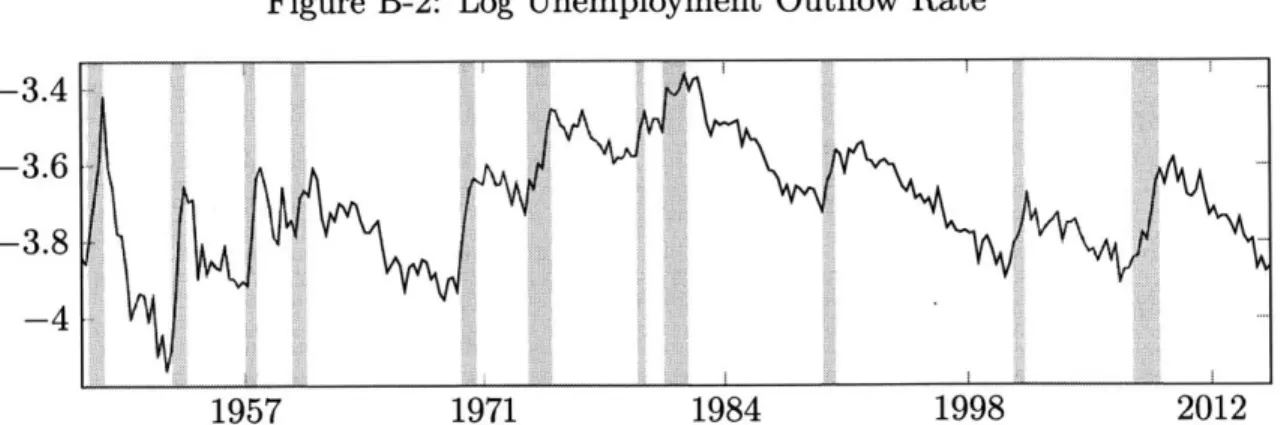
destruction rates and much less pronounced decreases in job creation during economic downturns. On Figure B-2 I present the logarithm of unemployment outflow as a share of labor force. This series is constructed using the job finding rate series constructed

by Shimer (2012) and data on unemployment-to-employment worker flows from the

Bureau of Labor Statistics (BLS). A remarkable pattern observed on this figure is that unemployment-to-employment flows tend to increase sharply during recessions2_.

These two patterns suggest that recessions are periods of increased turnover of workers through the unemployment pool and are periods of increased pace of hiring from the unemployment pool. Abundance of workers in the unemployment pool makes it easier for expanding firms to hire more people and find better matches for available

1I present job reallocation for the manufacturing sector only due to data availability. Existing series of job reallocation in the whole private sector are available from 1990 only.

2

Employment-to-unemployment worker flows increase during recessions too and this increase typically leads the increase of unemployment-to-employment flows, see e.g. Blanchard & Diamond (1990).

positions. Hence increased worker reallocation during recessions can be beneficial for these firms.

Vast empirical asset pricing literature documents that firms having more growth opportunities (as measured by different observable variables such as book-to-market equity ratio) have lower average stock returns. The evidence presented in the previous paragraph suggests that increased reallocation observed during economic downturns can act as a hedge for the "growth" firms, that get access to large pool of unemployed people and a big pool of talent with lack of employment opportunities. To test if fluctuations in reallocation have any relation to the cross-section of stock returns I run regressions of book-to-market sorted portfolios quarterly returns against changes in unemployment rate during the same period. I consider two specifications, with and without market excess return as a control variable:

R' - Rf =a + -y AUt + et, (2.1)

R' - Rf =a + ( R - Rf) + yAUt + Et ,(2.2)

here R' is a return on portfolio i in quarter t, Rf is the risk-free rate, R1 is market return and A Ut is the change in unemployment rate from quarter t - 1 to t. In this analysis I use five value-weighted book-to-market sorted portfolios published

by professor Kenneth R. French on his website and unemployment rate from BLS.

Data sample starts in 1948Q2 and ends in 2014Q4. Panel A of Table A.1 reports the estimates of -y in specification (2.1) for the five book-to-market sorted portfolios and 5 - 1 long/short portfolio. All five estimates for long portfolios are negative

reflecting intuition that times of higher unemployment are also times of lower stock market valuations. More interesting, the estimates decrease monotonically from low book-to-market to high book-to-market portfolio. Panel B reports results of the regression controlling for market excess returns. In this specification the estimates of -y are positive for low market portfolios and negative for high book-to-market portfolios. On top of that 5 - 1 spread loading on unemployment change is both statistically and economically significant: one percentage point change in

unemployment rate on average corresponds to 2% spread in realized returns. One can not give a causal interpretation to the results of these regressions. However, the results go in line with the hypothesis that more slack in the labor market can be beneficial for "growth" firms.

The evidence on countercyclical reallocation of labor and monotone loadings of book-to-market sorted portfolios on unemployment shocks motivate the theoretical model developed in the following section.

3. The Model

Time is discrete. The economy consists of a continuum of firms and a continuum of workers of measure 1. Every firm i in the beginning of period t is characterized

by the number of active projects N't and the number of not active projects N't.

The structure of the labor market is close to Mortensen & Pissarides (1994). An active project is matched with a worker, whereas a non-active project is not. Every period an active project generates profit zt, where zt is aggregate state dependent productivity which follows a first order Markov chain. I assume that profits are the same for every active project of every firm' and depend on the aggregate state only. Non-active projects do not generate cashflows. Thus a firm's i profit is iri t = zt N't.

Every period after production has happened an active project can disappear with exogenous state dependent probability Sa (zt), in which case the worker that was

matched with that project becomes unemployed. Non-active projects disappear with probability s"(zt). A non-active project can become active if matched with a worker. Matching happens with aggregate state dependent probability

g(ut, vt) q(ut,vt) = p .

Vt

Here by ut I denote an unemployment level in the economy and by vt an aggregate number of vacancies in the economy, p is a constant parameter of the matching

efficiency, g(ut, VOt) is constant returns to scale matching technology. More detailed definition of ut and Vt will be given below.

'This assumption is for simplicity and is not crucial for my results. The model can be extended by introducing idiosyncratic productivity shocks with similar results.

Entry and exit

Every period a firm exits the market with constant exogenous probability 6, in which case all of its projects disappear and employees become unemployed. To keep the mass of the firms constant every period a measure 6 of new firms enters the market.

A new firm owns no active projects, but owns a state dependent number A(zt) of non-active projects.

Timing

The timing within every period is the following: i) Aggregate productivity zt is revealed; ii) Production; iii) Share sn(zt) of non-active projects disappears, sa(zt)

share of active projects disappears (separated employees join labor force next period only), share 6_{(zt) of firms exit; iv) 6 mass of new firms enter the market with mean}

stock of non-active projects A(zt), entering firms participate in the labor market in the current period; v) Matching of non-active projects with unemployed workers happens (matched pairs become productive in the next period).

Matching and aggregation

To make non-active projects profitable firms post vacancies. A non-active project corresponds to one vacancy. Denoting by n n total number of non-active projects in the beginning of period t:

nn= N di, (3.1)

aggregate number of vacancies is determined by

vt = nn (1 - 6)(1 -- s"(zt)) + 6A(zt). (3.2)

This equation states that number of vacancies in period t equals number of non-active projects in the beginning of the period corrected for exit and destruction plus number of non-active projects of newly entering firms. Total labor force in the economy is

normalized to 1. So unemployment is given by:

ut = 1-n =1- Ni"t di, (3.3)

where n' - total number of projects in the economy that are active in the beginning of period t. Number of new matches arising in the economy is:

G(ut, vt) = p g(ut, vt). (3.4)

Formulation of this model allows aggregation using the law of large numbers. Dynamics of aggregate variables in the economy is completely described by equations

(3.2), (3.3), (3.4) and:

+1= n(1 - 6)(1 - Sa(Zt)) + G(ut, Vt),

n = (1 - )(1 - s,(zt)) + 6A(zt) - G(ut, vt) . (3.5)

Here the first equation describes the evolution of the number of active projects. Number of active projects in period t + 1 equals the number of active projects in period t corrected for exits and job destruction plus number of new matches in period t. The second equation describes the evolution of non-active projects. Taking into account equation (3.2), number of non-active projects in the beginning of period t +1 equals number of vacancies minus number of new matches in period t.

Stochastic discount factor

I postulate an exogenous stochastic discount factor dependent on realization of the

aggregate productivity shock zt. Stochastic discount between periods t and t + 1 is defined by:

M exp (-f - ^[zt+1 - EtZt+i]) (3.6)

Et [exp (--7[zt+1 - Etzt+i])]

This definition of the stochastic discount factor is close to Carlson et al. (2004). For positive y it has the feature that states corresponding to positive unexpected

changes in aggregate shock are discounted relatively more compared to the states corresponding to negative shocks. The difference from the stochastic discount factor used in Carlson et al. (2004) is the normalization term in the denominator of expres-sion (3.6). This normalization insures that risk-free rate is constant in every state of

the world and is equal to f.2

Pricing

All firms are financed by equity only, and I assume that dividend payments coincide

with firms' profits. I normalize number of shares of each firm to be 1. A firm i end of period t value,3 Vi,t, consists of value of its active projects, Vi' and value of non-active

"i' projects

Vi, t = Vi t + "V. (3.7)

Since all active projects in the economy have the same productivity and all non-active projects have the same probability of being matched with a worker Vi"' and Vi' can be written as

V =t "Ni+1 , (3.8)

where Vt and Vt are per unit values of active and non-active projects correspondingly. Values Vt aand Vtn are defined recursively by

Va = Et[Mt+l (zt+1 + (1- 6)(1 - sa(zt+l))V"+₁)], (3.9)

Vt = Et[Mt+1 ((1 - 6)(1 - s'(zt+₁))((ut+1, vt+i)V" 1 + (1 - q(ut+1,

vt+1))Vll))]-(3.10)

2

Constant risk-free rate is counterfactual. I utilize this specification of the SDF to highlight heterogeneity in the cross-section of stock returns generated by the mechanism studied in this paper. Time-varying risk-free rate introduces additional effects in the cross-section of expected returns.

3

Here and after I simplify notation and omit dependence of variables on aggregate state of the economy by introducing subscript t, e.g. Vi,t = V(zt, ni+1, nin).

Note that VI/ is a function of zt only and can be computed exactly using matrix inversion in case when zt follows a finite state Markov chain. Probability of a vacancy being matched in period t + 1, q(ut+1, Vt+1), depends on unemployment and number of vacancies in period t + 1. Using equations (3.2) and (3.3) these variables can be expressed through zt+1, na"1 and nn+1. Since values na+1 and n+1 are known in the

end of period t, value Vtn can be solved numerically on a grid of values for zt, ni+,

ntl+1

-Intuition

Equations (3.9) and (3.10) allow us to compare risks of assets in place and growth opportunities qualitatively. As it follows from equation (3.9) fluctuations of the value of active projects are driven by fluctuations of cashflows through aggregate

productivity zt+1, by fluctuations of destruction rate sa (zt+i) and by comovement of

aggregate shock with the stochastic discount factor. Cashflow is equal to zt+1 and hence procyclical, in my calibration sa(zt+l) is countercyclical, so both of these effects make V more volatile and procyclical, which increases the risk of assets in place.

From equation (3.10) it follows that fluctuations in the value of non-active projects are driven by fluctuations of V4, by fluctuations of sn(zt+i) and by fluctuations in the vacancy match probability q(ut+1, Vt+1). The value of an active project, Vta, is

procyclical. In my calibration destruction rate s'(zt+₁) is proportional to sa(zt+1)

and hence countercyclical. These two effects make the value of growth opportunities riskier. However, note that since cashflows from active projects are non-negative, it must be the case that Vta1 > V"1 in every state of the world. Since q(ut+i, vt+1) is increasing in unemployment and decreasing in vt, the term (q(ut+1, Vt+i)V 1 +

(1 - q(ut+1, t+i))Vn1) is less procyclical than Vl+ and can be even countercyclical

if q(ut+i, Vt+i) varies significantly with the business cycle. This observation makes growth opportunities safer than assets in place driving heterogeneity in returns across firms with different ratio of growth opportunities to assets in place. I confirm this intuition in the simulations of a calibrated version of the model in the next section.

4. Numerical Analysis

Calibration

The model is calibrated at the monthly frequency. Values of parameters chosen in my baseline calibration are summarized in Table A.2. I assume that logarithm of the aggregate shock zt follows AR(1) process:

In zt+i = p ln zt + o-zst+1, (4.1)

where Et+1 is iid with zero mean and unit variance. I discretize the process with nz = 3 aggregate states using the procedure described in Rouwenhorst (1995). I

set p = 0.92 to match average duration of the aggregate shock being in its lowest

state with the average duration of NBER recessions after 1927, which is about 13 months. I set cz = _{0.32 jointly with the sensitivity of the stochastic discount factor}

to aggregate shock parameter -y = 0.4 to match equity market premium 7.3%, and market volatility 17.3%. I set T = 0.002 to roughly match level of the risk-free rate in the economy, this value translates into annual rate of 2.4%. I follow Corhay et al.

(2015) and set monthly firm exit rate to S 0.01/3 which translates into 4% annual

exit rate.

Rate of active project destruction, sa, rate of non-active project destruction, so, and the number of non-active projects an entering firm owns depend on the aggregate productivity. In calibrating these variables I pursue three goals. First, I want to restrict the dependence of these parameters on aggregate state to avoid proliferation of parameters. _{Second, I want to generate dynamics of the labor market that is}

consistent with the dynamics observed in the data. Third, I am trying to connect these values to previous studies as much as possible. To achieve these goals I postulate the following functional dependencel

A(Zt) = Aozc,

s(Z) = s

s"(zt) = so z7'. (4.2) Here I assume r, > 0. Consistent with the business cycle stylized facts and common intuition, these functional forms and the sign constraint insure that number of new projects appearing in the economy is procyclical, project destruction rate is countercyclical and thus more jobs/active projects are destroyed in downturns and less in booms. Destruction rate of non-active projects has the same dependence on the aggregate shock as destruction rate of active projects to ensure that difference in risk between active and non-active projects is not driven by exogenously postulated destruction rate. Note that when aggregate shock takes its median value z = 1 we

have Sa(Zt) = sa, s"(zt) =s n. Using this observation I set sa = 0.02/3, which is close

to the average job destruction rate of 0.026/3 per month for firms in private sector with more than 1000 employees2. This value is also consistent with the common value for depreciation rate of capital used in the business cycles literature. I set sn = 0.0375/3,

this value translates into annual depreciation rate of non-active projects of 15%. Kung

(2015) uses this value for the depreciation rate of R&D stock. I pick values of AO and

, to match the mean value and standard deviation of monthly unemployment rate which are 5.8% and 1.7% correspondingly in my sample. Setting AO = 7.82 and

r = 0.59 achieves this goal.

Finally, I define values of parameters of the matching function. I use the constant

lFuture versions of the model will feature endogenous fluctuations of job destruction.

2_{Average job destruction rate for firms in private sector is computed for the sample from 1992 to}

return to scale matching function introduced by Ramey et al. (2000):

tuv

g(u, v) = _{(UV) + V,0)1/,o}uv (4.3)

where I set elasticity of the matching technology b = _{1.25. This value is used by}

Petrosky-Nadeau et al. (2013) and is very close to the value suggested by Ramey et al. (2000). I set the efficiency of the matching technology parameter P equal to

0.19. In the model of Ramey et al. (2000) this parameter is effectively set to 1. My

model features different assumptions about project arrival process and hence different dynamics of vacancies. This difference requires introduction of the matching efficiency parameter to obtain plausible values of the first two moments of unemployment and plausible mean value of worker flow from unemployment to employment (UE flow). In this calibration average monthly UE flow is 1% of the labor force. This value is slightly lower than 1.6%, the number obtained using data reported in Blanchard & Diamond (1990)3 study of the worker flows.

Portfolio Sorts

Empirical literature establishing connection between growth opportunities of firms and expected stock returns is very rich. Regardless of the measure associated with growth opportunities most of the studies reveal a similar pattern: higher growth opportunities forecast lower stock returns. Fama & French (1992) document that high book-to-market and earnings-to-price ratios positively forecast returns in cross-section; Titman et al. (2004) find that higher investment rate forecasts lower stock returns; Cooper et al. (2008) document that a firm's total asset growth negatively predicts stock returns; in a recent paper Belo et al. (2014) find that higher employment growth rates forecast lower stock returns. Even though signals used to construct portfolios in cited above papers are different, all of them are likely to represent some common feature between firms. Firms having low book-to-market ratio, high asset

3

Average stock of employed ppopulation in Blanchard & Diamond (1990) sample is 93.2 million, average stock of unemployed is 6.5 and average monthly UE flow is 1.6 million, this gives the UE transition rate of 1.6/(6.5 + 93.2) = 1.6%.

growth or employment growth are very likely to be the firms that have more growth opportunities.

In this section I evaluate the model's ability to generate negative relation between growth opportunities and expected returns. In the model a firm is represented by a collection of matched and unmatched projects. A project becomes active and production happens when it is matched with a worker. Hence number of the firm's active projects equals the number of workers employed by a firm. At the same time, one can view every project as unit of assets owned by a firm. In the model I abstract from investment spending, however if every matched project required some investment outlay then investment spending on projects the firm owns could be treated as book value of equity or physical capital, in this case ratio of book equity to market value of the firm would be proportional to the ratio of the number of active projects to the market value of the firm. Hence, in this model I relate the number of active projects-to-market equity ratio to the conventional book-to-market equity ratio.

To evaluate the performance of the model in its ability to generate cross sectional difference in expected returns I perform sorts of stocks in simulated data. I simulate 200 panels of 2500 firms of length 1500. For every simulated panel I discard the first

500 observations to let the model converge to its stationary regime. In all of the

experiments I focus on value-weighted portfolios. Equal-weighted portfolios yield the same qualitative results with slight differences in quantities.

In Table A.3 I present summary statistics of portfolios sorted based on book-to-market equity value. The first panel shows summary statistics for empirical portfolios. To compute these statistics I use the data downloaded from Kenneth R. French website. The sample period starts in January 1948 and ends in December 2014. The second panel reports mean values of summary statistics across 200 simulated panels. To make comparison of the simulated and empirical data fair I follow the timing conventions used by Fama & French (1992) when constructing portfolios in the simulated data. As can be seen the model generates a sizable spread between portfolios that is comparable to the data.

earnings-to-price ratio. Again empirical data comes from professor Kenneth R. French website. To construct earnings-to-price ratio in simulated data I calculate the sum of firm's monthly earnings in year y - 1 and divide it by stock price in the end of December of

year y - 1. The portfolios are formed in the end of June of year y. Again model

implied average returns have a substantial heterogeneity across portfolios, which roughly matches heterogeneity observed in the data. Fama & French (1992) argue that in the data heterogeneity in returns of stocks with different E/P ratio is captured

by book-to-market equity. In the model developed in this paper there is a very tight

relation between E/P and book-to-market ratio. Firms that have low book-to-market ratio are firms with a lot of growth opportunities and few active projects. Since only active projects generate earnings, low book-to-market firms have also low earnings-to-price ratios.

As was mentioned above, other indicators of growth, such as employment growth, investment-to-capital ratio, asset growth were found to predict lower stock returns in previous empirical studies. I check if similar patterns hold in the model. Since labor is the only production input in this model, I perform employment growth rate sort. I define yearly employment growth using the formula (N 1 - Nia )

/

(0.5(A+ 1

+N,)).

This definition of employment growth is used in Belo et al. (2014). I form portfolios in the end of June of year y using employment growth observed in year y - 1. The

results of this sort are presented in Table A.5. For comparison in this table I also present empirical portfolios sorted on hiring rate and constructed following Belo et al. (2014) methodology. Again in accordance with empirical studies faster growing firms yield lower stock returns. The intuition behind this result in the model is similar to the intuition behind sorts based on book-to-market and earnings-to-price. Faster growing firms are the firms that have bigger stock of non-active projects relative to active project. Hence, employment growth is essentially inversely related to the book-to-market and earnings-to-price ratios.

To further investigate performance of the model I run regressions (2.1) and (2.2) using model simulated data. Table A.6 reports results of these regressions. Consistent with the data, estimates of -y decrease with book-to-market quintiles in both

specifi-cations. One notable difference from empirical results is much higher magnitudes of the estimates of y. For example, 5-1 long/short portfolio loading on unemployment change is 3 times higher in the model simulated data relative to the real data. One of the reasons for this difference could be the "lagging" nature of unemployment. In the model both stock returns and unemployment respond to aggregate productivity shocks very fast. In reality unemployment reacts to changes in economic conditions much slower than stock returns.

Inspecting the mechanism

I the model active projects and non-active projects have different levels of risk.

Cross-sectional difference in returns is driven by the difference in composition of firms' sets of projects. Non-active projects are much safer than active projects because of the countercyclical fluctuations in unemployment. In bad times, when realization of the stochastic discount factor is high, unemployment tends to increase. Higher unemployment translates into higher probability for a non-active project to get matched with a worker, which increases the value of non-active projects. This mechanism makes non-active projects or growth opportunities much safer relative to active projects or assets in place. However, within the model non-active projects can potentially be safer than active projects even without frictions in the labor market.

In this section I conduct a comparative statics experiment to evaluate to which extent cross-sectional difference in average returns in the model is driven by the labor market

frictions.

For this purpose, I simulate the analog of the model abstracting from the labor market. More precisely, I solve the model and simulate panels of firms in the case when all of the parameters take the same values as presented in Table A.2, except that now I assume that probability for a non-active project to be matched with a worker is constant and is equal to the average value of this probability in the baseline calibration. As before I simulate 200 panels and do sorts based on book-to-market, earnings-to-price and employment growth rates. The results of these simulations are presented in Table A.7. One can see that heterogeneity in returns is still observed

among ten portfolios for all three sorts. However, the magnitude of the dispersion is much lower. For example, in the baseline version of the model 10-1 spread for book-to-market portfolios is 6.5%, in the version without matching frictions this spread is

1.8% only. This leads to the conclusion that labor market frictions are potentially an

important mechanism that can drive significant heterogeneity in the cross section of stock returns.

5. Conclusion

In this paper I study the hypothesis of how fluctuations in employment can generate heterogeneity in stock returns. I find empirical evidence that book-to-market sorted portfolios returns comove with unemployment in different ways: value stocks on average depreciate relatively more than growth stocks when unemployment goes up. This intuition and empirical findings motivate the theoretical model developed in this paper. The model links labor market search frictions with a firm risk of equity. Simulations of the model show that labor market frictions can be a powerful mechanism in generating heterogeneity in the cross-section of stock returns. In particular, it is shown than the mechanism is able to generate empirically documented patterns such as heterogeneity in returns on portfolios sorted based on earnings-to-price ratio, book-to-market equity, hiring rate. The main insight behind these results in the model is simple. Growth opportunities gain in value when matched with workers. Since probability of a non-active project to be matched with a worker is higher in recession, growth opportunities are less prone to lose value in recession, which makes them safer.

The model is consistent with aggregate patterns of labor market dynamics and delivers a rich set of predictions regarding hiring decision of firms with different characteristics.

A. Tables

Table A. 1: Book-to-Market Portfolios Returns and Unemployment in the Data Portfolio 1 2 3 4 5 5-1 A. 7 -0.20 -0.38 -1.13 -1.50 -2.30 -2.09 (1.44) (1.38) (1.46) (1.70) (1.58) (0.94) B. # 1.06 0.97 0.89 0.92 1.02 -0.04 (0.02) (0.03) (0.04) (0.05) (0.06) (0.08) - 0.60 0.36 -0.46 -0.80 -1.52 -2.12 (0.40) (0.23) (0.37) (0.61) (0.67) (0.93)

Notes: In Panel A I present results of the regressions of book-to-market equity sorted value weighted

portfolios returns on quarterly change in unemployment rate: R' - Rf = a + Y AUt + Et. Panel

B: results of the regressions of book-to-market equity sorted value weighted portfolios returns on quarterly change in unemployment rate and market excess return: Rt - Rf a + / (Re" - Rf) +

y A Ut + et. Newey-West autocorrealtion robust standard errors in parentheses. Data on portfolio returns is downloaded from Kenneth R. French web site: http: //mba. tuck. dartmouth. edu/pages/ f aculty/ken. french/data-library .html. Data sample is from 1948Q2 to 2014Q4.

Table A.2: Baseline Calibration Parameters

Parameter Symbol Value

Persistence of aggregate productivity p 0.92

Volatility of aggregate productivity O-z 0.32

Monthly risk-free interest rate f 0.002

Loading of the SDF on productivity shock l 0.4

Firm exit rate 6 0.01/3

Destruction rate of active projects in median state 0.02/3

Destruction rate of non-active projects in median state so0.0375/3

Number of projects owned by an entering firm in median state A0 7.82 Loading of destruction rates on aggregate productivity shock r 0.59

Elasticity of the matching technology 1.25

Coefficient of the matching efficiency A 0.19

Notes: These are parameter values used in the benchmark model. Detailed description of the choice of numerical values see in the text.

Table A.3: Properties of Book-to-Market Sorted Portfolios Portfolio 1 2 3 4 5 6 7 8 9 10 Data E[R - Rf] 6.93 7.62 7.68 7.95 8.67 8.85 8.63 10.19 10.66 12.09 / 1.07 1.00 0.98 0.98 0.90 0.93 0.90 0.92 0.96 1.09 0- 17.01 15.53 15.19 15.59 14.67 14.95 15.02 15.63 16.35 19.82 Model E[R - Rf] 4.34 7.49 9.09 9.95 10.42 10.65 10.78 10.80 10.84 10.84 / 0.65 1.02 1.21 1.32 1.37 1.40 1.41 1.42 1.42 1.42 0- 11.56 17.83 21.02 22.80 23.77 24.28 24.52 24.61 24.65 24.67

Notes: The table reports annualized mean excess return (%), market beta and annualized volatility

(%) of portfolios sorted based on book-to-market equity ratio, firms in postfolio 1 have the lowest book-to-market ratio. Data on portfolio returns is downloaded from Kenneth R. French web site: http: //mba. tuck. dartmouth. edu/pages/f aculty/ken. french/datajlibrary. html. Data sample is from January 1948 to December 2014.

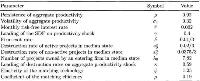
Table A.4: Properties of Earnings-to-Price Sorted Portfolios Portfolio 1 2 3 4 5 6 7 8 9 10 Data E[R - Rf] 6.29 5.77 7.21 7.04 7.75 9.22 9.86 10.73 11.48 12.51 #3 1.17 1.01 0.95 0.91 0.93 0.90 0.89 0.91 0.96 1.04 0- 18.95 15.82 15.18 14.66 14.96 14.87 14.72 15.42 16.38 17.89 Model E[R - Rf] 5.71 8.11 9.39 10.09 10.48 10.70 10.78 10.81 10.83 10.84 0.81 1.10 1.25 1.33 1.38 1.40 1.41 1.42 1.42 1.42 14.30 19.04 21.62 23.09 23.90 24.34 24.54 24.62 24.65 24.67 Notes: The table reports annualized mean excess return (%), market beta

(%) of portfolios sorted based on earnings-to-price ratio, firms in postfolio 1

and annualized volatility have the lowest earnings-to-price ratio. Data on portfolio returns is downloaded from Kenneth R. French web site: http: // mba. tuck. dartmouth. edu/pages/f aculty/ken. f rench/data-library .html. Data sample is from

July 1951 to December 2014.

Table A.5: Properties of Employment Growth Sorted Portfolios Portfolio 1 2 3 4 5 6 7 8 9 10 Data E[R - Rf] 7.58 7.38 5.75 6.97 4.64 6.29 5.56 5.20 6.07 4.38 ,3 1.00 0.90 0.85 0.89 0.91 0.96 1.00 1.09 1.12 1.15 0- 17.10 15.74 15.10 15.39 15.63 16.30 17.17 18.56 18.86 19.67 Model E[R - Rf] 10.83 10.83 10.81 10.79 10.69 10.49 10.10 9.41 8.14 5.73 /3 1.42 1.42 1.42 1.41 1.40 1.38 1.33 1.25 1.10 0.82 0- 24.68 24.65 24.62 24.54 24.35 23.91 23.11 21.65 19.10 14.35 Notes: The table reports annualized mean excess return (~ aktbt n ni~ie volatility (%) _{of simulated portfolios sorted based on employment growth defined as (Ni",t+1}

2

-Ngt)/(0.5(Nit2+Ngt)), firms in portfolio 1 have the lowest employment growth. Data on portfolio returns is constructed following methodology of Belo et al. (2014). Data sample is from July 1964 to December 2014.

Table A.6: Book-to-Market Portfolios Returns and Unemployment in the Model Portfolio 1 2 3 4 5 5-1 A. 7 -8.86 -13.48 -14.90 -15.28 -15.33 -6.47 (0.58) (0.86) (0.94) (0.97) (0.97) (0.46) B. / 0.57 0.87 0.95 0.97 0.98 0.40 (0.05) (0.07) (0.08) (0.08) (0.08) (0.04) ' -12.41 -18.83 -20.99 -21.57 -21.64 -9.23 (1.12) (1.68) (1.86) (1.91) (1.92) (0.93)

Notes: In Panel A I present results of the regressions of book-to-market equity sorted value weighted portfolios returns on quarterly change in unemployment rate: R - Rf a + y AUt + Et. Panel

B: results of the regressions of book-to-market equity sorted value weighted portfolios returns on quarterly change in unemployment rate and market excess return: R' - Rf = a + / (Re - Rf) +

-y AUt + Et.

Table A.7: Properties of Simulated Portfolios with Constant Match Probability Portfolio 1 2 3 4 5 6 7 8 9 10 Book-to-Market E[R - Rf] 9.04 10.06 10.49 10.67 10.77 10.78 10.82 10.83 10.81 10.81 # 0.91 1.02 1.06 1.08 1.09 1.10 1.10 1.10 1.10 1.10 0- 20.31 22.72 23.77 24.25 24.47 24.56 24.58 24.60 24.60 24.62 Earnings-to-Price E[R - Rf] 9.51 10.22 10.55 10.72 10.77 10.80 10.82 10.82 10.81 10.80

/

0.96 1.03 1.07 1.09 1.09 1.10 1.10 1.10 1.10 1.10 - 21.39 23.14 23.95 24.33 24.50 24.56 24.59 24.60 24.60 24.62 Hiring Rate E[R - Rf] 10.80 10.82 10.82 10.81 10.80 10.77 10.72 10.55 10.22 9.52

/3

1.10 1.10 1.10 1.10 1.10 1.09 1.09 1.07 1.03 0.96 0- 24.62 24.60 24.60 24.59 24.56 24.50 24.33 23.96 23.16 21.41 Notes: Each panel reports annualized mean excess return (%), market beta and annualized volatility

(%) of simulated portfolios sorted based on: book-to-market ratio, earnings-to-price ratio and employment growth defined as (Nit%_{1 2}- Ni)/(0.5(Nt+ 1 2 + N't)).

B. Figures

Figure B-1: Gross Job Reallocation in Manufacturing

16... . . . ... . . . I---16 -- ---14 12 10 8 6 1957 1971 1984 1998 2012

Notes: Gross job reallocation is defined as sum of job creation and job destruction. Numbers are percentages of employment. Source: 1947Q1 - 1992Q4 Davis et al. (2006), 1993Q1 - 2015Q1 BLS

Business Employment Dynamics.

Figure B-2: Log Unemployment Outflow Rate -3.4

-3.6 -3.8

-4

1957 1971 1984 1998 2012

Notes: Logarithm of unemployment outflow as share of labor force. Source: July 1948 - March 1990 constructed using job finding rate from Shimer (2012), April 1990 - Oct 2015 BLS; second series is shifted to obtain continuous graph.

Bibliography

Barlevy, G. (2003). Credit market frictions and the allocation of resources over the business cycle. Journal of Monetary Economics, 50(8), 1795-1818.

Belo, F., Lin, X., & Bazdresch, S. (2014). Labor hiring, investment, and stock return predictability in the cross section. Journal of Political Economy, 122(1), 129-177. Belo, F., Lin, X., & Li, J. (2015). Labor heterogeneity and asset prices: the

importance of skilled labor. Working paper.

Berk, J. B., Green, R. C., & Naik, V. (1999). Optimal investment, growth options, and security returns. The Journal of Finance, 54(5), 1553-1607.

Blanchard, 0. & Diamond, P. (1990). The cyclical behavior of the gross flows of us workers. Brookings Papers on Economic Activity, 21(2), 85-156.

Blanchard, 0. J. & Diamond, P. (1989). The Beveridge curve. Brookings Papers on

Economic Activity, 20(1), 1-76.

Burda, M. & Wyplosz, C. (1994). Gross worker and job flows in europe. European

economic review, 38(6), 1287-1315.

Caballero, R. J. & Hammour, M. L. (1994). The cleansing effect of recessions.

American Economic Review, 84(5), 1350-1368.

Caballero, R. J. & Hammour, M. L. (1996). On the timing and efficiency of creative destruction. The Quarterly Journal of Economics, 111(3), 805-52.

Carlson, M., Fisher, A., & Giammarino, R. (2004). Corporate investment and asset price dynamics: implications for the cross-section of returns. The Journal of Finance, 59(6), 2577-2603.

Cooper, M. J., Gulen, H., & Schill, M. J. (2008). Asset growth and the cross-section of stock returns. The Journal of Finance, 63(4), 1609-1651.

Corhay, A., Kung, H., & Schmid, L. (2015). Competition, markups and predictable returns. Working paper.

Danthine, J.-P. & Donaldson, J. B. (2002). Labour relations and asset returns. Review

Davis, S. J., Faberman, R. J., & Haltiwanger, J. C. (2006). The flow approach to labor markets: New data sources and micro-macro links. Journal of Economic

Perspectives, 20(3), 3-26.

Davis, S. J., Faberman, R. J., & Haltiwanger, J. C. (2013). The establishment-level behavior of vacancies and hiring. The Quarterly Journal of Economics, 128(2),

581-622.

Davis, S. J. & Haltiwanger, J. (1990). Gross job creation and destruction: Mi-croeconomic evidence and maMi-croeconomic implications. In NBER MaMi-croeconomics

Annual 1990, Volume 5 (pp. 123-186). MIT Press.

Davis, S. J. & Haltiwanger, J. (1992). Gross job creation, gross job destruction, and employment reallocation. The Quarterly Journal of Economics, 107(3), 819-863. Davis, S. J., Haltiwanger, J. C., & Schuh, S. (1998). Job creation and destruction.

The MIT Press.

Donangelo, A. (2014). Labor mobility: Implications for asset pricing. The Journal of

Finance, 69(3), 1321-1346.

Eisfeldt, A. L. & Papanikolaou, D. (2013). Organization capital and the cross-section of expected returns. The Journal of Finance, 68(4), 1365-1406.

Fama, E. F. & French, K. R. (1992). The cross-section of expected stock returns. The

Journal of Finance, 47(2), 427-465.

Favilukis, J. & Lin, X. (2015). Wage rigidity: A solution to several asset pricing puzzles. Review of Financial Studies, 29(1), 148-192.

Foote, C. L. (1998). Trend employment growth and the bunching of job creation and destruction. Quarterly Journal of Economics, 113(3), 809-834.

Foster, L., Grim, C., & Haltiwanger, J. (2016). Reallocation in the Great Recession: Cleansing or not? Journal of Labor Economics, 34(1).

Foster, L., Haltiwanger, J. C., & Krizan, C. J. (2001). Aggregate productivity growth: Lessons from microeconomic evidence. In New developments in productivity analysis

(pp. 303-372). University of Chicago Press.

Fujita, S. & Ramey, G. (2009). The cyclicality of separation and job finding rates.

International Economic Review, 50(2), 415-430.

Gomes, J., Kogan, L., & Zhang, L. (2003). Equilibrium cross section of returns.

Journal of Political Economy, 111(4).

Gourio, F. (2007). Labor leverage, firms&A2 heterogeneous sensitivities to the business cycle, and the cross-section of expected returns. Unpublished working paper, Boston University.

Greenwood, J., MacDonald, G. M., & Zhang, G.-J. (1996). The cyclical behavior of

job creation and job destruction: a sectoral model. Economic Theory, 7(1), 95-112.

Kogan, L. & Papanikolaou, D. (2012). Economic activity of firms and asset prices.

Annual Review of Financial Economics, 4(1), 361-384.

Kung, H. (2015). Macroeconomic linkages between monetary policy and the term structure of interest rates. Journal of Financial Economics, 115(1), 42-57.

Merz, M. & Yashiv, E. (2007). Labor and the market value of the firm. The American

Economic Review, 97(4), 1419-1431.

Mortensen, D. T. (1994). The cyclical behavior of job and worker flows. Journal of

Economic Dynamics and Control, 18(6), 1121-1142.

Mortensen, D. T. & Pissarides, C. A. (1994). Job creation and job destruction in the theory of unemployment. The Review of Economic Studies, 61(3), 397-415.

Moscarini, G. & Postel-Vinay, F. (2009a). Large employers are more cyclically sensitive. Technical report, National Bureau of Economic Research.

Moscarini, G. & Postel-Vinay, F. (2009b). The timing of labor market expansions: New facts and a new hypothesis. In NBER Macroeconomics Annual 2008, Volume

23 (pp. 1-51). University of Chicago Press.

Moscarini, G. & Postel-Vinay, F. (2010). Unemployment and small cap returns: The nexus. The American Economic Review, 100(2), 333-337.

Petrosky-Nadeau, N., Zhang, L., & Kuehn, L.-A. (2013). Endogenous disasters and asset prices. Charles A. Dice Center Working Paper.

Ramey, G., Haan, W. J. d., & Watson, J. (2000). Job destruction and propagation of shocks. American Economic Review, 90(3), 482-498.

Rouwenhorst, K. G. (1995). Asset pricing implications of equilibrium business cycle models. In T. Cooley (Ed.), Frontiers of Business Cycle Research. Princeton, NJ: Princeton University Press.

Roys, N. (2014). Persistence of shocks and the reallocation of labor. Working paper. Schuh, S., Triest, R. K., et al. (1998). Job reallocation and the business cycle: New

facts for an old debate. In Conference Series-Federal Reserve Bank of Boston, volume 42 (pp. 271-337).: Federal Reserve Bank of Boston.

Shimer, R. (2005). The cyclicality of hires, separations, and job-to-job transitions.

Review-Federal Reserve Bank OF Saint Louis, 87(4), 493.

Shimer, R. (2012). Reassessing the ins and outs of unemployment. Review of Economic Dynamics, 15(2), 127-148.

Simutin, M., Wang, J., & Kuehn, L. (2014). A labor capital asset pricing model.

Working paper.

Titman, S., Wei, K.-C., & Xie, F. (2004). Capital investments and stock returns.

Journal of financial and Quantitative Analysis, 39(04), 677-700.