Gene Regulatory Network Evolution Through Augmenting Topologies
Texte intégral
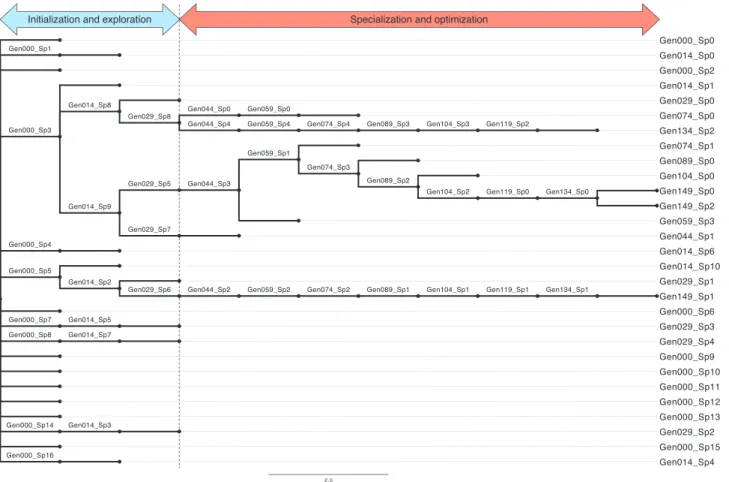
Figure


Documents relatifs
Therefore we have a décision method for the inclusion of pattern languages in only one of the four cases. Clearly, this does not imply that the other problems are undecidable.
Our findings showed that using a list of common entities and a simple, yet robust set of distributional similarity measures was enough to describe and assess the degree of
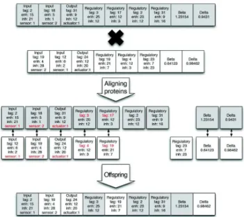
In a population of N organisms,having a mean number of genes of M and whose evolution is simulated.. T o ompute the anity of a protein with a given binding site, we align the
Informational masking mainly at the phonological level (Reverse – Noise), that is when the babble contained only partial phonetic information, activated the left primary
The resulting translated keys were used as queries and run against the target language data with Lemur retrieval system.. Date of publication and size are used to further
L’objet de notre essai a été d’étudier l’évolution du pH ruminal, sanguin et urinaire durant le développement d’une acidose latente provoquée sur moutons et lors de
Macroscopic scale: when stochastic fluctuations are neglected, the quantities of molecu- les are viewed as derivable functions of time, solution of a system of ODE’s, called
In other words, for each calculation, we have a unique difference matrix, allowing to compare result of variability for columns (technical coefficients) and for rows
