Assessing Calibration Uncertainty in Molecular Dating: The Assignment of Fossils to Alternative Calibration Points

ISSN: 1063-5157 print / 1076-836X online DO1:10.1080/10635150701491156

Assessing Calibration Uncertainty in Molecular Dating: The Assignment of Fossils

to Alternative Calibration Points

FRANK RUTSCHMANN,1 TORSTEN ERIKSSON,2 KAMARIAH ABU SALIM,3 AND ELENA CONTI1

1 _{Institute of Systematic Botany, University of Zurich, Zollikerstrasse 107, CH-8008 Zurich, Switzerland; E-mail: frank@plant.ch} 2_{Bergius Foundation, Royal Swedish Academy of Sciences, SE-104 05 Stockholm, Sweden}

3

Universiti Brunei Damssalam, Department of Biology, Jalan Tungku Link, Gadong BE 1410, Negara Brunei Darussalam

Abstract.—Although recent methodological advances have allowed the incorporation of rate variation in molecular dating

analyses, the calibration procedure, performed mainly through fossils, remains resistant to improvements. One source of uncertainty pertains to the assignment of fossils to specific nodes in a phylogeny, especially when alternative possibilities exist that can be equally justified on morphological grounds. Here we expand on a recently developed fossil cross-validation method to evaluate whether alternative nodal assignments of multiple fossils produce calibration sets that differ in their internal consistency. We use an enlarged Crypteroniaceae-centered phylogeny of Myrtales, six fossils, and 72 combinations of calibration points, termed calibration sets, to identify (i) the fossil assignments that produce the most internally consistent calibration sets and (ii) the mean ages, derived from these calibration sets, for the split of the Southeast Asian Crypteroni-aceae from their West Gondwanan sister clade (node X). We found that a correlation exists between s values, devised to measure the consistency among the calibration points of a calibration set (Near and Sanderson, 2004), and nodal distances among calibration points. By ranking all sets according to the percent deviation of s from the regression line with nodal distance, we identified the sets with the highest level of corrected calibration-set consistency. These sets generated lower standard deviations associated with the ages of node X than sets characterized by lower corrected consistency. The three calibration sets with the highest corrected consistencies produced mean age estimates for node X of 79.70, 79.14, and 78.15 My. These timeframes are most compatible with the hypothesis that the Crypteroniaceae stem lineage dispersed from Africa to the Deccan plate as it drifted northward during the Late Cretaceous. [Biogeography; calibration point; cross-validation; divergence times; fossil calibration; Myrtales; molecular dating; out-of-India.]

The use of DNA sequences to estimate the timing of evolutionary events is increasingly popular. Based on the central idea that the differences between the DNA sequences of two species are a function of the time since their evolutionary separation (Zuckerkandl and Pauling, 1965), molecular dating has been used as a method to investigate both patterns and processes of evolution (Magall6n, 2004; Renner, 2005; Rutschmann, 2006; Sanderson et al., 2004; Welch and Bromham, 2005).

However, significant methodological challenges affect the use of molecular dating approaches (Pulquerio and Nichols, 2007). Although recent studies have addressed the issue of variation among substitution rates (Aris-Brosou and Yang, 2002; Ho and Larson, 2006; Kishino et al., 2001; Penny, 2005; Rutschmann, 2006; Sanderson, 1997,2002; Thome et al., 1998; Yang, 2004), other difficul-ties persist, especially concerning the calibration proce-dure (Conti et al., 2004; Lee, 1999; Magallon, 2004; Reisz and Miiller, 2004). Calibration consists in the incorpora-tion of independent (nonmolecular) chronological infor-mation in a phylogeny to transform relative into absolute divergence times. This information can be based on ge-ological events (e.g., patterns of continental drift, origin of islands and mountain chains) and/or the paleonto-logical record (fossils). Geopaleonto-logical calibrations points are assigned to phylogenetic nodes based on the assump-tion that a geographic barrier caused phylogenetic diver-gence, thus generating the risk of circular reasoning, if the chronogram derived from the calibration is used to test biogeographical scenarios (Conti et al., 2004; Magall6n, 2004). Nevertheless, geological events can provide im-portant validation of dating estimates produced with

other types of calibration (e.g., Bell and Donoghue, 2005; Conti et al., 2002; Sytsma et al., 2004).

Although the fossil record is widely regarded as the best source of nonmolecular information about the ages of selected clades (Magall6n and Sanderson, 2001; Marshall, 1990b; Sanderson, 1998), several problems plague its use for calibration purposes, including (i) er-roneous fossil age estimates, (ii) the idiosyncrasies of fos-silization, (iii) the assignment of fossils to specific nodes in a phylogeny, and (iv) the number of fossils used for calibration. In this paper we focus primarily on the two latter aspects of fossil calibration, although all four prob-lems are interrelated.

Erroneous fossil age estimates may depend on mis-leading stratigraphic correlations or improper radiomet-ric dating (Conroy and van Tuinen, 2003) and the source of the error can only be addressed by improving the geo-logical dating procedures, whereas the effect of the error on molecular dating analyses can be partially addressed by the recently developed fossil cross-validation proce-dure (Near and Sanderson, 2004; see below).

The idiosyncrasies of the fossilization process may cause the failure of entire species to be preserved or discovered as fossils (Darwin, 1859). This lack of infor-mation makes it difficult or impossible to estimate the temporal gaps between the divergence of two lineages, the origin of a synapomorphy, and the discovery of that synapomorphy in the fossil record (see fig. 1 in Foote and Sepkoski, 1999; Magall6n, 2004; Springer, 1995). Fossils can thus provide only minimum ages for any lineage, a realization that is now incorporated in dating methods by treating the fossil ages assigned to calibration nodes as upper bounds, rather than fixed constraints (Sanderson 591

Dactylocjadus stenostachys Crypteronia paniculata Crypteronia bomeensis Crypteronia griffithii Crypteronia glabrifolia Axinandra zeylanica Axinandra coriacea Alzatea verticillata Rhynchocalyx lawsonioides 1 9 0 J j - Olinia radiata | U ~ Olinia ventosa • ' Olinia capensis I f Olinia emarginata I M ^ ~ Olinia vanguerioides Endonema retwides Endonema laterifiora Glischrocolla formosa Brachysiphon rupestris Stylapterus frupculosus Srylapterus ericoides ssp. pallidus — Brachysiphon fucatus Penaea acubfolia

Penaea cneorum ssp. gigantea Penaea cneorum ssp. ovata Penaea cneorum ssp. lanceolata

Penaea mucronata Penaea cneorum ssp. cneorum Penaea cneorum ssp. ruscifolia Brachysiphon micropnyllus Penaea dahlgrenii Stylapterus ericifolius Stylapterus micranthus Brachysiphon acutus Brachysiphon mundii Saltera sarcocolla Sonderothamnus petraeus Sonderothamnus speciosus Memecylon durum Memecylon edule • Ptemandra echinata Pternandra caerulescens

a

Melastoma beccarianum Melastomeae • Tibouchina urvilleana J Bertolonia marmorata Clidemia petiolaris Tococa guianensis Miconia donaeana Meriania macrophylla • Graffenrieda latirolia Macrocentrum cristatum Miconieae Merianieae Melaleuceae Eucalypteae Leptospermeae J Psiloxyloideae Myrtaceae s.s. Cuphea hyssopifolia* Crypteroniaceae Alzateaceae Rhynchocalycaceae Oliniaceae Penaeaceae Memecylaceae Melastomataceae Myrtaceae s.l. Vochysiaceae Onagraceae Lythraceae

0.1 substitutions per site Maximum Likelihood bootstrap support (10

3

reps.) Bayesian clade credibility

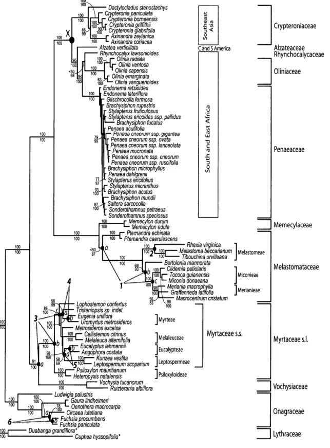
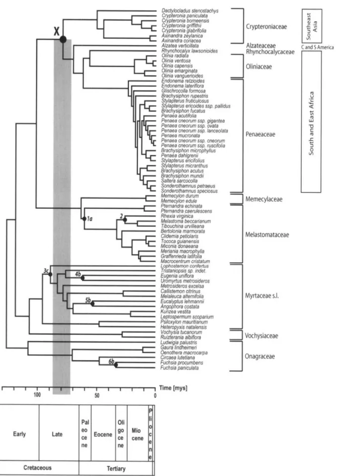
FIGURE 1. MrBayes majority-rule consensus tree with maximum likelihood branch lengths optimized in estbranches, based on the 5124-nucleotide data set. Maximum likelihood bootstrap support values and Bayesian clade credibility values are reported above and below the branches, respectively. General distribution ranges of the focus groups are reported to the right of the tree, as are the infrafamilial ranks relevant to fossil nodal assignments. Node X represents the phylogenetic split between the Southeast Asian Crypteroniaceae stem lineage and its African/South American sister clade. Alternative nodal assignments (a, b, or c) for the six fossils listed in Table 1 (numbers 1 to 6) are labeled on the tree. Outgroup taxa are indicated by an asterisk.

2003; Thorne and Kishino, 2002). Furthermore, recently developed methods attempt to estimate the gap between the time of first appearance of a synapomorphy in the fossil record and the time of divergence between two lin-eages by assuming that the size of the gap is inversely cor-related with the quality and density of the fossil record within a given stratigraphic interval and depends on the rates of origination, extinction, and preservation of the focus lineage (Foote et al., 1999a, 1999b; Marshall, 1990a, 1990b; TavarS et al., 2002; Yang and Rannala, 2005).

A problem that has received less attention (Pulquerio and Nichols, 2007), in spite of having potentially seri-ous effects on nodal age estimates (Conti et al., 2004; Moyle 2004), is the assignment of fossils to specific nodes in a phylogeny. Depending on their preservation state, relative abundance, and the distinctiveness of selected morphological traits, it can be problematic to unambigu-ously assign fossils to a particular clade in a given phy-logeny (Benton and Ayala, 2003; Doyle and Donoghue, 1993). More specifically, it is necessary to determine whether the fossil represents an extinct member of the stem or the crown group of extant taxa (de Queiroz and Gauthier, 1990; Doyle and Donoghue, 1993; Hennig, 1969; Magall6n, 2004; Magall6n and Sanderson, 2001). Ideally, the assignment would be based on a compre-hensive cladistic morphological analysis of both extant and extinct taxa, but, due to their complexity, such anal-yses remain regrettably rare (Conti et al., 2004; Near et al., 2005b). In practice, assignment of fossils to se-lected nodes (called "calibration nodes" from now on) is usually based on more intuitive comparisons between the character states of the fossil and the distribution of synapomorphies in the phylogeny. Although this criti-cal step of criti-calibration may be less problematic in certain groups of organisms (e.g., vertebrates), it often repre-sents a considerable challenge in plants, due in part to their open body plan (Donoghue et al., 1989). When a fossil is finally attached to a node, the node in question assumes the age of the fossil, thus becoming a "calibra-tion point."

For the reasons explained above, the use of a single fos-sil for calibration can produce strongly biased molecular age estimates (Alroy, 1999; Conroy and van Tuinen, 2003; Graur and Martin, 2004; Hedges and Kumar, 2003; Lee, 1999; Reisz and Muller, 2004; Smith and Peterson, 2002; van Tuinen and Hadly, 2003). Additionally, the nodal distance of the calibration point to the node(s) of inter-est and the root of the phylogeny may strongly influ-ence the estimated ages (Conroy and van Tuinen, 2003; Reisz and Muller, 2004; Smith and Peterson, 2002). There-fore, it seems desirable to use multiple fossils, preferably placed in different clades (Brochu, 2004), for molecular dating purposes, in the hope that the biases built into their assignment to specific calibration nodes may can-cel each other out (Conroy and van Tuinen, 2003; Smith and Peterson, 2002; Soltis et al., 2002). Although this ap-proach may not represent the most theoretically satis-fying solution to the problem of calibration, it reflects the current limit of the methodological advances on this issue (Pulque" rio and Nichols, 2007).

Recently developed methods allow for the incorpora-tion of multiple calibraincorpora-tion points (termed "multicalibra-tion" from now on) in the dating procedure (Drummond et al., 2006; Kishino et al., 2001; Sanderson, 1997, 2002; Thorne et al., 1998; Yang, 2004; Yang and Rannala, 2005). When multiple fossils are available, it is also possible to use one fossil at a time to generate age estimates for the nodes to which the other fossils are assigned and then compare the estimated ages with the fossil ages at those nodes, essentially leading to an assessment of the con-sistency among calibration points (Near and Sanderson, 2004; Near et al., 2005b). This procedure, known as fos-sil cross-validation, allows for the identification and re-moval of incongruent calibration point(s) and has been applied in molecular dating studies of monocotyledons (where two out of eight fossils were removed; Near and Sanderson, 2004), placental mammals (two out of nine; Near and Sanderson, 2004), turtles (seven out of 17; Near et al., 2005b), centrarchid fishes (four out of 10; Near et al., 2005a), and decapods (no fossils removed; Porter et al., 2005).

To summarize, the process of multicalibration involves two main steps: (i) selection of multiple fossils for calibra-tion; (ii) assignment of each fossil to a specific node in the phylogeny (termed "fossil nodal assignment" from now on). The fossil cross-validation method developed by Near and Sanderson (2004) focuses primarily on the first step by removing fossils that are inconsistent with the other fossils of a calibration set. However, the mentioned procedure does not address the question of whether each fossil is assigned to the most reasonable node, thus preventing the possibility of determining whether the source of inconsistency stems from the wrong nodal as-signment of the fossil or from an erroneous estimation of the age of the fossil.

In the study presented here, we expand the fossil cross-validation approach to evaluate whether alternative as-signments of available fossils to different calibration nodes produce calibration sets with different levels of in-ternal consistency. Whereas the key idea of the method devised by Near and Sanderson (2004) was to eliminate individual fossils that had already been unequivocally assigned to single calibration points in a multicalibration set, the key idea of our approach is to compare the inter-nal consistencies among entire calibration sets formed by multiple fossils that can be attached to alternative cali-bration points.

To illustrate the problem of fossil nodal assignment described above, we utilize a Myrtales data set centered on the relationships of Crypteroniaceae and related fam-ilies (named "Crypteroniaceae phylogeny" from now on). Earlier molecular dating results (Conti et al., 2002, 2004; Rutschmann et al., 2004) suggested a possible Gondwanan origin of these families in the Early to Middle Cretaceous, followed by the dispersal of the Crypteroniaceae stem lineage to the Deccan plate (com-prising India and Madagascar) while it was rafting along the African coast, ca. 125 to 84 My (million years) ago (McLoughlin, 2001; Plummer and Belle, 1995; Storey et al., 1995; Yoder and Nowak, 2006), a biogeographic

scenario known as the out-of-India hypothesis (Ashton and Gunatilleke, 1987; Bossuyt and Milinkovitch, 2001; Macey et al., 2000; McKenna, 1973; Morley, 2000). How-ever, the estimated age of the crucial biogeographic node, representing the split between the Southeast Asian Crypteroniaceae and the African/South American sis-ter clade (node X; Fig. 1), ranged from 106 to 141 My (Conti et al., 2002), 62 to 109 My (Rutschmann et al., 2004), 57 to 79 My (Moyle, 2004), and 52 My (Sytsma et al, 2004), depending on gene and taxon sampling, but mostly on the contrasting assignment of selected fossils to different nodes in the Myrtales phylogeny (Conti et al., 2004; Moyle, 2004). Given the controver-sial nature of calibration, the contradictory calibration procedures previously applied to date the Crypteroni-aceae phylogeny, and the availability of multiple fos-sils in Myrtales, this group of taxa provides an ideal case study to investigate problems of fossil nodal assign-ment, at the same time attempting to refine the age es-timates that are central to the biogeographic history of Crypteroniaceae.

To calibrate the Crypteroniaceae phylogeny we use six fossils (Table 1). Based on the morphological traits preserved in the fossils, five out of the six fossils can each be assigned to two or three different nodes in the phylogeny (Fig. 1; Appendix 1). In total, 72 different combinations of six calibration points are possible, each combination forming a calibration set. Here, we em-ploy an expanded molecular data set and the six fos-sils to address the following questions: (1) How can the fossil cross-validation procedure be used to assign a fos-sil to a calibration point that is most internally consis-tent with the other points in a calibration set? In other words, which fossil assignments produce the calibra-tion sets that are most internally consistent? (2) What are the mean ages for the split between the Southeast Asian Crypteroniaceae and their West Gondwanan sis-ter clade estimated by using the most insis-ternally con-sistent calibration sets? The general goal of our paper is to stir discussion and foster further investigation on the under-studied problem of uncertainty in fossil nodal assignment.

MATERIAL AND METHODS

Taxon and DNA Sampling

Sampling was expanded from published stud-ies (Conti et al., 2002; Rutschmann et al., 2004; Schonenberger and Conti, 2003) to include DNA se-quences from three plastid (rbcL, ndhF, and rp/16-intron) and two nuclear (ribosomal 18S and 26S; termed nrl8S and nr26S from now on) loci for 74 taxa (see online appendix at http://systematicbiology.org). In total, 270 new sequences were generated for this study. Almost complete taxon sampling was achieved for Cryptero-niaceae (seven of 12 species; Mentink and Baas, 1992; Pereira and Wong, 1995; Pereira, 1996), Alzateaceae (one of one species; Graham, 1984), Rhynchocalycaceae (one of one species; Johnson and Briggs, 1984), naeaceae (19 of 23 species, plus four subspecies of

Pe-naea cneorum; Dahlgren and Thorne, 1984; Dahlgren and

van Wyk, 1988), and Oliniaceae (five of eight species; Sebola and Balkwill, 1999; Tobe and Raven, 1984). The five missing species of Crypteroniaceae, Axinandra alata, A. beccariana, Crypteronia elegans, C. macrophylla, and C.

cummingii are either very rare, known only from the

type, or collected in now deforested areas; for example, in Kalimantan (Indonesia; Pereira, 1996). DNA extrac-tions from dried vouchers were unsuccessful, because all herbarium specimens of these taxa were treated with ethanol after collection. The four missing Penaeaceae, Stylapterus barbatus, S. dubius, S. sulcatus, and S.

can-dolleanus are also either very rare, occur only in

re-stricted areas, or were collected only once or twice each (Jurg Schonenberger, personal communication). Following Sebola and Balkwill (1999), the three missing

Oliniaceae are Olinia discolor, O. rochetiana, and O. micran-tha. The sampling of taxa outside Crypteroniaceae,

Alza-teaceae, Rhynchocalycaceae, Oliniaceae, and Penaeaceae was designed to assign the fossils used for calibration as precisely as possible (see Appendix 1) and to represent clade heterogeneity at the family level (Melastomataceae, Myrtaceae s.l., Vochysiaceae, Onagraceae, Lythraceae), based on published phylogenies (Conti et al., 1996,1997; Renner, 2004; Sytsma et al., 2004). Phylogenies were

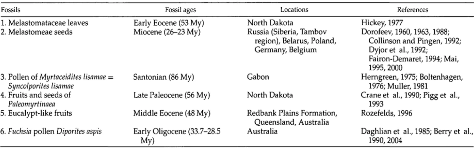
TABLE 1. Fossils used in this study with corresponding ages, locations, and references. Fossils

1. Melastomataceae leaves 2. Melastomeae seeds

3. Pollen of Myrtaceidites lisamae = Syncolporites lisamae

4. Fruits and seeds of Paleomyrtinaea 5. Eucalypt-like fruits 6. Fuchsia pollen Diporites aspis

Fossil ages Early Eocene (53 My) Miocene (26-23 My)

Santonian (86 My) Late Paleocene (56 My) Middle Eocene (48 My) Early Oligocene (33.7-28.5

My)

Locations North Dakota

Russia (Siberia, Tambov region), Belarus, Poland, Germany, Belgium

Gabon North Dakota

Redbank Plains Formation, Queensland, Australia Australia

References Hickey, 1977

Dorofeev, 1960,1963,1988; Collinson and Pingen, 1992; Dyjor et al., 1992;

Fairon-Demaret, 1994; Mai, 1995,2000

Herngreen, 1975; Boltenhagen, 1976; Muller, 1981

Crane et al., 1990; Pigg et al., 1993

Rozefelds, 1996

Daghlian et al., 1985; Berry et al., 1990,2004

rooted using representatives of Lythraceae, i.e., Duabanga grandiflora and Cuphea hyssopifolia, based on the results of global Myrtales analyses (Conti et al., 1996,1997; Sytsma et al., 2004).

DNA Extractions, PCR, Sequencing, and Alignment DNA was extracted as described in Rutschmann et al. (2004) and Schonenberger and Conti (2003). Primers from Zurawski et al. (1981), Olmstead and Sweere (1994), Baum et al. (1998), Bult et al. (1992), and Ku-zoff et al. (1998) were used to amplify and sequence

rbcL, ndhF, r/?/16-intron, nrl8S, and nr26S, respectively.

PCR and sequencing procedures followed the proto-cols described in Rutschmann et al. (2004). The soft-ware Sequencher 4.5 (Gene Codes, Ann Arbor, MI) was used to edit, assemble, and proofread contigs for com-plementary strands. RbcL, nr26S, and nrl8S sequences were readily aligned by eye, whereas ndh¥ and rpll6-intron sequences were first aligned using Clustal X 1.83 (Thompson et al., 1997) prior to final visual adjust-ment with MacClade 4.07 (Maddison and Maddison, 2000).

Phylogenetic Analyses

Plastid (rbcL, ndhF, and r/?/16-intron) and nuclear (n.rl8S, nr26S) partitions were first analyzed separately (results not shown). Because the respective 80% majority-rule consensus bootstrap trees (see below) had no well-supported inconsistencies, plastid and nuclear data sets were combined.

Model selection for each partition was performed in MrAIC 1.4 (Nylander, 2005b), a program that uses PHYML 2.4.4 (Guindon and Gascuel, 2003) to find the maximum of the likelihood function under 24 models of molecular evolution. MrAIC identified the optimal models according to two different selection criteria: the corrected Akaike information criterion (AIC) and the Bayesian information criterion (BIC).

Tree topology and model parameters for each data set were estimated simultaneously using MrBayes version 3.0b4 (Huelsenbeck and Ronquist, 2001; Ronquist and Huelsenbeck, 2003). Bayesian topology estimation used one cold and three incrementally heated Markov chain Monte Carlo chains (MCMC) run for 7 x 106 cycles, with trees sampled every 1000th generation, each using a ran-dom tree as a starting point and the default tempera-ture parameter value of 0.2. For each data set, MCMC runs were repeated twice. The first 5000 trees were dis-carded as burn-in after checking for stationarity on the log-likelihood curves. The remaining trees were used to construct one Bayesian consensus tree and to calculate clade credibility values (Fig. 1).

In addition to the Bayesian clade credibility values (see Fig. 1, numbers below branches), statistical support for individual branches was also calculated by bootstrap re-sampling using the Perl script BootPHYML 3.4 (Nylan-der, 2005a; see Fig. 1, numbers above branches). This program first generates 1000 pseudoreplicates in SEQ-BOOT (part of Phylip 3.63; Felsenstein, 2004), then

per-forms a maximum likelihood analysis in PHYML (Guin-don and Gascuel, 2003) for each replicate under the se-lected model of evolution, and finally computes a 80% majority rule consensus tree by using CONSENSE (also part of the Phylip package).

Branch lengths (see Fig. 1) were estimated, based on the topology of the Bayesian consensus tree, by using the program estbranches as part of the multidivtime Bayesian molecular dating procedure (see below).

Molecular Dating Analyses

All dating analyses described below were performed with multidivtime (Kishino et al., 2001; Thorne et al., 1998; Thorne and Kishino, 2002), which uses an MCMC pro-cedure to derive the posterior distributions of rates and times. For the present study, it was important that

multi-divtime allows for multiple calibration windows (in our

case six calibration points) and different substitution pa-rameters for each data partition (in our case five different partitions).

The analytical procedure followed the steps described in the "Bayesian dating step-by-step manual" (version 1.5, July 2005; Rutschmann, 2005) and included max-imum likelihood branch length optimization with the program estbranches (see Fig. 1). In the last step of the dating procedure (see Rutschmann, 2005), the follow-ing prior distributions were specified (in units of 10 My, as suggested in the manual): RTTM = 12, RTTMSD = 3, RTRATE and RTRATESD = 0.00815, BROWNMEAN and

BROWNSD = 0.0833, and BIGTIME = 13. The first two

values, which define the mean and the standard devi-ation of the prior distribution for the age of the root, were chosen in light of published estimates for the age of the Myrtales crown group (100 to 107 My, Wikstrom et al., 2001,2003; 105 My, Magall6n and Sanderson, 2005; and 111 My, Sytsma et al., 2004; see also Sanderson et al., 2004). The value for BIGTIME was chosen in order to re-flect the estimated age of the oldest eudicot pollen (Doyle and Donoghue, 1993). The age of the eudicots (about 125 My) is one of the firmest dates from the fossil record because of the numerous reports of fossil tricolpate pollen, with no tricolpate pollen appearing before this time.

We ran the Markov chain for at least 5 x 105 cycles and collected one sample every 100 cycles, without sampling the first 8 x 104 cycles (burn-in sector). Initial experi-ments with 2 x 106 cycles showed no differences, leading us to the conclusion that convergence was reached much earlier. We performed each analysis at least twice with different initial conditions and checked the output sam-ple files to assure convergence of the Markov chain by using the program Tracer 1.3 (Rambaut and Drummond, 2005).

The detailed procedure of fossil selection and assign-ment to alternative nodes for calibration of the molecular clock is described in Appendix 1. Briefly, six fossils were chosen, five of which could be attached to alternative calibrations nodes, for a total of 72 possible calibration sets.

Finding the Most Internally Consistent Calibration Sets by Using Fossil Cross-Validation

To evaluate whether some of the 72 calibration sets were more internally consistent than others, we imple-mented the fossil cross-validation procedure of Near and Sanderson (2004) and Near et al. (2005b). Whereas these authors developed the method to identify possibly in-consistent points in a single calibration set, we expanded their approach to compare the internal consistencies of different calibration sets generated by alternative nodal assignments of multiple fossils. Therefore, for each of the 72 calibration sets in our case study, we performed the following steps:

1. We fixed one out of the six calibration points and es-timated the ages of the remaining five unconstrained nodes.

2. For each unconstrained node, we then calculated the difference D, between its estimated and its fossil age. This difference was defined by Near and Sanderson (2004) as an absolute deviation measure D, = (esti-mated age - fossil age). Instead, we used the rela-tive deviation measure D, = (estimated age - fossil age)/fossil age), as suggested in Near et al. (2005b). 3. Then, we calculated SSx, the sum of the five squared

D, values (by using equation 2.2 in Near and Sander-son, 2004).

4. The procedure described above (steps 1 to 3) was then repeated 5 times, each time by fixing a different cali-bration point.

5. Based on the six SSx scores obtained above, we cal-culated the average squared deviation s for the entire calibration set (with equation 2.3 in Near and Sander-son, 2004; see Table 2).

By using this procedure iteratively, we obtained s val-ues for all 72 calibration sets. High valval-ues of s would indicate that one or more calibration points in a set are inconsistent with the others, suggesting that the corsponding fossils were erroneously assigned to the re-spective nodes, whereas low s values would characterize calibration sets with high internal consistency.

In order to account for possible effects related to the molecular dating method (in our case multidivtime), the cross-validation experiments were repeated by using pe-nalized likelihood (Sanderson, 2002) implemented in r8s (Sanderson, 2003; data not shown). For batch processing the calculations of SSx a nd s, we wrote a collection of Perl scripts (available from the first author upon request).

Relationship between Average Squared Deviation s and Nodal Distance

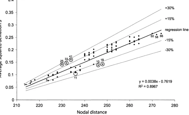
Because the fossil cross-validation procedure might be influenced by the position of the calibration points rela-tive to each other (Near et al., 2005a), we tested whether the average squared deviations sof the 72 calibration sets were correlated with the number of nodes separating the points of a calibration set (nodal distance; Fig. 2). For

each calibration set, the total nodal distance was calcu-lated by adding all pairwise nodal distances between each fixed calibration node and each of the five uncon-strained nodes (step 1 of the fossil cross-validation; see above) and then summing up over all calibrations (step 4 of the fossil cross-validation). This calculation of to-tal nodal distance thus reflects the goal of the present study; i.e., comparing the global internal consistencies among entire calibration sets (see Table 2). Correlation significance was tested by using the F -test statistic un-der a linear regression model in R (R Development Core Team, 2004). Because the 72 calibration sets differed in their degree of correlation between average squared de-viation s and nodal distance (Fig. 2), we also calculated the percent deviation of s from the regression line with nodal distance for each calibration set (see Table 2) and plotted the results as a histogram (Fig. 3). The percent deviation of s represents a corrected measure of internal consistency among the calibration points of a set, termed "corrected calibration-set consistency" from now on.

Effect of Corrected Calibration-Set Consistency on Dating Precision

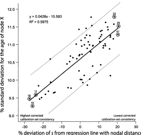
In order to check whether there is a relationship be-tween the corrected calibration-set consistency and the precision of the dating estimates for the node of interest (node X; see Fig. 1), we plotted the percent standard de-viation for the age of node X calculated for each of the 72 calibration sets (see below) against the percent devia-tion of s from the regression line with nodal distance (see Table 2; Fig. 4). Correlation significance was then tested with an F -test statistic under a linear regression model inR.

RESULTS

Phylogenetic Analyses

The data sets used for the phylogenetic analy-ses contained a total of 5124 aligned positions or characters (chars) for 74 taxa, comprising three plas-tid and two nuclear partitions: rbcL (1144 chars),

ndh¥ (818 chars), rp/16-intron (560 chars), nrl8S (1634

chars), and nr26S (968 chars; see online appendix at http://systematicbiology.org for GenBank accession numbers and TreeBASE study accession number SI 775 for data matrix and tree definition). The optimal mod-els of molecular evolution selected by MrAIC (Ny-lander, 2005b) were: SYM+I+G for rbcL, GTR+G for

ndhF, GTR+G for rp/16-intron, SYM+I+G for nrl8S, and

GTR+I+G for nr26S. In all cases, the AICc and BIC cri-teria applied in MrAIC (Nylander, 2005b) selected the same models.

The MrBayes majority-rule consensus tree, including maximum likelihood branch lengths (optimized in

es-tbranches), maximum likelihood bootstrap support

val-ues (estimated in BootPHYML 3.4), and Bayesian clade credibility values (calculated in MrBayes), is shown in Figure 1. The tree topology is congruent with pub-lished phylogenies (Conti et al., 2002; Renner, 2004;

0.4 0.35

I

0.3

'5 0.25

3

FIGURE 2. Correlation between the average squared deviation s and nodal distance among calibration points for each calibration set (see Table 2). R represents Pearson's correlation coefficient. Calibration sets 1, 9, 5 and 50, 66, 58 represent the sets with the lowest and highest s values, respectively. Calibration sets 18,10,11 and 33,41,25 (circled) show the s values that deviate the most below and above the regression line, respectively. The dotted lines above and below the regression line mark a deviation of ±15% and ±30% from the regression line, respectively.

Rutschmann et al., 2004; Schonenberger and Conti, 2004; Sytsma et al., 2004; Wilson et al., 2005). The well-supported Southeast Asian Crypteroniaceae are sis-ter to a clade formed by the Central /South American Alzateaceae and the African Rhynchocalycaceae, Olini-aceae, and Penaeaceae. Memecylon is weakly supported as sister to Melastomataceae, corroborating the phyloge-nies of Clausing and Renner (2001) and Renner (2004). Within Melastomataceae, Melastomeae, Miconieae, and Merianieae are well supported as monophyletic. Within Myrtaceae s.l., Psiloxyloideae are sister to the rest of the clade, referred to as Myrtaceae s.s. (syn. Myrtoideae), in agreement with the phylogeny of Wilson et al. (2005). Myrteae, Melaleuceae, Eucalypteae, and Leptospermeae are all monophyletic, as in Wilson et al. (2005). The posi-tion of Vochysiaceae sister to Myrtaceae s.l. confirms the results of Sytsma et al. (2004) and Wilson et al. (2005). The relationships among the sampled Onagraceae are resolved as in Berry et al. (2004), Conti et al. (1993), and Levin et al. (2003).

Finding the Most Internally Consistent Calibration Sets by Using Fossil Cross-Validation

The five steps to calculate the average squared devi-ations (s values) were performed for all 72 calibration sets within 24 h by using two personal computers with

3-GHz Intel Pentium IV processors simultaneously. The s scores calculated in the fossil cross-validation analyses ranged from 0.061 (with calibration set 1) to 0.265 (with calibration sets 50 and 66; Table 2). The lowest s score was generated by the calibration set where all six fos-sils were assigned to stem nodes, whereas the highest s score was produced by a set with most fossils assigned to crown nodes (Table 2). The use of penalized likelihood (implemented in r8s) instead of Bayesian dating (imple-mented in multidivtime) to estimate divergence times did not affect the s scores substantially; i.e., the ranking of the s scores remained unchanged (data not shown).

Relationship between Average Squared Deviation s and Nodal Distance

The linear regression between the average squared de-viations s of the 72 calibration sets and the distances in number of nodes between the calibration points of each calibration set produced an R2 of 0.8967 (Fig. 2). The F-test statistic showed a significant correlation (degrees of freedom 1 and 70; P < 2.2 x 10"16). The three calibra-tion sets with the lowest s values were 1,9, and 5 (Fig. 2, left), while the three sets with the highest s values were 50,58, and 66 (Fig. 2, right).

Twelve calibration sets had s values at least 10% lower than expected based on the regression line with nodal

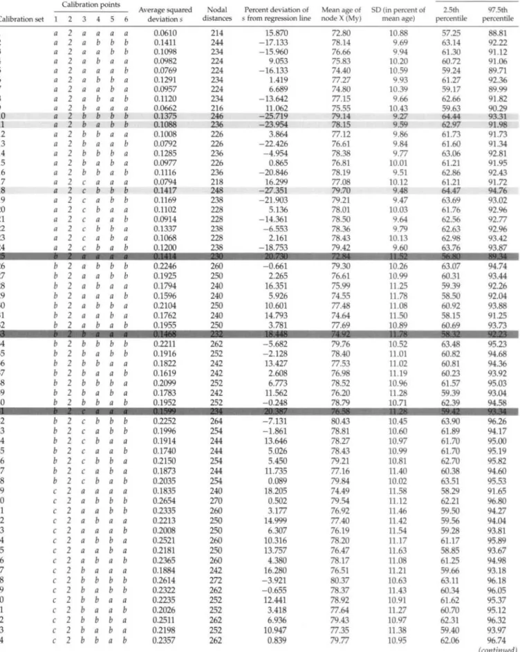
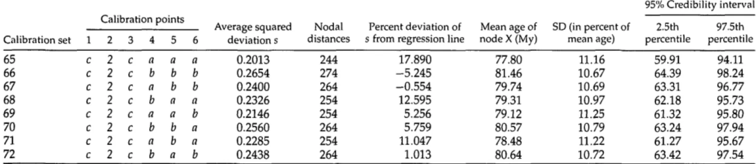
TABLE 2. Characteristics of the 72 different calibration sets, each consisting of six calibration points: Average squared deviation s (see Fig. 2); nodal distances summed up over all fossil cross-validation steps (see Fig. 1); percent deviation of s from regression line with nodal distances (see Fig. 3); mean ages of node X (see Fig. 1) with percent standard deviations and 95% credibility intervals (see Fig. 4). The three sets with the highest level of corrected calibration-set consistency are shaded in light grey, whereas the three sets with the lowest corrected consistency are shaded in dark grey (see Fig. 3). Note that fossil 2 could be assigned to only one node in our phylogeny (node 2).

Calibration set 1 2 3 4 5 6 7 8 9 10 11 12 13 14 15 16 17 18 19 20 21 22 23 24 26 27 28 29 30 31 32 34 35 36 37 38 39 40 1 a a a a a a a a a a a a a a a a a a a a a a a a b b b b b b b b b b b b b b Calibration points 2 2 2 2 2 2 2 2 2 2 2 2 2 2 2 2 2 2 2 2 2 2 2 2 2 2 2 2 2 2 2 2 2 2 2 2 2 2 2 3 a a a a a a a a b b b b b b b b c c c c c c c c a a a a a a a b b b b b b b 4 a b a b a b a b a b a b a b a b a b a b a b a b b a b a b a b b a b a b a b 5 a b b a a b b a a b b a a b b a a b b a a b b a b b a a b b a b b a a b b a 6 a b b a b a a b a b b a b a a b a b b a b a a b b b a b a a b b b a b a a b Average squared deviation s 0.0610 0.1411 0.1098 0.0982 0.0769 0.1291 0.0957 0.1120 0.0662 0.1375 0.1088 0.1008 0.0792 0.1285 0.0977 0.1116 0.0794 0.1417 0.1169 0.1102 0.0914 0.1337 0.1068 0.1200 0.2246 0.1925 0.1794 0.1596 0.2104 0.1762 0.1955 0.2211 0.1916 0.1822 0.1619 0.2099 0.1783 0.1952 Nodal distances 214 244 234 224 224 234 224 234 216 246 236 226 226 236 226 236 218 248 238 228 228 238 228 238 260 250 240 240 250 240 250 262 252 242 242 252 242 252 Percent deviation of s from regression line

15.870 -17.133 -15.960 9.053 -16.133 1.419 6.689 -13.642 11.062 -25.719 -23.954 3.864 -22.426 -4.954 0.865 -20.846 16.299 -27.351 -21.903 5.136 -14.361 -6.553 2.161 -18.753 -0.661 2.265 16.351 5.926 10.601 14.793 3.781 -5.682 -2.128 13.427 2.608 6.773 11.562 -0.248 Mean age of node X (My) 72.80 78.14 76.66 75.83 74.40 77.27 74.80 77.15 75.55 79.14 78.15 77.12 76.61 78.38 76.81 78.19 77.08 79.70 79.21 78.01 78.50 78.36 78.43 79.42 79.30 76.61 75.99 74.55 77.48 74.64 77.69 79.76 78.40 77.53 76.98 78.52 76.20 78.79 SD (in percent of mean age) 10.88 9.69 9.94 10.20 10.59 9.93 10.39 9.66 10.43 9.27 9.59 9.86 9.84 9.77 10.01 9.51 10.12 9.48 9.47 10.03 9.64 9.79 10.13 9.60 10.26 10.99 11.25 11.78 11.08 11.50 10.89 10.52 11.01 11.02 11.19 10.96 11.28 10.71 95% Credibility interval 2.5th percentile 57.25 63.14 61.30 60.72 59.24 61.27 59.17 62.66 59.63 64.44 62.97 61.73 61.60 63.06 61.21 62.86 61.21 64.47 63.69 61.76 62.56 62.63 62.98 63.76 63.07 60.31 59.39 58.50 60.92 58.15 60.69 63.48 60.82 60.81 60.23 61.57 59.39 62.39 97.5th percentile 88.81 92.22 91.12 91.06 89.71 92.36 89.99 91.82 90.29 93.31 91.98 91.73 91.34 92.81 91.95 92.43 91.72 94.76 93.02 92.96 92.77 92.96 93.42 93.87 94.74 93.44 92.26 92.04 93.88 91.25 93.73 95.23 94.68 94.36 93.92 95.03 93.04 94.58 42 43 44 45 46 47 48 49 50 51 52 53 54 55 56 57 58 59 60 61 62 63 64 b b b b b b b c c c c 2 c 2 c 2 c 2 c 2 c 2 c 2 c 2 c 2 c 2 c 2 c 2 c 2 a a a b a a a b a a a b a a a b b a b b b a b b b a b b b a b b b b b b a a a b b a b a a b a a b b b b a a a b b a b a a b a a b b b b a a a b b a b a a b 0.2252 0.1996 0.1914 0.1740 0.2150 0.1873 0.2035 0.1835 0.2654 0.2335 0.2213 0.2008 0.2521 0.2181 0.2365 0.1884 0.2614 0.2322 0.2235 0.2026 0.2511 0.2198 0.2357 264 254 244 244 254 244 254 240 270 260 250 250 260 250 260 242 272 262 252 252 262 252 262 -7.131 -1.861 13.646 5.026 5.450 11.735 0.089 18.205 0.502 3.177 14.999 6.307 10.316 13.757 4.380 16.280 -3.921 -0.655 12.441 3.418 6.936 10.947 0.839 80.43 78.81 78.27 78.43 79.21 77.16 79.84 74.49 79.54 76.92 77.40 76.19 78.20 76.47 78.17 76.51 80.37 78.37 78.92 77.64 79.43 77.35 79.77 10.45 10.60 10.97 10.99 10.81 11.40 10.02 11.58 11.12 11.46 11.42 11.54 11.17 11.63 11.08 11.21 10.63 11.43 10.91 11.27 10.97 11.38 10.95 63.90 61.89 61.70 61.70 62.70 60.38 63.51 58.29 62.21 59.50 59.56 59.28 61.17 58.85 61.25 59.66 63.11 60.34 61.62 60.70 62.31 59.40 62.06 96.26 94.17 95.00 95.19 95.82 94.60 95.53 91.65 96.80 94.27 94.04 93.81 95.89 93.67 94.98 93.18 96.18 96.05 95.37 95.12 96.32 93.97 96.74 (continued)

TABLE 2. Characteristics of the 72 different calibration sets, each consisting of six calibration points: Average squared deviation s (see Fig. 2); nodal distances summed up over all fossil cross-validation steps (see Fig. 1); percent deviation of s from regression line with nodal distances (see Fig. 3); mean ages of node X (see Fig. 1) with percent standard deviations and 95% credibility intervals (see Fig. 4). The three sets with the highest level of corrected calibration-set consistency are shaded in light grey, whereas the three sets with the lowest corrected consistency are shaded in dark grey (see Fig. 3). Note that fossil 2 could be assigned to only one node in our phylogeny (node 2).

Calibration set 65 66 67 68 69 70 71 72 1 c c c c c c c c Calibration points 2 2 2 2 2 2 2 2 2 3 c c c c c c c c 4 a b a b a b a b 5 a b b a a b b a 6 a b b a b a a b Average squared deviation s 0.2013 0.2654 0.2400 0.2326 0.2146 0.2560 0.2285 0.2438 Nodal distances 244 274 264 254 254 264 254 264 Percent deviation of s from regression line

17.890 -5.245 -0.554 12.595 5.256 5.759 11.047 1.013 Mean age of node X (My) 77.80 81.46 79.74 79.31 79.12 80.57 78.48 80.64 SD (in percent of mean age) 11.16 10.67 10.69 10.97 11.25 10.79 11.22 10.72 95% Credibility interval 2.5th percentile 59.91 64.39 63.31 62.18 61.32 63.24 61.27 63.42 97.5th percentile 94.11 98.24 96.77 95.73 95.80 97.94 95.67 97.54

distance (termed "calibration sets A" from now on; see Fig. 3, left side). In all 12 sets, fossil 1 was always as-signed to node la, and fossil 6 to node 6b, whereas the nodal assignments of fossils 3, 4, and 5 varied (Table 3). More specifically, calibration sets 18, 10, and 11 (Fig. 2) showed the s values that deviated the most below the regression line (-27.35%, -25.72%, and -23.95%, respectively; Table 2 and Fig. 3). Based on these results, we conclude that these three sets are char-acterized by the highest level of internal consistency corrected for nodal distance (corrected calibration-set consistency). Experiments of sequential removal of cal-ibration points from each of calcal-ibration sets 18, 10, and 11, following the procedure by Near and Sander-son (2004), never produced a statistically significant decrease of the average squared deviation s between estimated and fossil ages (significance level set at P = 0.01; figure available online at http://systematicbiology. org), indicating that no calibration points should be removed from the most consistent calibration sets.

Twenty-three calibration sets were associated with s values that were at least 10% higher than expected from the regression line (Fig. 3, right side; named "calibration sets B" from now on). More specifically, calibration sets 33, 41, and 25 (Fig. 2) showed the s values that devi-ated the most above the regression line (18.45%; 20.39%; 20.73%, respectively; Table 2 and Figure 3). Based on these results, we conclude that these three calibration sets are characterized by the lowest level of internal consis-tency corrected for nodal distance (corrected calibration-set consistency).

Effect of Corrected Calibration-Set Consistency on Dating Precision

The correlation between the corrected measure of calibration-set consistency (defined as percent deviation of s from the regression line with nodal distance) and the percent standard deviation for the age of node X was sig-nificant (Fig. 4). Linear regression resulted in a multiple

R2 of 0.5975, and the F-test statistic showed a signifi-cant correlation (degrees of freedom 1 and 70; P < 1.788

x 10~16). The three calibration sets 18, 10, and 11 pro-duced lower standard deviations for the age of node X than the three calibration sets 33,41, and 25 (Table 2 and Fig. 4).

DISCUSSION

To our knowledge, this is the first study that explores the application of fossil cross-validation to the problem of nodal assignment for selected fossils. Although we realize that the results presented here by no means rep-resent a panacea to the complex challenges of calibra-tion (Magall6n, 2004; Miiller and Reisz, 2005; Near and Sanderson, 2004; Reisz and Muller, 2004; Wray, 2001), we nevertheless hope that our approach is useful when uncertainty exists on the placement of fossils to specific calibration nodes.

Despite well-founded theoretical guidelines (Doyle and Donoghue, 1993; Hennig, 1969; Magall6n, 2004; Patterson, 1981; Sanderson, 1998), it is often difficult in practice to determine the exact phylogenetic place-ment of fossils on the basis of their morphological traits (Doyle and Donoghue, 1992; Manchester and Hermsen, 2000). The uncertainty of nodal assignment might be especially severe for the paleobotanical record, due to the generally lower degree of morphological integra-tion in plants as compared to animals (Donoghue et al, 1989; Doyle and Donoghue, 1987, 1992; Hennig, 1966). Although exhaustive cladistic morphological analyses of extinct and extant taxa should allow for more reli-able attachment of fossils to specific nodes, such anal-yses are rarely available (Donoghue et al., 1989; Doyle and Donoghue, 1993; Hermsen et al., 2003). In most cases, practitioners must depend on published descrip-tions of the morphological features of a fossil, which are often vague and contradictory when it comes to placing it in a phylogeny (Collinson and Pingen, 1992; Hickey, 1977; Manchester and Hermsen, 2000; Pigg et al., 1993; Rozefelds, 1996). Therefore, a careful review of the paleontological literature for a given group of taxa might lead to multiple nodal assignments of a selected fossil that can be equally defended on the basis of morphology.

U C 03 +-» 10 03 T3 O C CD C C

o

.2

72 different calibration sets

4125 33 calibration sets A

V

J

Y

FIGURE 3. Histogram representing the percent deviation of s from the regression line of Figure 2 for all 72 calibration sets. Twelve cal-ibration sets showed s values that were at least 10% lower than expected from the regression line (calcal-ibration sets A). These sets are asso-ciated with the highest level of corrected calibration-set consistency. Twenty-three calibration sets showed s values that were at least 10% higher than expected from the regression line (calibration sets B). These sets are associated with the lowest level of corrected calibration-set consistency.

The possibility of attaching fossils to multiple nodes also depends on the density of taxon sampling in the relevant phylogenetic neighborhood. In many dated chronograms, only one possible assignment exists, be-cause only one taxon was sampled from the perti-nent group (e.g., the assignment of fossil Melastomat-aceae leaves in Conti et al., 2002, or the assignment of fossil Eucalyptoid fruits in Sytsma et al., 2004; see also Sanderson and Doyle, 2001). Although unequivo-cal, this procedure is hardly satisfactory. In the study presented here, we designed taxon sampling in order to allow for multiple nodal assignment possibilities. In fact, five out of the six selected Myrtales fossils (Ta-ble 1) could be justifiably assigned to more than one node, based on the morphological traits discussed in the paleobotanical literature (Collinson and Pingen, 1992; Hickey, 1977; Pigg et al., 1993; Rozefelds, 1996). In total, 72 different assignment combinations (calibration sets) were possible, each comprising six calibration points (Table 2).

Finding the Most Internally Consistent Calibration Sets by Using Fossil Cross-validation

In this study of Crypteroniaceae and related taxa, we use the fossil cross-validation procedure of Near and Sanderson (2004) in a novel way to assess uncertainty in fossil nodal assignment. More specifically, our goal is to identify the most congruent calibration sets by compar-ing the internal consistencies of all 72 calibration sets gen-erated from alternative placements of six fossils (Table 2). Our procedure differs from that described by Near and Sanderson (2004) in one important respect. Their orig-inal implementation of fossil cross-validation relied on SSx values (i.e., sums of squared differences between fos-sil and estimated molecular ages) that were calculated based on a single calibration point (see steps 1 to 3 in Materials and Methods). The SSx values then guided the removal of selected fossils that were in conflict with the other fossils of a multiple calibration set. Therefore, the SSx values utilized for fossil removal were influenced by

X o> •o

o

o

I

% deviation of s from regression line with nodal distance

FIGURE 4. Correlation between corrected calibration-set consistency (expressed as percent deviation of s from the regression line with nodal distance; see Figs. 2 and 3) and percent standard deviation for the age of node X. The three calibration sets 18,10, and 11 produced lower standard deviations for the age of node X than the three calibration sets 33,41, and 25. The dotted lines above and below the regression line represent the 95% prediction interval, the area in which 95% of all data points are expected to fall.

the idiosyncrasies of the single calibration points used in their calculation. Conversely, in our implementation of fossil cross-validation, we calculate the average squared deviation s for an entire calibration set by using all six fossils as calibration points (see steps 4 to 5 in Materials and Methods). We then employ these average s values to compare the internal consistencies of all 72 calibra-tion sets, each one including all six fossils. Therefore, our procedure is less influenced by the peculiarities of individual deviations between the age of the fossil used for calibration during fossil cross-validation and the ac-tual age of nodal divergence for the same calibration point.

The analyses revealed large differences among the av-erage squared deviations associated with the 72 calibra-tion sets, ranging from an s value of 0.061 for set 1 to an

s value of 0.265 for set 66 (Table 2; Fig. 2). Therefore, one

might conclude that the assignment of fossils 1, 2, 3, 4, 5, and 6 to nodes la, 2, 3a, 4a, 5a, and 6a, respectively, produced the most internally consistent calibration set, while the assignment of the same fossils to nodes lc, 2,

3c, 4b, 5b, and 6b, respectively, produced the most

incon-sistent one. However, in calibration set 1 all the fossils are assigned to their stem nodes, while in calibration set 66 all the fossils are assigned to their crown nodes, except for fossil 2, for which only one nodal assignment is

pos-sible (Table 2). It is thus reasonable to ask whether the s values might be influenced by the nodal distance among calibration points. Indeed, a significant positive correla-tion between the average squared deviacorrela-tion s and nodal distances was observed for the calibration sets (Fig. 2).

How can we explain the correlation between s val-ues and nodal distance found in our study? It is impor-tant to remember that the s values are essentially derived from the difference between the estimated and the fos-sil ages of the calibration points in a set. Therefore, one possible interpretation of the observed correlation might

TABLE 3. Distribution of calibration points in calibration sets A (see Fig. 3). The letter x in the "consensus" set indicates that, among the 12 calibration sets, the fossil was assigned to all possible calibration nodes.

Fossil 1 2 3 4 5 6

Nodal assignments in the 12 calibration sets A

a All 12 — 4 6 6 0 Consensus: la 2 b 0 — 4 6 6 All 12 3x 4x 5x 6b c 0 — 4 — — —

relate to the procedures used for nodal age estimation. More specifically, the rate smoothing methods employed in our dating analyses, based on both Bayesian (Thorne et al., 1998) and penalized likelihood (Sanderson, 2002) approaches, allow rates to change between ancestral-descendant branches, thus creating estimation errors that depend on the number of nodes involved in the smooth-ing procedure. Consequently, the greater the nodal dis-tance among calibration points, the greater the possible difference between the estimated and the fossil ages of the calibration points in a set. Because greater nodal dis-tances are associated with sets where fossils are mostly assigned to the corresponding crown nodes (see Fig. 1 and Table 2), this would explain why such sets are char-acterized by greater s values, as in the case of set 66 (Fig. 2). Conversely, calibration sets where most fossils are at-tached to the stem nodes, as in the case of set 1, are as-sociated with smaller nodal distances among calibration points, hence with smaller s values (Fig. 2; Table 2). Thus, our results suggest that the smaller s values associated with calibration sets where most fossils are assigned to stem nodes do not inherently reflect a higher level of con-sistency among the calibration points, but the effects of nodal distance. Therefore, s values appear to represent a biased estimate of internal consistency.

In order to identify the calibration sets least and most affected by nodal distance bias, we ranked all sets ac-cording to the percent deviation of s from the regression line with nodal distance (Fig. 3). This allowed us to rec-ognize calibrations sets 18,10, and 11 as those associated with the highest level of internal consistency corrected for nodal distance, and sets 33, 41, and 25 as those with the lowest level of corrected internal consistency (Table 2). Importantly, the most consistent calibration sets also produced the lowest percent standard deviations for the estimated ages of node X and the least consistent sets the highest percent standard deviations (Fig. 4). This positive correlation might be explained by the observation that inconsistent calibration points in a set contradict each other in their statements about the timing of evolution-ary events, thus producing conflicting estimates for the age(s) of the node(s) of interest, hence higher associated errors (Near and Sanderson, 2004; Near et al., 2005b). Conversely, calibration points in sets with high levels of corrected internal consistency produce convergent esti-mates for the age(s) of the node(s) of interest, hence lower associated errors.

The 12 calibration sets associated with the highest level of corrected internal consistency (Fig. 3, left side) share some common properties. In all, the temporal informa-tion provided by fossil 1 is most consistent with that of the other calibration points if it is assigned to node la (Table 3 and Fig. 1). This result supports the interpreta-tion by Renner et al. (2001) and Sytsma et al. (2004) that the fossil leaves from the Early Eocene of North Dakota (Hickey, 1977) should be assigned to the node represent-ing the entire Melastomataceae crown group, because of the acrodromous leaf venation. On the other hand, fossil 6, representing the pollen Diporites aspis from the Early Oligocene of Otway Basin (Australia; Berry et al.,

1990; Table 1), is most consistent with the other calibra-tion points if it is assigned to node 6b, representing the

Fuchsia crown group (Table 3 and Fig. 1). This

conclu-sion is congruent with the results of molecular dating analyses that produced an age interval for the node cor-responding to 6b compatible with the age of Diporites

aspis (Berry et al., 2004; Sytsma et al., 2004).

No clear pattern emerges from comparisons among calibration sets A for the assignment of fossils 3,4, and 5 (Table 3). However, in the calibration set with the highest level of corrected internal consistency (18; Table 2 and Fig. 5), the three fossils are all assigned to their crown positions (nodes 3c, 4b, and 5b; Fig. 1). Based on this evi-dence, the pollen Myrtaceidites lisamae from the Santonian of Gabon (fossil 3) is most consistently attributed to Myr-taceae s.s. (node 3c), as proposed by Sytsma et al. (2004). Also in agreement with Sytsma et al. (2004), the fruits and seeds of Paleomyrtinaea from the latest Paleocene of North Dakota (fossil 4) are most consistently placed with the crown radiation of the tribe Myrteae (Myrtoideae s.s.; node 4b). Finally, the Eucalypt-like fruits from the Mid-dle Eocene of South Eastern Queensland (fossil 5) are best assigned to the node representing the most recent common ancestor of Eucalyptus and Angophora (node 5b), as suggested by Rozefelds (1996).

In the calibration set with the highest level of corrected internal consistency (18; Table 2 and Fig. 5), four out of the six fossils are attributed to the crown nodes of the relevant clades (3c, 4b, 5b, 6b) and only one to the stem node (la; Fig. 1). Because fossils represent extinct mem-bers of either crown or stem groups (Magallon, 2004), it is not surprising that different fossils in an optimal multicalibration set may be attached to different posi-tions. Despite the seeming simplicity of the conceptual distinction between stem and crown assignments, the ac-tual decision of attaching individual fossils to either the stem or crown node is indeed very complex, because it would require detailed knowledge about the distribution of synapomorphies among extinct and extant taxa (Mag-allon, 2004). Unfortunately, the comprehensive cladistic morphological analyses necessary to achieve a sound at-tribution of fossils to the proper nodes is usually unavail-able (Conti et al., 2004; Magallon, 2004; Near et al., 2005b). Our study thus represents an alternative approach to the difficult decision of fossil nodal assignment.

The Age of Node X and the Biogeographic Origin of Crypteroniaceae

All estimates generated in this study (Table 2) for the mean age of the split between the Southeast Asian Crypteroniaceae and their West Gondwanan sister clade are contained within the interval ranging from 81.5 to 72.8 My. The age estimate derived from the calibration set with the highest level of corrected calibration-set consis-tency (18) is comprised between 72.15 and 87.25 My (Fig. 5). These results are both compatible with and more pre-cise than published age estimates for the same node (106 to 141 My, Conti et al., 2002; 62 to 109 My, Rutschmann et al., 2004). However, it is important to note that the

Dactylocladus stenostachys Crypteronia paniculata Crypteronia borneensis Crypteronia griffithii Crypteronia glabrifolia Axinandra zeylanica Axinandra coriacea Alzatea verticillata Rhynchocalyx lawsonioides Olinia radiata Olinia ventosa Olinia capensis Olinia emarginata Olinia vangueriqides Endonema retziqides Endonema lateriflora Glischrocolla formosa Brachysiphon rupestris Stylapterus fruticulosus Stylapterus ericoides ssp. pallidus Brachysiphon fucatus Penaea acutifolia

Penaea cneorum ssp. gigantea Penaea cneorum ssp. ovate Penaea cneorum ssp. lanceolata Penaea mucronata

Penaea cneorum ssp. cneorum Penaea cneorum ssp. ruscifolia Brachysiphon microphyllus Penaea dahlgrenii Stylapterus ericifolius Stylapterus micranthus Brachysiphon acutus Brachysiphon mundii Saltera sarcocolla Sonderothamnus petraeus Sonderothamnus speciosus Memecylon durum Memecylon edule Pternandra echinata Pternandra caerulescens Rhexia virginica Melastoma beccarianum Tibouchina urvilleana Bertolonia marmqrata Clidemia petiolaris Tococa guianensis Miconia donaeana Meriania macrophylla Graffenrieda latifolia Macrocentrum cristatum Lophostemon confertus Tnstaniopsis sp. indet. Eugenia uniflora Uromyrtus metrosideros Metrosideros excelsa Callistemon citrinus Melaleuca altemifolia Eucalyptus lehmannii Angophora costata Kunzea vestita Leptospermum scoparium Psiloxylon mauritianum Heteropyxis natalensis Vochysia tucanorum Ruizterania albiflora Ludwigia palustris Gaura lindheimeri Oenothera macrocarpa Circaea lutetiana Fuchsia procumbens Fuchsia paniculata Time [mys] Early Late Cretaceous Pal eo ce ne Eocene Oli go ce ne Mio cene P li c n e Tertiary Crypteroniaceae Alzateaceae Rhynchocalycaceae Oliniaceae C and S America Penaeaceae Memecylaceae Melastomataceae Myrtaceae s.l. Vochysiaceae Onagraceae

FIGURE 5. The chronogram derived from the calibration set with the highest level of corrected calibration-set consistency (18; see Table 2). The corresponding calibration points {la, 2, 3c, 4b, 5b, 6b) are marked on the tree.

mentioned studies differed from the one presented here both in gene/taxon sampling and calibration strategies. Despite these differences in the precision of the age esti-mates, the biogeographic scenario most congruent with the timeframes calculated for node X is that the Cryptero-niaceae stem lineage dispersed from Africa to the Deccan plate as the latter drifted northward in relative proximity to the African coast during the Late Cretaceous (approx-imately 125 to 84 Mya; McLoughlin, 2001; Plummer and Belle, 1995). The newly obtained age estimates, then, fur-ther support India's likely role in expanding the range of Crypteroniaceae from Africa to Asia during its north-bound movement along the African coast, corroborating the out-of-India hypothesis for the origin of Crypteroni-aceae (Conti et al., 2002,2004; Moyle, 2004; Rutschmann et al., 2004; see also Lieberman, 2003).

CONCLUSIONS

To summarize, our study illustrates a novel approach to the problem of nodal fossil assignment when equally justifiable alternatives exist. It uses an expanded fos-sil cross-validation procedure to identify the calibra-tion sets with the highest level of internal consistency. After correcting for nodal distance bias, these sets can be used to estimate the ages of the nodes of interest. An important outcome of our study is that the cali-bration sets with the higher corrected internal consis-tency produced lower standard deviations associated with nodal age estimates than sets characterized by lower levels of corrected consistency. The improved precision of the estimate is a desirable property of any analytical tool.

Although we have attempted to suggest a practical approach, based on a modified implementation of avail-able methodology (i.e., fossil cross-validation; Near and Sanderson, 2004; Near et al., 2005b), to address the fun-damental, yet under-studied problem of uncertainty in fossil nodal assignment, we also wish to emphasize that such measures can by no means replace careful review, selection, and evaluation of the fossil record used for calibration. To further improve the procedure of fossil calibration, a multi-pronged approach will be necessary, including comprehensive morphological cladistic anal-yses of extinct and extant taxa (Donoghue et al., 1989; Doyle, 2000; Eklund et al., 2004), estimation of the gap between the time of lineage divergence and the time of first appearance of synapomorphies in the fossil record (Foote and Sepkoski, 1999; Tavare et al., 2002), improved paleontological dating of fossils, and evaluation of the positional effects of calibration nodes in relation to the nodes of interest (Conroy and van Tuinen, 2003; Porter et al., 2005; Smith and Peterson, 2002). Ultimately, the development of methods that incorporate a priori all sources of fossil calibration uncertainty in the procedure of nodal age estimation would represent a real advance-ment towards addressing one of the thorniest problems of molecular dating and improving the accuracy of the estimated ages.

ACKNOWLEDGEMENTS

The staff of the Universiti Brunei Darussalam, the Forestry Depart-ment of Brunei Darussalam, and the Brunei National Herbarium as-sisted in the field and in the laboratory. Jiirg Schonenberger, Marie Frangoise Provost (Fanchon), Fabian Michelangeli, Joan Pereira, Ed Biffin, and Dennis Hansen provided precious leaf material from re-mote places. Sandro Wagen and Daniel Heinzmann generated many sequences in the laboratory. David Greenwood and David Christophel helped with the interpretation of fossils and provided useful citations. Jeff Thorne answered some questions on multidivtime. F.R. was finan-cially supported by the Kanton Zurich, the University of Zurich, and the Claraz-Schenkung in Zurich.

REFERENCES

Alroy, J. 1999. The fossil record of North American mammals: Evidence for a Paleocene evolutionary radiation. Syst. Biol. 48:107-118. Anderson, J. A. R., and J. Muller. 1975. Palynological study of a

Holocene peat and a Miocene coal deposit from NW Borneo. Rev. Palaeobot. Palynol. 19:291-351.

Aris-Brosou, S., and Z. Yang. 2002. Effects of models of rate evolution on estimation of divergence dates with special reference to the metazoan 18S ribosomal RNA phylogeny. Syst. Biol. 51:703-714.

Ashton, P. S., and C. V. S. Gunatilleke. 1987. New light on the plant ge-ography of Ceylon: I. Historical plant gege-ography. J. Biogeogr. 14:249-285.

Baum, D. A., R. L. Small, and J. F. Wendel. 1998. Biogeography and flo-ral evolution of baobabs (Adansonia, Bombacaceae) as inferred from multiple data sets. Syst. Biol. 47:181-207.

Bell, C. D., and M. J. Donoghue. 2005. Dating the Dipsacales: Com-paring models, genes, and evolutionary implications. Am. J. Bot. 92:284-296.

Benton, M. J., and F. J. Ayala. 2003. Dating the tree of life. Science 300:1698-1700.

Berry, P. E., W. J. Hahn, K. J. Sytsma, J. C. Hall, and A. Mast. 2004. Phy-logenetic relationships and biogeography of Fuchsia (Onagraceae) based on noncoding nuclear and chloroplast DNA data. Am. J. Bot. 94:601-614.

Berry, P. E., J. J. Skvarla, A. D. Partridge, and M. K. Macphail. 1990.

Fuchsia pollen from the Tertiary of Australia. Aust. Syst. Bot.

3:739-744.

Boltenhagen, E. 1976. Pollens et spores S6noniennes du Gabon. Cahiers de Micropale'ontologie 17:1-21.

Bossuyt, F., and M. C. Milinkovitch. 2001. Amphibians as indicators of early Tertiary "out-of-India" dispersal of vertebrates. Science 292:93-95.

Brochu, C. A. 2004. Calibration age and quartet divergence date esti-mation. Evolution 58:1375-1382.

Bult, C, M. Kallersjo, and Y. Suh. 1992. Amplification and sequencing of 16/18S rDNA from gel-purified total plant DNA. Plant Mol. Biol. Rep. 10:273-284.

Christophel, D. C, L. J. Scriven, and D. R. Greenwood. 1992. An Eocene megafossil flora from Nelly Creek, South Australia. Trans. R. Soc. S. Aust. 116:65-76.

Clausing, G., and S. S. Renner. 2001. Molecular phylogenetics of Melas-tomataceae and Memecylaceae: implications for character evolution. Am. J. Bot. 88:486-498.

Collinson, M. E., and M. Pingen. 1992. Seeds of the Melastomataceae from the Miocene of Central Europe. Pages 129-139 in Palaeoveg-etational development in Europe (J. Kovar-Eder, ed.) Museum of Natural History, Vienna, Austria.

Conroy, C. J., and M. van Tuinen. 2003. Extracting time from phyloge-nies: Positive interplay between fossil and genetic data. J. Mammal. 84:444-455.

Conti, E., T. Eriksson, J. Schonenberger, K. J. Sytsma, and D. A. Baum. 2002. Early Tertiary out-of-India dispersal of Crypteroniaceae: Ev-idence from phylogeny and molecular dating. Evolution 56:1931-1942.

Conti, E., A. Fischbach, and K. J. Sytsma. 1993. Tribal relationships in Onagraceae: Implications from rbch sequence data. Ann. Missouri Bot. Gard. 80:672-685.