Orientational dependence of optically detected magnetic resonance signals in laser-driven atomic magnetometers

DOI 10.1007/s00340-016-6604-8

Orientational dependence of optically detected magnetic

resonance signals in laser‑driven atomic magnetometers

Victor Lebedev1 _{· Antoine Weis}1

Received: 2 September 2016 / Accepted: 28 November 2016 / Published online: 29 December 2016 © The Author(s) 2016. This article is published with open access at Springerlink.com

resonance (ODMR) have the longest history in the field of atomic magnetometry, and the so-called Mx-magnetometer using a single light beam has proven to be a highly sensitive and robust device. The theoretical modeling of the signals generated by ODMR-based magnetometers is addressed in great detail in a recently published textbook (Chapter 13 in Ref. [3]).

ODMR magnetometers infer the modulus B0=ω0/γF

of the magnetic field vector B0 from the (driven) Larmor

precession frequency ω0 of an atomic vapor’s

magnetiza-tion, where γF is the gyromagnetic ratio of the used atom

(γF/2π≈ 3.5Hz/nT for 133Cs). The precession is driven by a much weaker additionally applied oscillating field B1(t) ,

called the ‘rf-field’. In the standard Mx-magnetometer, a single circularly polarized light beam whose frequency is resonant with an atomic transition is used both to create the medium’s spin polarization by optical pumping [4] and to read out the spin precession signal.

The magnetometric sensitivity of an OM, i.e., the small-est magnetic field change that the device can detect (in a given bandwidth), depends on many parameters, such as the light intensity, the atomic number density, the size of the atomic sample, the spin coherence time, and the ampli-tude of the rf-field. Moreover, the sensitivity critically depends on the relative orientations of the light propagation direction ˆk, the rf-field ˆB1, and the field of interest ˆB0 . The

latter dependencies imply that there are, on the one hand, orientation(s) that optimize the device’s sensitivity, and, on the other hand, orientations (so-called dead-zones) for which the sensitivity vanishes. The quantitative understand-ing of these dependencies is crucial when designunderstand-ing a mag-netometer, be it for a laboratory application in which the orientation ˆB0 of B0 is mostly known a priori, or for field

applications where the knowledge of the dead-zones is of great importance.

Abstract We have investigated the dependence of

lock-in-demodulated Mx-magnetometer signals on the orientation of the static magnetic field B0 of interest. Magnetic

reso-nance spectra for 2400 discrete orientations of B0 covering

a 4π solid angle have been recorded by a PC-controlled steering and data acquisition system. Off-line fits by pre-viously derived lineshape functions allow us to extract the relevant resonance parameters (shape, amplitude, width, and phase) and to represent their dependence on the ori-entation of B0 with respect to the laser beam propagation

direction. We have performed this study for two distinct Mx -magnetometer configurations, in which the rf-field is either parallel or perpendicular to the light propagation direction. The results confirm well the algebraic theoretical model functions. We suggest that small discrepancies are related to hitherto uninvestigated atomic alignment contributions.

1 Introduction

Optically pumped atomic magnetometers, also known as optical magnetometers (OM), are based on resonant mag-neto-optical effects in atomic (usually alkali-metal) vapors [1]. We refer the reader to the comprehensive overview of various OM methods and their applications in Ref. [2]. Magnetometers based on optically detected magnetic

This article is part of the topical collection “Enlightening the World with the Laser” - Honoring T. W. Hänsch guest edited by Tilman Esslinger, Nathalie Picqué, and Thomas Udem. * Simone Colombo

simone.colombo@unifr.ch

1 _{Physics Department, University of Fribourg, Chemin du} Musée 3, CH-1700 Fribourg, Switzerland

The problem of the OM sensitivity’s orientation depend-ence is closely related to the so-called ‘heading error’ that has already been addressed in the very early accounts on optically pumped atomic magnetometers [5]. Several attempts have been made to overcome those fundamental effects and realize dead-zone-free OM [6–10].

The object of the present paper is an experimental verification of the theoretically predicted [3] orientation dependencies of lock-in-detected signals in different Mx -magnetometers of two distinct geometrical configurations, viz., rf-field either parallel or perpendicular to the light’s k -vector. For this, we have developed a computer-controlled experimental setup allowing the rotation of a static mag-netic field vector of constant modulus over the full 4π solid angle. We record magnetic resonance spectra at 2400 dis-crete (θB, φB) orientations of the field, and off-line analy-sis permits then three-dimensional representations of the results.

2 Experimental setup

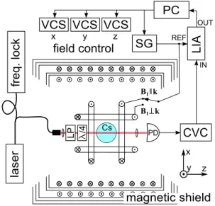
The experimental setup (Fig. 1) is mounted inside of a cubic five-layer µ-metal shield (produced by Sekels GmbH) with inner dimensions of ∼503_cm3_.

The central part of the magnetometer is a spherical (30 mm diameter) Pyrex cell with paraffin-coated inner surface which is connected by a capillary to a reservoir stem containing a droplet of solid cesium producing a

room-temperature saturated atomic vapor [11]. Laser light is guided to the setup by a multimode fiber which effec-tively scrambles the light polarization. The out-coupled (≈2 mm diameter) light beam’s polarization is made cir-cular using a linear polarizer and a quarter-wave plate. We use a polarimeter (Thorlabs, model PAX5710IR1-T) for the precision control of the light’s polarization (cf. Sect. 7.1).

The frequency of the extended cavity diode laser (Top-tica, model DL100 pro) is actively stabilized to the center of the F=4 → F′_{=3 hyperfine transition of the Cs D}

1 line

(=894.6 nm) by means of a separate saturation-absorption spectroscopy unit. The power of the laser beam is kept con-stant by an active stabilization circuit using an intensity modulator (Jenoptik, model AM894) driven by a slow PI controller with a 10 Hz cutoff frequency. The power of the transmitted light beam is detected by a photodiode whose photocurrent is amplified by a current-to-voltage converter (Femto, model DLPCA-200, 106_{V/A gain, 200 kHz}

band-width) and fed to a lock-in detector (Zurich Instruments, model HF2LI).

Magnetic resonance spectra are recorded by automated frequency sweeps of the rf-coil current produced by the built-in oscillator of the lock-in amplifier. The frequency dependence of both the in-phase and quadrature signals obtained by phase-sensitive demodulation of the photodi-ode signal is stored for off-line processing.

The amplifier’s bandwidth and the finite inductivity of the rf-coil imply that the photocurrent’s Fourier component of interest (oscillating at ∼35 kHz) is phase-shifted by a (frequency dependent) value ϕ of ≈20◦ _{with respect to the}

coil-driving voltage.

Data taking is fully computer-controlled by a dedicated LabView code allowing control of the rf-field amplitude and the three components of the offset field B0.

2.1 Magnetic field control and calibration

The static magnetic field inside the shield is produced by a triaxial coil system wound onto the two innermost µ-metal layers. The coils (resistance 4.5 Ω) are driven by voltages from three programmable arbitrary waveform generators (Agilent, model 33500B) via 50 Ω series resistors. After demagnetization, we measure the remnant field compo-nents in the shield using level-crossing (Hanle) resonances as described in Refs. [12, 13]. We nullify these compo-nents—that are typically below 70nT—and calibrate the field producing coils in the following way: For calibrat-ing the Bz coil, we use an Mz geometry, in which we scan

Bz from negative to positive values, while irradiating the atoms with a 1.5kHz rf-field. From the positions of the two magnetic resonances observed in this configuration, we infer both the residual field δBz and the coil calibration con-stant kz. The Bx and By coils are calibrated using a 10µT

Fig. 1 Schematic of the experimental setup. The coils producing the B0 field’s x, y, and z components are wound around the two

inner-most µ-metal layers. Two of the four coils producing Bz are shown as illustration. VCS voltage-controlled current source, SG signal genera-tor, it LIA lock-in amplifier, LP linear polarizer, PD photodiode, CVC current-to-voltage converter, PC computer running control and data acquisition code

offset field (0, B0y, B0z) direction. We measure changes of

the corresponding Larmor frequency

when powering the x- and y- coils individually. Fits allow then to infer kx and ky as well as the residual fields δBx and δBy.

We have observed current scan direction-related (sub-%) differences of the kx and ky constants. These differences may be attributed to the nonlinear ferromagnetic response of the µ-metal onto which the coils are wound. The calibra-tion constant of a given coil may thus be affected by the orientation and the magnitude of the offset field. Based on this, we believe that we control the field orientation at the

1% level.

Using this calibration, the generators are programmed such as to vary the θB- and φB- orientations of the magnetic field vector B0 in a step-wise manner, while keeping the field modulus B0 (nominally) constant. The field is varied

on a full sphere evolving from the north pole (0, 0, B0) to

the south pole (0, 0, −B0) in the coordinates of Fig. 1.

We record magnetic resonance spectra for typically 2400 pairs of discrete values of the field orientation angles (Fig. 2). The duration of each spectrum scan is ≈23 s, so that a complete full-sphere orientation scan (‘θ−φ-scan’) takes ≈15 h.

3 Theory of the

M

The so-called Mx-magnetometer relies on reading out (by optical means) the frequency at which an atomic medium’s spin polarization precesses around a static magnetic field

B0. The precession is coherently driven by a magnetic field (rf-field) of small amplitude B1≪B0 that oscillates at a

frequency ωrf close to the Larmor frequency ω0= γFB0 .

The ensuing phase-synchronized precession of all indi-vidual spins leads to a modulation of the transmitted light power at the frequency ωrf. The amplitude (and phase)

of the induced power modulation depends in a resonant (1)

f0= γF 

(kxIx)2+ (B0y+ kyIy)2+ B20z

manner on the detuning δω ≡ ωrf− ω0 of the rf frequency

from the Larmor frequency. Weis, Grujić ,and Bison have presented an exhaustive discussion of the mathematical expressions for the observed lineshapes in magnetic reso-nance-based atomic magnetometers in a recently published textbook [3].

The simplest Mx-magnetometer implementation uses a single circularly polarized laser beam (in resonance with an atomic transition) that serves for both the creation of the spin polarization and for the readout of the coher-ently driven spin precession. The laser power transmitted through the atomic vapor, which is assumed to be optically thin (κ L ≪ 1), is given by

where P0 is the incident light power and L the length of the

traversed vapor column. The absorption coefficient κ for circularly polarized light depends on the medium’s spin polarization and can be expressed as

where the coefficients α(K)

F,F′ are transition-specific

con-stants, and where κunpol

0 is the absorption coefficient of the

unpolarized medium, Sz and Azz being the medium’s longi-tudinal spin orientation (vector polarization) and alignment (tensor polarization), respectively. Since alignment-related contributions on the 4 → 3 transition studied here are small [14], we will neglect in the following the last term in Eq. (3). The subscript z refers to the quantization axis, cho-sen along the light propagation direction k. In that frame, the longitudinal orientation can be expressed in terms of the sublevel populations pm as

where m is the magnetic quantum number (eigenvalue of

Fz ). In what follows S0 is the value of Sz achieved by opti-cal pumping in a (polarization-stabilizing) magnetic field

B0 oriented along k.

The joint action of the torques exerted by the off-set magnetic field B0 and the oscillating rf-field B_rf(t)_{= B}1ˆB1sin ωrft on the spin polarization causes

a modulation of Sz(t), and hence a time-dependent modulation (2) P_{= P}0exp[−κ L] ≈ P0(1− κ L) , (3) κ _{= κ0}unpol  1_{− α}(1)_F,F′Sz− α(2)_F,F′Azz  , (4) Sz ∝ F  m_=−F pmm, (5) δP(t)_{= P}0κ₀unpolLα_F(1)_,F′Sz(t) (6) ≡ PR(δω) sin[ωrft+ ϕ(δω)] (7) ≡ PIP(δω)sin ωrft+ PQU(δω)cos ωrf

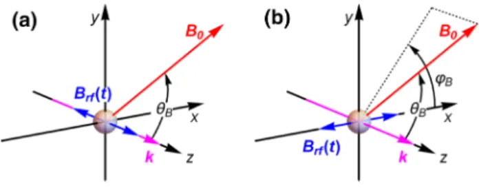
Fig. 2 Definition of the orientation angles θB and φB of the magnetic field in the geometries B1k (a) and B1⊥k (b)

of the transmitted laser power, where δω=ωrf− ω0 is the

rf frequency detuning, and PIP=PRcos ϕ the in-phase and PQU=PRsin ϕ the quadrature amplitude, respectively. As

shown in [3], the power modulation is phase-shifted with respect to the rf-field oscillation by

where the on-resonance phase shift ϕ(0)_{=ϕ(δω=0) depends}

both on the orientation, ˆB1, of the rf-field and on the

orien-tation, ˆB0, of the magnetic field of interest.

We choose ˆz = ˆk as polar axis of a spherical coordi-nates system, so that the magnetic field orientation is deter-mined by the polar and the azimuthal angles, θB and φB, respectively. In this coordinate frame, the amplitude of the detected light power oscillation (‘R’-signal) is given by

where γ is the spin relaxation rate, which is assumed to be isotropic (setting γ =γ1=γ2), and where the signal

calibra-tion factor is given by P_=S0P0κ0unpolLα (1)

F,F′.

As discussed in Ref. [3], all Mx-magnetometer signals can be represented in the form of Eqs. (8) and (9). We therefore refer to these expressions as a ‘universal repre-sentation’ of the Mx-magnetometer signal, whose spectral dependence (but not its absolute value) is independent of the orientation of the rf-field. The interest of writing the phase signal in the universal form lies in the fact that— after electronic subtraction of the offset phase ϕ(0)

depend-ing on ˆB0 and ˆB1—the frequency dependence of the phase

has a pure arctan dependence on the detuning with ϕ=0 on resonance and a negative slope dϕ/dδω.

We define the Rabi frequency associated with the rf-field as Ω=1

2γFB1. Since the component of B1 along B0 does not

induce magnetic resonance transitions, we have introduced in (9) an ‘effective’ Rabi frequency Ω that is associated with the component of B1 that is orthogonal to B0, viz.,

Below we will describe experiments carried out with Mx -magnetometers having two distinct orientations of the rf-field with respect to the light propagation direction, as shown in Fig. 2:

• The B1k geometry shown in Fig. 2a has a cylindrical

symmetry around the k-vector, so that one expects the magnetometer signals only to depend on the polar angle θB. One easily sees that in this case the effective Rabi frequency is given by (8) ϕ(δω)_{= ϕ}  δω_{; ˆB}1, ˆB0  = ϕ(0)ˆB1, ˆB0  − arctanδω_γ , (9) PR(δω)= P  γ2_{+ δω}2 δω2_{+ γ}2_{+ Ω}2 i  Ωi|sin θBcos θB| , (10)  Ω_ˆB 1( ˆ B₀)_{= Ω}    ˆB1−  ˆB1· ˆB0  ˆB0    .

while the on-resonance phase is given by

We note that the offset phase is erroneously given in Ref. [3] (the referred work appeared while preparing the present text) as ϕ(0)

� =0, while the above result is

the correct expression using the 4-quadrant definition of the arctan function for inferring the phase.

• The B1⊥k geometry shown in Fig. 2b is no longer

rota-tionally invariant around k, and it is shown in [3] that in that case one has

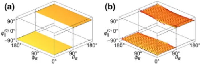
Figure 3 represents the orientation dependencies given by Eqs. (11) and (13).

The on-resonance amplitudes of the R-signals for the two cases (distinguished by the direction ˆB1) are then given

by

4 Data recording

After the careful calibration of the coils generating the x-,

y- and z- components of the field vector B0, we orient the

latter in a systematic manner along 2400 discrete direc-tions, while keeping the field modulus B0 constant. For

this, we feed suitable voltages to the three coils via three series resistors. The voltages are generated by computer-controlled programmable signal generators. A full 4π scan is achieved by varying θB from 0◦ to 180◦ in 40 equidistant (11)  Ω_�(θB, φB)= Ω | sin θB| , (12) ϕ(0)_{� ≡ ϕ}(0)_{ˆz, {θ}B, φB}  = −π 2sign(cos θB). (13)  Ω_⊥(θB, φB)= Ω  cos2_θ B+ sin2θBsin2φB (14) ϕ(0)_{⊥ = ϕ}(0)_{ˆx, {θ}B, φB}  = arctan (cos θBcot φB).

(15) PˆB1 R (0)= ˜P γ Ω_ˆB 1(θB, φB) γ2_{+ Ω}2 ˆB1 (θB, φB) | sin θBcos θB|.

Fig. 3 Anticipated angular dependencies of the effective Rabi fre-quencies Ω_ˆB

steps. For each value of θB, we vary the azimuthal angle φB from 0◦ _{to 360}◦ _{in 60 equidistant steps.}

The field modulus B0 is chosen to be ∼10 µT, which

corresponds to a Larmor frequency f0=_2πω0 of ∼35 kHz.

For each field orientation (θB, φB), we scan the rf frequency ωrf across a range of ±400 Hz (in 8 Hz steps) around the

Larmor frequency ω0. To ensure that the resonance line

is always well centered in the scan range, we do a coarse (automated) determination of the line center after each recording in order to define the start- and stop-frequencies for the scan at the subsequent θB− φB orientation.

Figure 4a shows the spatial distribution of the Larmor frequencies extracted from the off-line analysis of the data discussed in the next section. The average frequency of the displayed points is 36.0(3) kHz. However, we find that during the angular scans the Larmor frequency varies in a systematic manner over a range of ±1 kHz with respect to that average. This variation has an rms value of 0.9% (com-patible with the 1% estimated uncertainty of the calibration constants ki) and is represented in Fig. 4b, where we show the data of Fig. 4a after subtraction of 35.4 kHz.

5 Data analysis

The digital lock-in amplifier records and stores the in-phase and quadrature signals (Cartesian coordinates) as well as the R-signal and phase (polar coordinates). We have dis-covered a synchronous (but phase-shifted) photodiode signal (oscillating at the rf frequency) that is present even in absence of light. We assign this signal to inductive pick-up of the rf-field by the photodiode’s electrical circuit. We have recorded this signal with the laser beam blocked and subtract its in-phase and quadrature components from the corresponding magnetometer signals in the off-line analy-sis. After this correction we calculate the amplitude (PR) and phase (ϕ) signals from the in-phase and quadrature

signals. From the phase signal we subtract the frequency-dependent phase shift of ≈20◦ _{mentioned in Sect. 2.}

Typi-cal results are shown in Fig. 5.

We then fit the theoretical expressions for ϕ(δω) and

PR(δω) given by Eqs. (8) and (9), respectively, to the data. We note that the experimental phase signal is determined by the ratio of the quadrature and the in-phase signals, so that ϕexp(δω) does not depend on the common prefactor of

those signals. We therefore first fit the function

to the experimental phase signals ϕexp(δω). Besides

‘hori-zontal’ (ωfit) and ‘vertical’ (ϕfit(0)) offsets, the shape of the

phase signals is fully determined by the relaxation rates γfit . The fits yield the resonance (Larmor) frequency, ωfit,

the (light power broadened) linewidth, γfit, as well as the

offset phase, ϕ(0)

fit for each field orientation. We note that the

resonance frequencies ωfit determined from such fits are the

values used in Figs. 4.a,b.

Figure 6a shows the angular dependence of the fitted relaxation rates on the field orientation. In Fig. 6b we rep-resent a superposition of the 30 cuts through the sphere of Fig. 6a, one for each of the 30 φB angles. Each given cut (16) ϕfit

ωrf; ωfit, γfit, ϕfit(0)

= ϕfit(0)− arctan

ωrf− ωfit

γfit

Fig. 4 a Angular distribution of the magnetic field modulus B0 as

inferred from the parameters ωfit obtained by fitting the

experimen-tal ϕ(δω) curves with Eq. (16). b The same data, after subtracting ∼10 µT from all moduli, reveal a slight (0.9 %rms) anisotropy of the

distribution 34.2 34.4 34.6 34.8 35.0 0 50 100 150 rf/2 (kHz) PR (mV rms ) 34.2 34.4 34.6 34.8 35.0 100 150 200 250 rf/2 (kHz) (degrees ) (a) (b)

Fig. 5 Typical rf frequency dependence of the amplitude (a) and phase (b) signals of the demodulated detected laser power. Data shown as red points together with fitted functions [Eqs. (17), (16)] shown as solid lines. Data taken with the magnetometer operated in the transverse (B1⊥k) geometry with ˆB0 oriented along θB= 45.67◦, φB= 90◦ and an effective Rabi frequency of Ω= 2.0γ

(a) (b)

Fig. 6 a Angular distribution of the relaxation rates (magnetic reso-nance linewidths) γ /2π as inferred from the parameters γfit obtained

by fitting the experimental ϕ(δω) curves with Eq. (16); b: The same data as a function of θB, with data for all φB values superposed

thus contains 80 γ (θB) points. The average value of all data is γ /(2π)=7.3(4)Hz.

The slight deviation from spherical symmetry observed near the dead-zones occurring at θB=nπ/2 may be due to spin alignment effects addressed in Sect. 7.2. The dead-zones of the alignment contributions occur at different field orientations than those of the orientation contributions and may thus become more prominent when the (otherwise dominant) orientation contribution vanishes. The increased scatter of the data points near these zones is obviously a consequence of the lower signal/noise ratio near these zones.

In the next step, we fit the R-signals by the function

where we have fixed the linewidths γexp to the values γfit

inferred from the phase fits, but leave the resonance fre-quencies ωfit again as free parameters. We note that these

fits yield resonance frequency values ωfit that agree with

those of the phase fits. Those fits also yield the scale factors

Afit and the effective Rabi frequencies Ωfit. Afit is related to

the theoretical amplitude P in Eq. (9) by Afit= η P, where

η is a calibration factor (measured in V/W) that converts laser power levels to recorded voltages.

We have performed the above analysis for all field ori-entations (θB, φB), obtaining a set of on-resonance R-signal values that can be expressed by the fitted parameters via

where γfit results from the fit by Eq. (16) and Ωfit and Afit

from the fit by Eq. (17). We recall that those equations are universal fit functions that can be applied to Mx -magnetom-eter geometries with any orientation of the rf-field.

6 Results

The fit of the magnetic resonance spectrum at each field orientation point (θB, φB) yields the fit parameters ωfit, γfit ,

ϕ_fit(0), Ωfit, Afit as well as the inferred on-resonance signal

amplitude R(0)

fit [defined by Eq. (18)] for each grid point.

This allows graphical representations of the ˆB0 orientation

dependencies of all parameters, the orientation dependence of the applied field modulus having already been shown in Fig. (4).

We complement the latter dependence by showing in Fig7a, b the dependencies of the fitted effective Rabi fre-quencies on the orientation of the field B0 in the B1k and

(17)

Rfit(ωrf; ωfit, Ωfit, Afit)= AfitΩfit

 γ2

exp+(ωrf−ωfit)2

(ωrf− ωfit)2+ γexp2 + Ωfit2

,

(18)

R(0)_fit(θB, φB)≡ Rfit(δω=0) = Afit

γfitΩfit

γ_fit2 ₊Ω_fit2 ,

B_{1⊥k geometries. Note that in the plot we have excluded}

some points near the dead-zones occurring for θB=0◦ , 90◦ , and 180◦ for which the signals vanish in the noise. The results reflect very well the anticipated dependencies shown in Fig. 3.

In view of magnetometric applications, the resonance amplitudes R(0)

fit and the observed linewidths γfit are the

quantities of main interest, since they determine the mag-netometric sensitivity as discussed in Sect. 7.4. While the angular dependence of the relaxation rates has already been

Fig. 7 Measured angular dependencies of the effective Rabi frequen-cies Ωfit for the B1k (a) and B1⊥k (b) geometries. The surface plots

have been obtained by numerical interpolation of ∼2400 discrete data points (some outliers near the dead-zones have been removed). The results are to be compared with the anticipated dependencies shown in Fig. 3

Fig. 8 B1k geometry: Anticipated (a) and measured (b) θB-φB dependencies of the on-resonance phases ϕ(0)

 . The surfaces in the

right graph have been obtained by an interpolation algorithm using the discrete data points (shown as red dots)

Fig. 9 B1k geometry: Theoretical (a) and experimental (b) angular

dependencies of the fitted on-resonance R-signals R(0)

fit for Ω ≈ 2γ.

The solid line on the theoretical graph represents the cut leading to the polar plots shown in Fig. 10

shown in Fig. 6, we will focus in the following subsections on the angular distributions of the R(0)

fit signals, treating

sep-arately the B1k and B1⊥k geometries. 6.1

_B

k

We first address the orientation dependence of the on-res-onance phase ϕ(0)

 . Equation (12) predicts that the ϕ (0)  can

only assume the values −π/2 (for θB< π/2) and +π/2 (for θB> π/2) in the B1k geometry. The experimental findings

shown in Fig. 8 reflect very well this anticipated behavior. In Fig. 9a, b we compare the theoretical prediction and the experimental findings for the R-signal in the B1k

geometry. The plots reflect well the rotational symmetry around the k-direction, and show—at least on the displayed scale—a good qualitative agreement.

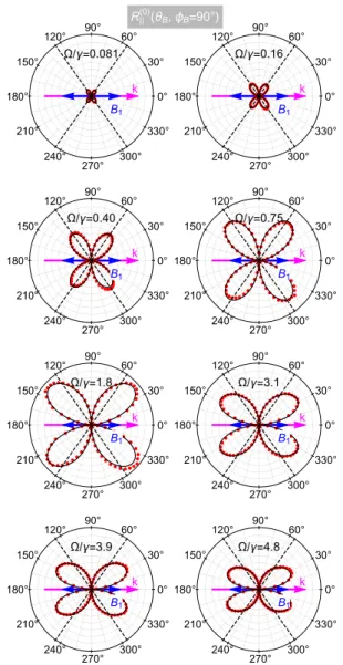
In order to explore the agreement in a more quantita-tive manner, we have performed scans of the θB angle along the trajectory shown in Fig. 9a at a fixed value of φB . The results are shown in Fig. 10. Since the anticipated patterns of R(0)

fit(θB) depend on the rf saturation parameter

Grf= Ω2/γ2, we have measured these dependencies for

different settings of the Rabi frequency Ω, ranging from below-saturation (Ω < γ) to above-saturation (Ω > γ) val-ues. The experimental results are in excellent agreement with theory.

Equations 11 and 15 show that for Ω≪γ the antici-pated θB dependence of the R-signal is given by

Pˆz_R(0)∝| sin2_θ

Bcos θB|, a distribution which has a maxi-mum value at θB∼ 54.7◦. This particular orientation is indicated by dashed lines in the figure. The data points reflect well this behavior. When the Rabi frequency is increased to saturating values Ω ≥ γ, the angular distribu-tion becomes more stretched along the ˆk direcdistribu-tion.

6.2

B

⊥k

We have performed the same type of measurements in the

B_{1⊥k geometry. The magnetometer geometry, determined}

by the orientations ˆk and ˆB1, has no longer a rotational

symmetry axis, and one expects this broken symmetry to be reflected in the orientational dependencies of the mag-netometer signals. The latter obey a reflection symmetry with respect to the plane determined by ˆk and ˆB1.

We start again by addressing first the on-resonance phase, which—because of the broken symmetry—has a non-trivial angular distribution (see Fig. 11). Disregarding some outliers near the dead-zones, which result from large fit errors, the experimental data reflect well the anticipated orientational dependence given by Eq. (14).

The angular dependence of the on-resonance R-sig-nal shown in Fig. 12 exhibits well the broken symmetry

leading to a ‘squeezing/stretching’ along the direction ˆk × ˆB1 . In order to illustrate the broken φB symmetry, we have performed angular scans in which we have varied φB at a fixed angle θB∼ 45◦. The results displayed in Fig. 13a show how the squeezing along ˆB1 evolves into a

stretch-ing along that direction as Ω is increased from below- to above-saturation values.

We also show in Fig. 13b, θB-scans in the plane φB=0 , defined by ˆk and ˆB1 and in Fig. 13c θB-scans in the plane φB=π/2, defined by ˆk and ˆk × ˆB1. Data points are shown

together with theoretical fits (solid lines).

Fig. 10 B1k geometry: Cuts through the angular distributions of

Fig. 9b for φB=90◦ (y–z plane). The polar angle θB is measured with respect to the k axis. The Rabi frequency (expressed in units of γ) is varied from below- to above-saturation values. The red dots are data points and the solid (black) lines represent fits with the model function of Eq. (15). The dashed lines represent the orientation θB at which the low-saturation data are expected to show a maximum sig-nal

7 Discussion

We have investigated in detail the dependence of lock-in detected signals produced by splock-in-orientation (vector magnetization)-based Mx-magnetometers on the orientation of the applied magnetic field of interest B0 and the

orien-tation of the rf-field B1 used to drive the magnetic

reso-nance in the magnetometer. The lock-in signals are fully described by the amplitude (R-signal) and the phase ϕ of the photocurrent oscillation. In all investigated geometries, we find a very good agreement between theoretical predic-tions and our observapredic-tions. We can thus claim a successful verification of the general theoretical expressions for Mx -magnetometer signals that have been presented recently [3].

7.1 Experimental asymmetries

We wish to state nonetheless that achieving the excellent quality of the presented experimental results has been a non-trivial task. One of our goals was to clearly dem-onstrate the anisotropic angular dependence in the two

investigated geometries, viz., the B1k case (rotational

symmetry with respect to ˆk, and reflection symmetry with respect to the plane perpendicular to ˆk), compared to the

B_{1⊥k case which lacks the rotational symmetry while}

keeping the reflection symmetry. In the former case with rotational symmetry, satisfactory results have only been obtained after ensuring that the experimental setup con-tained no symmetry-breaking elements. On our way to the final results, we have identified and successively eliminated the following perturbing effects:

– Even a tiny elliptical polarization of the light beam leads to the creation of transverse alignment (tensor polarization) in the atomic medium that manifests itself in an anisotropic angular distribution. Special care has therefore been taken to ensure the highest possible degree of circular polarization. For the experiments reported in the paper, the light beam (prior to entering the cell) has a degree of linear polarization (DOLP) of 0.70%, which corresponds to a degree of circular polarization (DOCP) of >99.99%. In an earlier experi-ment, we had observed a pronounced anisotropy and discovered later that the light entering the cell in that experiment has had a DOLP of 6%, which corresponded to a DOCP of 99.8%. We note that the DOCP value is given by the corresponding Stokes parameter and that DOCP2+ DOLP2= 1 assuming 100% polarized light. Stress-induced birefringence of the spherical glass cell may slightly alter the light polarization inside of the cell. Any spurious contamination by linear polarization will lead to the creation of transverse spin alignment (tensor polarization), see Sect. 7.2.

– Any magnetic component placed near the Cs vapor cell will perturb the angular distributions in a similar way. We have been able to eliminate such effects by a care-ful choice and screening of all deployed components for magnetic contaminants.

– In an early stage we used rf-coils of rectangular shape (38 × 29 mm2_{, compared to the vapor cell diameter of}

∼30 mm), which led to a pronounced breaking of the rotational φB-symmetry in the B1k geometry.

Replac-ing those coils by 100 mm diameter circular coils has led us to the presented results.

7.2 Alignment effects

Despite the taken precautions, some minor imperfections remain in the data:

(a) A slight (< 1%) anisotropy of the measured Larmor frequencies (Fig. 4b). The maximum quadratic Zeeman shift in the used field of 10 µT is ≪ nT and can thus

Fig. 11 B1⊥k geometry: Anticipated (a) and measured (b) θB-φB dependencies of the on-resonance phases ϕ(0)

⊥. The surfaces in the

right graph have been obtained by an interpolation algorithm using the discrete data points, shown as red dots. The black lines on the left graph indicate B0 orientations for which ϕ(0)_⊥=0. The red dots on the

right graph are data points

Fig. 12 B1⊥k geometry: Theoretical (a) and experimental (b)

angu-lar dependence of the on-resonance R-signals R(0)

fit for Ω ≈ γ. The

reddish and bluish solid lines on the left graph represent the trajecto-ries of the polar plots shown in Fig. 13

be ruled out as cause of the observed deviations at the level of 100 nT.

(b) A slight asymmetry of all recorded R-signals under sat-urating conditions Ω ≥ γ (Fig. 5a).

(c) A slight anisotropy of the relaxation rates γ (Fig. 6b). (d) A slight forward–backward (with respect to k)

asym-metry of the θB scans in the B1k geometry (Fig. 10).

The effect (a) may mainly be assigned to field-dependent calibration constants as discussed in Sect. 4. We believe that the origin of the other effects relies in the following imperfection of the magnetometer model [3]: The model assumes that the atomic medium carries only vector spin polarization, commonly referred to as ‘orientation,’ which, in the language of atomic multipole moments represents a

K_{=1 multipole. It is well known [}1] that optical pumping

with circularly polarized light produces multipole moments

mK,Q of ranks K=1, 2, . . . , 2F (2F=8 in the case of the F_{=4 ground state investigated here), while optical pumping}

with linearly polarized light produces only even multipole moments K = 2, 4, . . . , 2F. It is also known that light inter-acting with the atoms via an electric dipole transition is only sensitive to the rank K = 1 and 2 multipole moments [4].

In view of this, pumping with light of perfect circu-lar pocircu-larization will not only produce a longitudinal (with respect to ˆk) vector polarization (m1,0), but also a longitu-dinal alignment (second rank tensor moment m2,0), whose

contribution has magnetic resonance line shapes and angu-lar distributions that differ from the orientation contributions discussed in the paper. By dropping the last term in Eq. (3), we have explicitly ignored alignment contributions. To our knowledge, the effect of the ignored alignment contribution on the Mx signals has not been discussed in the literature, despite that the Mx-magnetometer has been known for more than half a century. One of the reasons for this may be the fact that for many decades Mx-magnetometers have been operated with discharge lamp light sources, whose broad spectrum does not allow resolving the atomic hyperfine structure, making lamp pumped magnetometers insensi-tive to alignment contributions in J=1/2 atoms, such as the alkalis. We recall that alignment contributions have already been observed in [14] and that they are particularly small on the 4–3 hyperfine components of the D1 line used here. We

are in process of developing a theoretical model allowing us to study this effect in more detail in the near future.

Moreover, the transverse alignment produced by imper-fect circular light polarization is also not included in our model.

7.3 Self‑oscillating magnetometer

We note that the B1⊥k geometry is interesting for realizing a

so-called self-oscillating magnetometer [2], in which the AC

part of the detected photocurrent is used to drive (after suitable amplification and phase shifting) the rf coil. While broadband amplifiers are easy to implement, a broadband phase shifter with fixed amplification is not. We recall that in the B1k

geometry the phase shift ϕ between the photocurrent and the rf-field is ±90◦ _{(Fig. 8), so that a self-oscillating}

magnetom-eter in that configuration will always need a phase shifter. In the B1⊥k geometry, on the other hand, the data of

Fig. 11 show that arbitrary phase shifts ϕ—among them ϕ_{=0—can be achieved. In that geometry, a suitable} orienta-tion of B0 can therefore be used to ensure self-oscillation

without the need of a phase shifter. From Fig. 11, one sees that the phase shift ϕ vanishes for fields B0 lying on the

circle φB= 90◦. The θB orientation on that circle yielding the maximum R-signal depends on the Rabi frequency Ω as illustrated by the graphs in Fig. 13b and shall be chosen appropriately in order to maximize the signal/noise ratio.

One should note, however, that the B1k geometry, in

which the phase is basically independent of the field orien-tation is more reliable in terms systematic readout errors: Changing the orientation of the field will not change the phase and will hence not affect the oscillation frequency. The B1⊥k geometry, on the other hand, offers the

possibil-ity of zero-phase shift operation. However, because of the strongly curved phase vs. orientation surface (Fig. 11), any tilt of the field will change the phase and hence the oscil-lation frequency. The zero-phase advantage can therefore be brought to full profit only in experiments, in which the direction of B0 does not change.

7.4 Magnetometric sensitivity

We end the discussion by addressing the magnetometric sensitivity (or noise-equivalent magnetic field) δBNEM of

the Mx-magnetometer, which can be expressed as

where SNR = R(0)_{/δR denotes the signal/noise}

den-sity ratio, δR being the spectral noise denden-sity of the total detected light power. Since the on-resonance phase slope dϕ/dδω= −γ−1 does not depend on the magnetic field orientation (as supported by our data in Fig. 6), the sensitiv-ity’s angular dependence varies only with R(0)_{. Obviously,}

the larger the amplitude, the higher will be the magneto-metric sensitivity, i.e., the smaller will be the detectable field changes.

From Eq. (15), we conclude that the best magnetomet-ric sensitivity is achieved for θB= 45◦ when the value of | sin θBcos θB| is maximal for both B1 k and B1⊥ k case.

This argument uses the fact that by adjusting Ω one can always ensure that the expression

(19) δBNEM≡ 1 γF 1 SNR     dϕ dδω     −1_δω =0 =_γγ F δR R(0)∝ γ R(0),

(a)

(b)

can be made to reach its maximum value of 1/2 for any φB. Under optimized conditions (θB, φB, Ω) our system has an SNR of 1.5 × 105√_{Hz assuming}

shotnoise-lim-ited detection of the 4 µA DC photocurrent. This yields δBNEM=13 fT/

√

Hz, assuming γ /2π=7 Hz.

8 Outlook

We have demonstrated that our algebraic theory of optically detected magnetic resonances is supported with very good accuracy by experimental observations—at least for the two most commonly deployed configurations of the mag-netometer. An essential result is the now well-understood interdependent effect of the rf-field strength and static field orientation on the resonance amplitudes and phases. This success encourages us to go one step further and to derive a universal algebraic expression that accounts both for an arbitrary orientation (θB, φB) of the static field B0 and—this

will be new—for an arbitrary orientation (θrf, φrf) of the

rf-field B1. Such an expression may be easily adapted to

all-optical designs with Bell-Bloom type of pumping [14–16] as well as to two-beam (pump-probe) experiments. Work in this direction is in progress in our laboratory.

The motivation of the study reported here has been the optimization of an Mx magnetometer in view of reaching the highest sensitivity for measuring B0 (and/or changes

thereof). On the other hand, the Mx principle is also applicable to so-called rf-magnetometry. In that case, a static field B0 of known strength and variable direction is

applied to the sensor, and the task is to measure the ampli-tude and orientation of an unknown rf-field oscillating at a known (or eventually unknown) frequency. ˆB0

orienta-tion scans—as the ones deployed here—can then be used to infer the properties of the rf-field. We have performed preliminary investigations along this direction in the

(20) γ Ω_ˆB 1(θB=45 ◦_{, φB)} γ2_{+ Ω}2 ˆB1(θB=45 ◦_{, φB)}

frame of our ongoing application of atomic magnetometry to the detection of the magnetic response of small (µg) samples of magnetic nanoparticles (MNPs). A problem encountered in such experiments is the detection (in view of minimization) of the stray field from a coil system used to harmonically excite the MNP sample [17, 18]. Details of this research shall be published elsewhere.

Acknowledgements We acknowledge financial support by the Phys-ics Department and the Pool de Recherche of the University of Fri-bourg as well as by Grant No. 200020_162988 of the Swiss National Science Foundation.

Open Access This article is distributed under the terms of the Crea-tive Commons Attribution 4.0 International License ( http://crea-tivecommons.org/licenses/by/4.0/), which permits unrestricted use, distribution, and reproduction in any medium, provided you give appropriate credit to the original author(s) and the source, provide a link to the Creative Commons license, and indicate if changes were made.

References

1. D. Budker, W. Gawlik, D.F. Kimball, S.M. Rochester, V.V. Yash-chuk, A. Weis, Rev. Mod. Phys. 74, 1153 (2002)

2. D. Budker, D.F. Jackson Kimball, Optical magnetometry (Cam-bridge University Press, Cam(Cam-bridge, 2013)

3. A. Weis, G. Bison, Z.D. Grujić, in High Sensitivity

Magnetom-eters, ed. by A. Grosz, M.J. Haji-Sheikh, S.C. Mukhopadhyay Springer, Berlin (2017)

4. W. Happer, Rev. Mod. Phys. 44, 169 (1972) 5. A.L. Bloom, Appl. Opt. 1, 61 (1962)

6. A. Ben-Kish, M.V. Romalis, Phys. Rev. Lett. 105, 193601 (2010) 7. T. Wu, X. Peng, Z. Lin, H. Guo, Rev. Sci. Instr. 86, 103105

(2015)

8. C. Hovde, B. Patton, O. Versolato, E. Corsini, S. Rochester, D. Budker, Heading error in an alignment-based magnetometer, Proc. SPIE 8046, 80460Q (2011)

9. J. Kitching, S. Knappe, V. Shah, P. Schwindt, C. Griffith, R. Jimenez, J. Preusser, L.-A. Liew, J. Moreland, in IEEE

Inter-national Frequency Control Symposium (2008), pp. 789–794 10. E. Breschi, Z.D. Grujić, P. Knowles, A. Weis, Appl. Phys. Lett.

104(2), 023501 (2014)

11. N. Castagna, G. Bison, G. Di Domenico, A. Hofer, P. Knowles, C. Macchione, H. Saudan, A. Weis, Appl. Phys. B 96(4), 763 (2009)

12. N. Castagna, A. Weis, Phys. Rev. A 84, 053421 (2011) 13. E. Breschi, Z.D. Gruijć, A. Weis, Appl. Phys. B 115, 85 (2014) 14. Z.D. Grujić, A. Weis, Phys. Rev. A 88, 012508 (2013)

15. I. Fescenko, P. Knowles, A. Weis, E. Breschi, Opt. Express 21(13), 15121 (2013)

16. E. Breschi, Z.D. Gruijć, P. Knowles, A. Weis, Phys. Rev. A 88, 022506 (2013)

17. S. Colombo, V. Lebedev, Z.D. Grujić, V. Dolgovskiy, A. Weis, Int. J. Magn. Part. Imaging 2, 1606002 (2016)

18. S. Colombo, V. Lebedev, Z.D. Grujić, V. Dolgovskiy, A. Weis, Int. J. Magn. Part. Imaging 2, 1604001 (2016)

Fig. 13 B1⊥k geometry: Cuts through the angular distributions of

Fig. 12b along the trajectories shown in Fig. 12a. Top graphs (a):

R(0)

fit(φB) for θB= π/4; Middle graphs (b): R(0)_fit(θB) for φB= π/2; Bottom graphs (c): R(0)

fit(θB) for φB= 0. In each group of graphs, the Rabi frequency is varied from below- to above-saturation values. The red dots are data points, and the solid black lines represent fits by the model functions. In graphs b and c, the dashed lines represent the field orientations yielding maximum signals in the low-saturation limit