RESEARCH OUTPUTS / RÉSULTATS DE RECHERCHE
Author(s) - Auteur(s) :
Publication date - Date de publication :
Permanent link - Permalien :
Rights / License - Licence de droit d’auteur :
Institutional Repository - Research Portal
Dépôt Institutionnel - Portail de la Recherche
researchportal.unamur.be
University of Namur
Disaggregating census data for population mapping using Random forests with
remotely-sensed and ancillary data
Stevens, Forrest R.; Gaughan, Andrea E.; Linard, Catherine; Tatem, Andrew J.
Published in: PLoS ONE DOI: 10.1371/journal.pone.0107042 Publication date: 2015 Document VersionPublisher's PDF, also known as Version of record Link to publication
Citation for pulished version (HARVARD):
Stevens, FR, Gaughan, AE, Linard, C & Tatem, AJ 2015, 'Disaggregating census data for population mapping using Random forests with remotely-sensed and ancillary data', PLoS ONE, vol. 10, no. 2, e0107042.
https://doi.org/10.1371/journal.pone.0107042
General rights
Copyright and moral rights for the publications made accessible in the public portal are retained by the authors and/or other copyright owners and it is a condition of accessing publications that users recognise and abide by the legal requirements associated with these rights. • Users may download and print one copy of any publication from the public portal for the purpose of private study or research. • You may not further distribute the material or use it for any profit-making activity or commercial gain
• You may freely distribute the URL identifying the publication in the public portal ?
Take down policy
If you believe that this document breaches copyright please contact us providing details, and we will remove access to the work immediately and investigate your claim.
Disaggregating Census Data for Population
Mapping Using Random Forests with
Remotely-Sensed and Ancillary Data
Forrest R. Stevens1*, Andrea E. Gaughan1, Catherine Linard2,3, Andrew J. Tatem4,5
1 Department of Geography and Geosciences, University of Louisville, Louisville, Kentucky, United States of America, 2 Fonds National de la Recherche Scientifique (F.R.S.-FNRS), Rue d’Egmont 5, B-1000 Brussels, Belgium, 3 Biological Control and Spatial Ecology, Université Libre de Bruxelles, CP 160/12, Avenue FD Roosevelt 50, B-1050 Brussels, Belgium, 4 Department of Geography and Environment, University of Southampton, Highfield, Southampton SO17 1BJ, United Kingdom, 5 Fogarty International Center, National Institutes of Health, Bethesda, MD 20892, United States of America
Abstract
High resolution, contemporary data on human population distributions are vital for measur-ing impacts of population growth, monitormeasur-ing human-environment interactions and for plan-ning and policy development. Many methods are used to disaggregate census data and predict population densities for finer scale, gridded population data sets. We present a new semi-automated dasymetric modeling approach that incorporates detailed census and an-cillary data in a flexible,“Random Forest” estimation technique. We outline the combination of widely available, remotely-sensed and geospatial data that contribute to the modeled dasymetric weights and then use the Random Forest model to generate a gridded predic-tion of populapredic-tion density at ~100 m spatial resolupredic-tion. This predicpredic-tion layer is then used as the weighting surface to perform dasymetric redistribution of the census counts at a country level. As a case study we compare the new algorithm and its products for three countries (Vietnam, Cambodia, and Kenya) with other common gridded population data production methodologies. We discuss the advantages of the new method and increases over the ac-curacy and flexibility of those previous approaches. Finally, we outline how this algorithm will be extended to provide freely-available gridded population data sets for Africa, Asia and Latin America.
Introduction
Accurate spatial data sets that represent the distributions of human populations are critical in many health, economic, and environmental fields across various temporal and spatial scales [1–3]. Considering an estimated world population increase of 2.3 billion people between 2011 and 2050, with more than 50% of that growth absorbed into urban areas [4], the ramifications of having accurate population information has never been more important. Demand is increas-ing for more contemporary, easily-updatable population data as research and decision-makincreas-ing a11111
OPEN ACCESS
Citation: Stevens FR, Gaughan AE, Linard C, Tatem AJ (2015) Disaggregating Census Data for Population Mapping Using Random Forests with Remotely-Sensed and Ancillary Data. PLoS ONE 10 (2): e0107042. doi:10.1371/journal.pone.0107042 Academic Editor: Luís A. Nunes Amaral, Northwestern University, UNITED STATES Received: January 27, 2014
Accepted: August 11, 2014 Published: February 17, 2015
Copyright: © 2015 Stevens et al. This is an open access article distributed under the terms of the
Creative Commons Attribution License, which permits unrestricted use, distribution, and reproduction in any medium, provided the original author and source are credited.
Funding: AJT acknowledges funding support from the RAPIDD program of the Science and Technology Directorate, Department of Homeland Security, and the Fogarty International Center, National Institutes of Health, and is also supported by grants from the Bill and Melinda Gates Foundation (#49446 and #1032350). The funders had no role in study design, data collection and analysis, decision to publish, or preparation of the manuscript.
Competing Interests: The authors have declared that no competing interests exist.
become more complex and operates at sub census-unit scales [5,6]. To satisfy this demand searchers are increasingly turning to remotely sensed data and other geospatial data sets to re-fine the process of producing high resolution estimates of population density. But, to make the most of these data sources, new methodologies are needed to more accurately estimate human population distributions.
Gridded population data sets can vary substantially in their depiction of population distri-butions, especially for resource poor countries where recent and detailed census and country-specific geospatial data are often limited [7]. Previous efforts to generate gridded population data sets have utilized areal interpolation techniques, which include basic dasymetric ap-proaches [8] often in conjunction with ancillary data [1] or, alternatively, statistical modeling methods [9]. Widely-used global data sets that rely on an areal weighting scheme include the freely available Gridded Population of the World (GPW) database, versions 2 and 3, and the Global Rural Urban Mapping Project (GRUMP) [8,10]. GRUMP differs from GPW by incor-porating urban-rural designations in the spatial reallocation of population for each census unit [11], primarily derived from satellite nightlights, while GPW is a simple redistribution across census unit. Other large-area population data sets rely on ancillary data to spatially weight pop-ulation density within a given administrative unit. Such data sets include the LandScan Global Population database [12,13], the gridded data sets produced by the United Nations Environ-ment Programme (UNEP) for Latin America, Africa, and Asia [14–16], and the AfriPop and AsiaPop projects which provide freely-available gridded population data for Africa and Asia [5,17–19].
Each of these data products differ in their modeling approach and transparency, the input data and reliability of those data sources, and how input variables interact with each other to determine population distribution. Remotely sensed information has been applied for decades either as the main source for human population estimation [20–22] or alternatively used as a supplementary data source for use in spatially refining census population estimates [17,23– 25]. The use of remotely sensed data is especially important for mapping human population in countries that do not have reliable census data collection [5]. Recent studies focused on map-ping populations in Haiti in 2003, Pakistan in 1998 and Western Kenya in 1999 take advantage of the increased availability of multi-scale remotely-sensed and geospatial data [23,26,27]. These studies use semi-automated classification algorithms combined with a dasymetric map-ping approach for generating fine-scale population data sets. While such studies provide im-portant contributions towards the advancement of accurate gridded population mapping, they can be difficult to apply across regional to continental spatial scales due to a reliance on high resolution imagery that is often expensive to obtain and challenging to process.
Here we propose an approach that complements such methods, with flexibility that allows for incorporating global, large scale data sets of both continuous and discrete covariates when finer scale data do not exist or are difficult to process over large areas. We describe a dasymetric redistribution approach, using population counts from census data and a weighting scheme which is based on a“Random Forest,” nonparametric predictive model [28,29]. The flexibility of this modeling framework allows for the incorporation of remotely sensed and geospatial data from multiple scales into the weighting portion of the dasymetric model. The approach benefits from non-parametric statistical predictions based on the best ancillary data available, but also anchors those predictions across space to the best available, contemporary administra-tive boundary-linked GIS census data.
We present the methodology using case studies of Kenya (KEN), Vietnam (VNM), and Cambodia (KHM). These three countries represent a cross-section of census spatial scales and also reflect the range in ancillary data available for use in the algorithm. We present a
comparison of the population maps and their accuracy for each country with output from the simpler, widely used methods used to create the Afri/AsiaPop, GRUMP and GPW datasets.
Materials and Methods
Data Description
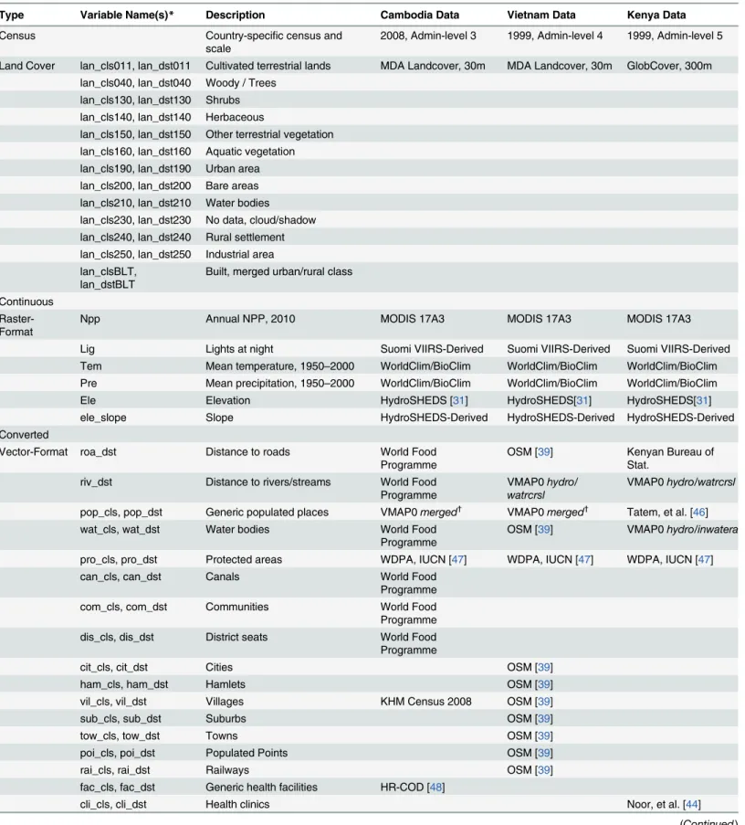
Country-specific census data were collected from the National Institute of Statistics for Cam-bodia, the National Statistics Office in Vietnam, and the National Bureaus of Statistics for Kenya (Table 1). These data were matched to GIS-delineated administrative boundaries for the village (Cambodia), Tinh (Vietnam) and Sublocation (Kenya) levels. These administrative lev-els provided the finest level administrative unit available at the time of analysis. For use in the Random Forest model, the log population density is used as a response variable and this pro-cess is explained in more detail in Section 2.4 with an expanded discussion on the choice of per-forming a log transformation provided in Section 4.3.
Population distribution is often highly correlated with land cover types and we incorporate land cover information using one of two thematic land cover classification data sets. For Cam-bodia and Vietnam, we use EarthSat GeoCover Land Cover Thematic Mapper (TM) data from MDA Federal [30] (Table 1). The GeoCover dataset provides consistent global mapping of 13 land cover classes at a 30-meter spatial resolution and derived from circa 2005 imagery [30]. GlobCover data, which are derived from the ENVISAT satellite mission's MERIS (Medium Resolution Image Spectrometer) imagery, were used for Kenya (Table 1). GeoCover imagery classes were re-coded to be consistent with those land cover classes used by GlobCover and the aggregated classes used in the AsiaPop [19] and AfriPop [25] methodologies. GeoCover data (30 m) were majority aggregated (scaled-up) and GlobCover data (300 m) were resampled (scaled-down) by nearest neighbor to a square pixel resolution of 8.33 x 10⁻⁴degrees (approxi-mately 100 meters at the equator).
Land cover data are complemented by digital elevation data and its derived slope estimates, primarily from the SRTM-based HydroSheds data [31]. We also include MODIS-derived, MOD17A3 estimates of net primary productivity (NPP) [32] as well as observed lights at night, mosaicked from Suomi National Polar-orbiting Partnership (NPP) Visible Infrared Imaging Radiometer Suite (VIIRS) data, standardized and provided as a global coverage [33]. Within-country climatic spatial variation is also incorporated, by using WorldClim/BioClim 1950– 2000 mean annual precipitation (BIO12) and mean annual temperature (BIO1) estimates [34].
In addition to land cover and associated raster data sets, we also include geospatial data that may correlate with human population presence on the landscape such as networks of roads and waterways; large water bodies; settlement or populated place locations; protected area de-lineations; and various“facility” locations (e.g. health clinics, hospitals, schools). The specific data sets available vary widely from country to country, but in almost all cases the most com-prehensive, contemporary datasets that are freely available were used. In the absence of coun-try-specific data for many of these features we extract National Geospatial-Intelligence Agency (NGA) Vector Map Level 0 (VMAP0) data [35]. In many cases the VMAP0 data are the most coarse and non-contemporaneous available, however their world-wide coverage and consisten-cy in level of processing make them a useful base data set, especially in the absence of alterna-tive data for roads, rivers, water bodies and built-up areas. The data used in the case studies presented here are summarized inTable 1.
Data Preparation
The general process used for the data preparation, modeling and validation is outlined in
Table 1. Country-specific data sources and variable names used for population density estimation used for dasymetric weights. Type Variable Name(s)* Description Cambodia Data Vietnam Data Kenya Data Census Country-specific census and
scale
2008, Admin-level 3 1999, Admin-level 4 1999, Admin-level 5 Land Cover lan_cls011, lan_dst011 Cultivated terrestrial lands MDA Landcover, 30m MDA Landcover, 30m GlobCover, 300m
lan_cls040, lan_dst040 Woody / Trees lan_cls130, lan_dst130 Shrubs lan_cls140, lan_dst140 Herbaceous
lan_cls150, lan_dst150 Other terrestrial vegetation lan_cls160, lan_dst160 Aquatic vegetation lan_cls190, lan_dst190 Urban area lan_cls200, lan_dst200 Bare areas lan_cls210, lan_dst210 Water bodies
lan_cls230, lan_dst230 No data, cloud/shadow lan_cls240, lan_dst240 Rural settlement lan_cls250, lan_dst250 Industrial area lan_clsBLT,
lan_dstBLT
Built, merged urban/rural class Continuous
Raster-Format
Npp Annual NPP, 2010 MODIS 17A3 MODIS 17A3 MODIS 17A3 Lig Lights at night Suomi VIIRS-Derived Suomi VIIRS-Derived Suomi VIIRS-Derived Tem Mean temperature, 1950–2000 WorldClim/BioClim WorldClim/BioClim WorldClim/BioClim Pre Mean precipitation, 1950–2000 WorldClim/BioClim WorldClim/BioClim WorldClim/BioClim Ele Elevation HydroSHEDS [31] HydroSHEDS[31] HydroSHEDS[31] ele_slope Slope HydroSHEDS-Derived HydroSHEDS-Derived HydroSHEDS-Derived Converted
Vector-Format roa_dst Distance to roads World Food Programme
OSM [39] Kenyan Bureau of Stat.
riv_dst Distance to rivers/streams World Food Programme
VMAP0 hydro/ watrcrsl
VMAP0 hydro/watrcrsl pop_cls, pop_dst Generic populated places VMAP0 merged† VMAP0 merged† Tatem, et al. [46] wat_cls, wat_dst Water bodies World Food
Programme
OSM [39] VMAP0 hydro/inwatera pro_cls, pro_dst Protected areas WDPA, IUCN [47] WDPA, IUCN [47] WDPA, IUCN [47] can_cls, can_dst Canals World Food
Programme com_cls, com_dst Communities World Food Programme dis_cls, dis_dst District seats World Food Programme
cit_cls, cit_dst Cities OSM [39] ham_cls, ham_dst Hamlets OSM [39] vil_cls, vil_dst Villages KHM Census 2008 OSM [39] sub_cls, sub_dst Suburbs OSM [39] tow_cls, tow_dst Towns OSM [39] poi_cls, poi_dst Populated Points OSM [39] rai_cls, rai_dst Railways OSM [39] fac_cls, fac_dst Generic health facilities HR-COD [48]
cli_cls, cli_dst Health clinics Noor, et al. [44] (Continued )
standalone Python programming language (version 2.6,www.python.org) script that uses the ArcGIS 10.0 SP1 [36] arcpy module and associated extensions for analysis. Slight differences exist in the processing and the data sources used for each country, but these are thoroughly documented in the metadata that accompanies each set of final population maps (see attached
S1 Filefor an example).
Before processing the covariates, the administrative boundary-linked census population count data are converted to raster form by projecting the data into a conformal projection most appropriate for each country (e.g. UTM). Projection is necessary for calculating the dis-tance-to covariates included in the model. The projected census data boundaries, which usually correspond to the national borders of each country, are then buffered by 10 km. This buffered polygon is used in order to minimize edge effects associated with near-border populated areas. The buffered polygon is then converted to a raster grid, with approximately 100 meter by 100 meter pixels, and serves as a template for all other covariates to be projected and subset to for each country.
The vector and raster class-based data, (e.g. individual land cover classes, water bodies, pro-tected area presence/absence, etc.) are first projected and subset to match the buffered national borders. These class data are then converted to binary masks, creating a binary covariate (i.e. “_cls” variables inTable 1). From these masks a distance-to-class raster is calculated for each dataset (i.e.“_dst” variables inTable 1). The one special case for class-based data occurs in the treatment of the“Built” land cover class (“lan_BLT_” inTable 1). Using the same methodology outlined for both the AfriPop and AsiaPop projects [17,19], but using the MODIS 500 m Glob-al Urban Extent product (2001–2002) [37,38], the“Built” class in each land cover dataset is categorized as either“Rural” or “Urban” based on whether the pixel location is within a rural/ urban extent. Furthermore, the built areas may be adjusted on a pixel-by-pixel basis using other ancillary data sources such as OpenStreetMap [39] or country-specific, refined land cover data.
Data sets representing continuously varying properties across the landscape are projected, resampled and aggregated to match the gridded census buffer. These continuous data most often include elevation, slope, spatially explicit climate data, as well as mean annual NPP esti-mates. We also include the best available lights at night data, collected via satellite and mosa-icked into a continuous dataset, subset to each country of interest [33]. Some studies have shown the effects of night light data may be exaggerated due to“light bloom” on neighboring
Table 1. (Continued)
Type Variable Name(s)* Description Cambodia Data Vietnam Data Kenya Data dsp_cls, dsp_dst Dispensaries HR-COD [48] Noor, et al. [44] hos_cls, hos_dst Hospitals Noor, et al. [44] sch_cls, sch_dst Schools HR-COD [48] Kenya Open Data [49] set_cls, set_dst Settlement points World Food
Programme
bui_cls, bui_dst Built land cover Tatem, et al. [46] * The variable names are used in Random Forest model output and throughout the text as reference to the specific data they were derived from. The first three letters are derived from the data type (e.g.“lan” indicates land cover) and the last three letters, if present, indicates what type of data each variable represents (e.g.“_cls” is a binary classification and “_dst” is a calculated Euclidean distance-to variable.
†The default data for populated places is merged from several VMAP0 data sources. There are three VMAP0 data sets used: The point data pop/builtupp
and pop/mispopp are buffered to 100 m and merged with the pop/builtupa polygons creating avector-based built layer. This layer is then converted to binary class and distance-to rasters for use in modeling.
pixels, effects from fires and gas production, and the difficulty of capturing dim but significant light associated with human settlement [40]. While these problems may be significant in a line-ar, parametric modeling context, the approach outlined here is more robust to these types of problems due to the flexible way in which model covariates can interact and influence one an-other. Furthermore, despite problems lights at night is a significant predictor in all models test-ed and so we include it for each country.
Another problem that arises is that many raster data sets are originally acquired at coarser spatial resolution than 100 m, as well as being clipped to overland areas (e.g. WorldClim, MODIS NPP). Once our raster covariates are resampled to match the rasterized census data and its buffer there may be areas with no data at the boundaries, especially on coastal bound-aries. We use a simple nearest neighbor filling approach (the“nibble” tool in ArcGIS 10) to ex-tend the edge of these data sets and fill any gaps prior to model estimation.
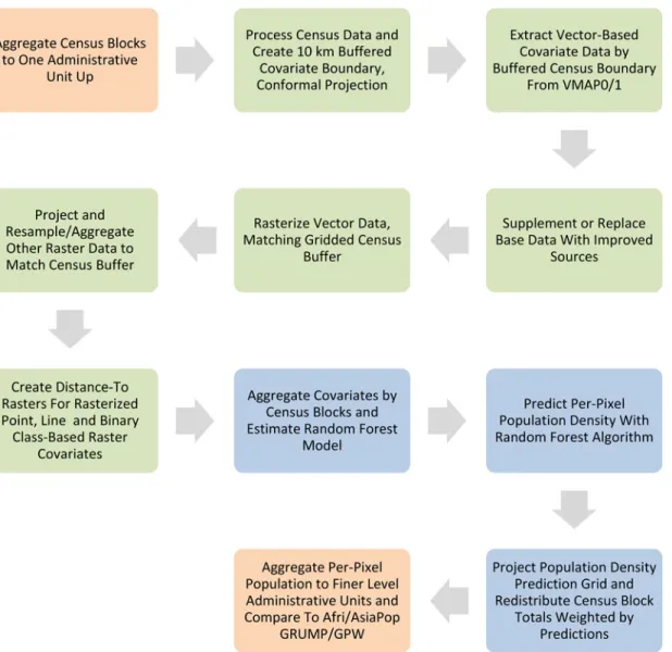
Fig 1. This figure represents the general structure of the data processing and map production procedure used to compare the methodology outlined in this paper to the AfriPop/AsiaPop, GRUMP, and GPW methodologies. The orange boxes represent items that are specific to the research presented here and not part of end-user map data product generation. The green boxes represent data pre-processing stages. Items in blue represent Random Forest model estimation, per-pixel prediction and dasymetric redistribution of census counts.
Population Density Weighting Calculation
The data processing, model estimation and prediction for our algorithm is outlined inFig. 1. For end-user population maps we use the finest level census data available during estimation and population redistribution, with counts adjusted using rural and urban growth rates to esti-mate population distribution for any particular year [25]. However, in these case studies we do not adjust census counts and instead add two steps to the process for comparison purposes (Fig. 1, orange areas). These steps involve aggregating census units to the next administration level up from the finest available. We use these aggregated counts during both estimation and prediction, which then allows us to compare sums from our pixel-level predictions with census counts from the original, fine-scale data. From this we estimate how accurate results may be across spatial scales. In this case study, we aggregated to administrative unit level four ("Divi-sion") for Kenya, and to unit level two ("Province") for Vietnam and Cambodia.
To attain covariate values for each aggregated administrative unit we calculated zonal means for each continuous dataset and counted class majorities for binary data sets. From this process we attained 38 covariates for VNM, 42 for KHM and 44 for KEN. These individual co-variate values were merged with the census count for the aggregated census units, per respec-tive country (Table 1).
Because our aim was to estimate population density for use as a dasymetric weighting layer we must estimate our Random Forest model with a population density“response” variable. Dasymetric redistribution in plain terms is a method to distribute a count representing a sum total (census unit population in this case) across an area (the administrative/census unit). Rath-er than distribute that count equally by area we can use one or more sets of data at a finRath-er spa-tial scale than the administrative unit to unequally weight the redistribution. Ideally this weighting layer(s) better reflects underlying mechanisms contributing to the unequal distribu-tion of the sum of interest.
We calculated the population density within each aggregated administrative unit, dividing the sum of census counts for the year of the census and dividing it by the area of the aggregated blocks. We then removed any census units with zero counts and log-transformed the density in order to create a more normal and even distribution of population density values with respect to our other covariates. Zero count census units are most often associated with protected areas or water bodies that are delineated in the original census data. In many census data sets these may represent a disproportionately large portion of the data and may bias estimation and pre-diction. In testing, eliminating zero count units and using a log transformed population density aids the Random Forest algorithm in finding good splits in the data as the relationship between distance-based covariates and population densities is in most cases more
uniformly distributed.
Weights Model Estimation by Random Forest
The population density and covariate aggregation values for each census unit were then used to create a Random Forest model [28] to predict log population density. Random Forest models are an ensemble, nonparametric modeling approach that grows a“forest” of individual classifi-cation or regression trees and improves upon bagging [41] by using the best of a random selec-tion of predictors at each node in each tree [28,29]. In many cases the predictive performance for Random Forests is on par with boosted regression trees [42] but have the advantage of hav-ing fewer tunhav-ing parameters. In our methodology this is especially important as the tunhav-ing can be automated as part of the fitting process. Furthermore, in the case where there are many cor-related predictors or predictors with a large spectrum of informative value (e.g. some with a lot of information among many with very little) the Random Forest algorithm is attractive because
the output from the forest growing algorithm can be used to estimate post-hoc variable importance measures.
Model estimation, fitting and prediction were all completed using the statistical environ-ment R 2.15.3 [43] and the randomForest package 4.6–7 [29]. To streamline the prediction phase and reduce processing time we developed a multi-stage Random Forest estimation tech-nique (see attachedS2 Filefor further details). This technique first fit a series of models using the randomForest tuneRF function with all available covariates and the log population density of each census administrative unit as the response. The tuneRF function uses a step function to tune the Random Forest mtry parameter. This parameter determines the number of covariates to randomly select and choose from the best covariate for each node during the tree growing process. Prediction accuracies can be sensitive to the mtry parameter and tuneRf uses the mini-mization of out-of-bag-prediction error [29] as an objective function to select an appropriate value for mtry.
The next step in our algorithm is a very conservative covariate selection process for the re-sulting Random Forest. We perform this step in order to reduce the number of total covariates in the final Random Forest model which can significantly speed up per-pixel prediction. We use the resulting forest of trees grown for the tuned mtry value and extract covariate impor-tance scores [29]. For any covariate that has a variable importance score of zero, which indi-cates that after random permutation of the covariate values no decline in mean squared error (MSE) of prediction is observed, we remove it from the list of potential covariates and re-run tuneRF with the reduced set of data. This is iterated until only positive importance scores re-main for every covariate included in the modeling process. This usually converges in only one or two iterations and results in the minimum number of covariates that have even a small amount of predictive capacity, while eliminating covariates that are completely redundant or negatively impact prediction.
The only other tuning parameters required for Random Forest estimation are the number of trees to grow per forest and the number of observations to allow in terminal nodes. The lat-ter controls the complexity of each individual tree in the forest by restricting the number of splits required to partition all of the observed response values with the randomly selected co-variates. Trees are grown to a maximum size where terminal nodes contain at most the number of census units divided by 1000 (rounded to the nearest whole number) or a single observation when there are fewer than 1000. Predictions for the entire forest average the selected individual node by each tree in the forest. The sensitivity of prediction accuracy to these parameters is rel-atively low. Based on multiple experimental runs we observed that 500 trees were sufficient across all combinations and permutations of data to arrive at a stable, minimized out-of-bag (OOB) error of prediction [28]. Furthermore, we allowed the trees to grow maximally, which for typical dataset sizes in the regression context could introduce bias but with the number of trees chosen are mostly unbiased for final predicted log densities.
The resulting Random Forest is used to predict a country-wide, pixel-level map of log popu-lation densities (Fig. 1). The reduced set of covariate rasters, as arrived at through the variable importance selection algorithm, is stacked together into a single raster object. Then the Ran-dom Forest model trees and the covariate stack are distributed to one or more parallel process-ing environments and predictions are performed for every pixel within the country. Each tree in the forest of regression trees is used to predict a log population density for each pixel. From the collection of predictions for each pixel various summaries might be made. From experi-ments we showed that the best, most unbiased prediction was arrived at by taking the mean of all trees within the forest and back-transforming the log to arrive at an estimate of per-pixel population density. Medians and percentile ranges were also assessed as alternative approaches for prediction; however, the back-transformed mean consistently out-performed the
alternative summary methods during validation. The resulting country-wise population densi-ty map was then used as a weighting layer for a standard dasymetric mapping approach as de-scribed for the AfriPop and AsiaPop data sets by Gaughan, et al. [19] and Linard, et al. [17]. The final national-level population data sets were then projected for 2010, 2015, and 2020 based on rural and urban growth rates estimated by the UN World Urbanization Prospects Da-tabase, 2012 version (UNPD) [4] using the following equation:
P f2010g ¼ P fdge^frtg
where P2010(P2015, P2020) is the required population for respective year, Pdis the population at
the year of the input population data set, t is the number of years between the input data and the year being projected, and r is the urban or rural average growth rate. To assign the respec-tive urban and rural growth rates, units were specified as “urban” if the population map pixel overlaps one classified as urban by the Schneider et al. [37,38] product. If not, then these areas were assigned a“rural” class. Final population data sets include one version of data sets in which total population are adjusted to match UN national estimates and one set of data left un-adjusted. In addition, data sets are created in which the individual cell values of the resulting population maps represent people per pixel and another with pixel values representing people per hectare.
Accuracy Assessment and Comparison of Global Population Data sets
The final population maps produced from the one-level-up census aggregations were com-pared with those precom-pared using the GPW, GRUMP, and Afri/AsiaPop methodologies, as de-scribed by Gaughan, et al. [19]. Though comparable in many respects, insufficient information on input datasets and modeling methods are provided to enable replication of the LandScan methodology, so we exclude it from direct comparison. The individual cell values of the output population maps represent people per pixel. We summed the pixel values within each of the finer level census units for each country. These“predicted” sums were then compared with the observed census counts within each unit. Summary statistics were calculated for each method-ology, including root mean square error (RMSE), the RMSE divided by the mean census unit count (%RMSE) and the mean absolute error (MAE). Together these statistics are used to com-pare the relative strength of predictive value that each methodology exhibits, when scaling down predictions.
Though many prediction studies use an approach that creates a“hold-out,” random sample of the available data to use only in validation, the seminal literature on the Random Forest algo-rithm indicates both empirically and theoretically that it is unnecessary if the goal is to estimate general prediction error (Section 3.1 of Breiman, 2001) [28]. The reason is that the Random Forest algorithm employs“bagging” [41] for each tree in the forest. This involves selecting a random sample of the training data, the size of the original data, by sampling with replacement. This random sample is then used to estimate the individual tree splits after which the “out-of-bag” (OOB) error is calculated (the mean squared error) for those observations in the original training data which were not part of the random sample. Since bagging occurs for every tree in the forest the mean OOB error is a robust measurement of error since errors are estimated for samples that were not part of the estimation process in individual trees. But bagging does not reduce the predictive capacity of the model since un-sampled observations for any one tree will likely be sampled in other trees during the creation of the Random Forest. It should be noted that since we are predicting to the pixel level the OOB error estimates do not necessarily repre-sent expected errors of prediction at the smaller spatial scale, nor even errors in estimates ag-gregated to the census unit. However, by considering the estimated OOB error rates at the
census unit level, which range from 83% variance explained for Kenya, and 93% for both Cam-bodia and Vietnam (see metadata reports attached asS1 File), as well as the one-level-up pre-dictions versus finer level observations, we conclude that the accuracies in Random Forest predicted weighting layers result in improved accuracies of the final, redistributed population maps.
Results
Population data sets
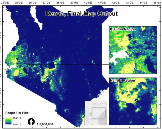
Final end-user 2010, 2015 and 2020 population data sets were generated for each country with an example of the final 2010 output for Kenya shown inFig. 2(please find Cambodia, Vietnam, and Kenya metadata reports and population maps attached asS1 File). We also produced ad-justed maps that match UN national total population estimates for each year according to the methodology described by Linard, et al. [17]. All maps have a spatial resolution set at 8.33 x 10⁻⁴degrees latitude/longitude and represent the number of people per grid cell.
Fig 2. The final redistributed population map for the Kenyan 1999 census data. Both census counts and the Random Forest predicted weighting layer for dasymetric redistribution were based on the finest level administrative units (Level 4) where a complete, country-wide coverage was available. doi:10.1371/journal.pone.0107042.g002
Random Forest Output
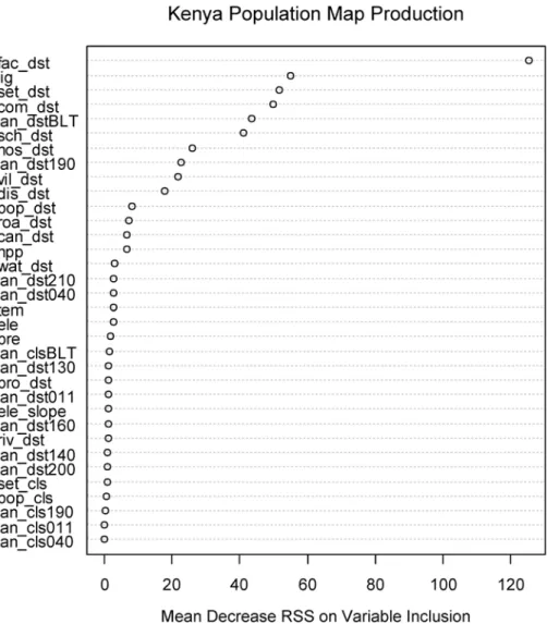
The Random Forest model performs substantially better than several other commonly used, freely available approaches for dasymetric mapping at country-level scales. An assessment of which of the ancillary data covariates are important for accurately estimating population densi-ty at the census unit level is produced by the Random Forest algorithm (see the third figure in each metadata report attached asS1 File). During the variable selection phase of the algorithm, the values of variable importance may fluctuate as the number of covariates is reduced. Howev-er, the relative ranking is quite stable among the top covariates. For Kenya, distance to health facility is by far the most important predictor (Fig. 3) for reducing the amount of variability left in the log population densities of the training census data. This indicates that this ancillary dataset is extremely valuable, even more than the distance-to-built land cover which is typically
Fig 3. Variable importance for Random Forest regression, presented as the mean decrease in residual sum of squares when the variable is included in a tree split. The model including variables here was used to produce the density weighting layer for the dasymetrically distributed population map inFig. 2. Variable names are defined and described inTable 1.
extremely important (see metadata reports inS1 File). This is likely due to the comprehensive and detailed nature of the health facility dataset [44].
Accuracy Assessments
The accuracies of the population maps which were constructed using coarser scale administra-tive units are presented inFig. 4and inTable 2. For Cambodia (Fig. 4a) there appears to be very little bias in prediction error across the range of observed census values. The calculated RMSE, % RMSE and MAE indicate that the performance of the new method is better than any of the other tested approaches (Table 2). Though not as tight as the relationship for Cambodia (Fig. 4a), the observed vs. predicted plot for Vietnam (Fig. 4b) shows that the RF methodology is not particularly biased for observed values larger than zero. Where observed census counts
Fig 4. Observed census counts plotted from the finer census administrative units versus the summed grid cell values from the population map estimated using coarser administrative units for a) Cambodia, b) Vietnam, and c) Kenya. Dotted lines in each figure represent the 1:1 line and prediction error is stated for each country by the RMSE, %RMSE and MAE values.
are zero, however, the methodology will predict a range of values, which indicates there may still be some refinement possible to better predict when census units include low or
zero counts.
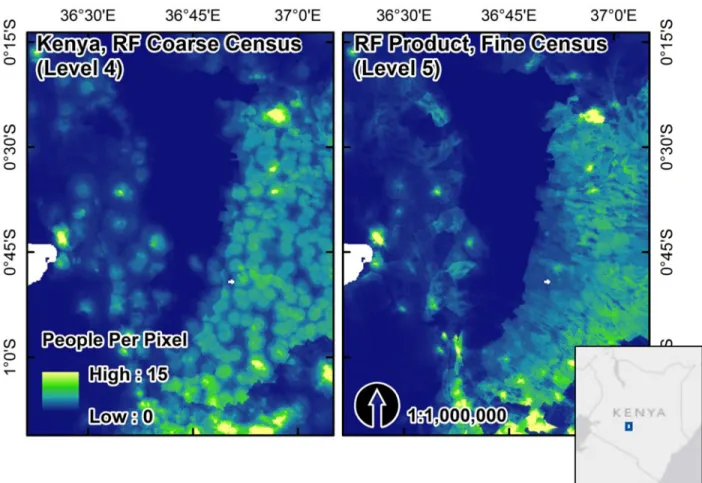
The use of finer-level administrative units in the algorithm increases the ability of the RF model to predict population density at smaller scales, which takes better advantage of useful ancillary datasets due to the increased variability explained in observed population counts. We show this visually by estimating the RF model and generating population maps for Kenya using finer level census units (Administrative Level 5, or‘sublocation’). These finer scale results show a smoother, more continuous redistribution of population versus the model estimated with coarser level administrative units (Administrative Level 4) (Fig. 5).
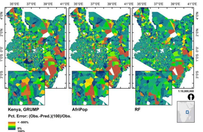
For validation purposes, we used the predicted population maps from Kenya estimated with the Level 4 administrative unit census data, and compared the percent residual, (observed— predicted) / observed) x 100) for each census unit summed within the admin Level 5 (finer scale) units (Fig. 6). A negative percent residual represents an over prediction, while the scale is bounded by 100% for the case where you predict zero but there were actually people counted within that census unit. The distribution of percent residuals shows that the RF approach re-sults in fewer extreme prediction errors across the entire country. Furthermore, there are fewer extremes in both large and small census units, indicating that the percent error is relatively consistent for both large and small population counts.
Discussion
Main Summary
The population mapping method presented here creates a dasymetric weighting scheme using an iterative Random Forest (RF) model with multiple ancillary data sources. By using this flexi-ble weighting algorithm we improve upon existing, freely availaflexi-ble population mapping ap-proaches and increase our ability to provide updated population maps for countries with census and ancillary data at spatial scales relevant to country-level population density maps. We compared this approach to other population map production algorithms. The AfriPop and AsiaPop approaches use a weighting scheme calculated from class-based combinations of land
Table 2. Accuracy assessment results for the RF, Afri/AsiaPop, GRUMP and GPW modeling methods for Cambodia, Vietnam and Kenya.
Country Method RMSE % RMSE MAE
Cambodia RF 3209.40 38.84 2026.73 AsiaPop 3834.51 46.40 2494.32 GRUMP 6767.39 81.89 3889.39 GPW 6794.88 82.22 4021.41 Vietnam RF 4367.00 61.96 2778.80 AsiaPop 4943.31 70.13 3007.04 GRUMP 6523.77 92.56 3771.64 GPW 7081.76 100.47 3844.47 Kenya RF 3956.74 91.36 1685.82 AsiaPop 5208.79 120.28 2184.64 GRUMP 6294.61 145.35 2383.64 GPW 6327.80 146.11 2304.70
Two different error assessment methods are presented: root mean square error (RMSE), also expressed as a percentage of the mean population size of the administrative level (% RMSE); and the mean absolute error (MAE).
cover, urban/rural built area delineation and climate zone information [17,19]. By incorporat-ing such information into the AfriPop/AsiaPop weightincorporat-ing methodology, census counts are dis-tributed more densely in human-modified areas than GRUMP and GPW, thereby increasing the accuracy of final the products (Fig. 7). The RF methodology we outline here improves upon this weighting algorithm by incorporating data sets other than just land cover and climate zone, including distance- to health facilities, schools, roads and many other features that may be good predictors or proxies for human population presence (Table 1). By including these fea-tures in the updated RF weighting algorithms we create population maps that are not only more accurate than GPW, GRUMP and AfriPop/AsiaPop (Table 2), but also represent variabil-ity in population densvariabil-ity as it relates to multiple biophysical and social features across
the landscape.
Methodology Considerations
One of the strengths of the Random Forest algorithm is the ability to incorporate many covari-ates with a minimum of tuning and supervision. These covariate data sets include night-time lights (e.g. Suomi NPP Visible Infrared Imaging Radiometer Suite (VIIRS)-derived data), to-pography (e.g. USGS SRTM-derived HydroSheds, ASTER DEM products), land cover (e.g. Landsat-derived classified data sets) and climatic information (e.g. WorldClim). A broad range
Fig 5. A visual comparison of Kenyan population maps for census data in 1999 produced at coarser administrative unit (Level 4) and finer-scale administrative unit (Level 5). The difference illustrates the finer gradations of RF model predictions for the density weighting layer when there are larger ranges of observed population densities present in training data (N = 505 for Level 4, N = 6622 for Level 5).
of country-specific data may also be incorporated to further refine any modeling effort. These data may include road and river networks, population center and building locations, protected area boundaries, and demography, among others. The primary challenge presented by combin-ing these disparate data in any modelcombin-ing effort lies in the multiple scales of measurement, often high correlation among data sets, the presence of highly nonlinear interactions and a mix of continuous and discrete distributional characteristics.
The Random Forest model estimated for Kenya (Fig. 4c) exhibits a slight tendency to over-predict at low population values and exhibits a wider spread around the 1:1 line. However, be-cause Kenya has a much larger range of census values with many smaller administrative units it exhibits the lowest MAE among the case study countries but the highest % RMSE. It remains a difficult country for which to predict population distributions at a very fine scale. But because the available census data are so fine, the dasymetric mapping approach for the final end-user product will still have high accuracy as the census counts“anchor” the end-user product pre-dictions to observed values at a smaller spatial scale than for many other countries. This “an-chor” effect minimizes the bias introduced by the “Ecological Fallacy” of using a model estimated with aggregated data, in this case the census unit, to predict at a much finer spatial scale. By redistributing population data within each census unit to predicted population densi-ty, estimates are guaranteed to at least be accurate when aggregated back to the census
unit level.
Fig 6. For Kenya we compared the summed predictions of population maps estimated using coarse census data (Level 4,“Division” level) to population counts at Level 5 (finer scale) units. We present prediction errors (observed minus predicted) as percentage values of the observed Level 5 census counts. The RF approach results in far fewer census units with extreme over predictions (negative percent residuals in yellows and oranges) and under predictions (positive percent residuals in dark blues).
Context
When developing models that incorporate multiple data sources there are two primary ap-proaches. The first relies on statistical models for predicting population density directly from multiple covariates [26]. These are often used at small geographic scales (sub-regional, metro-politan or county-level) and rely on highly detailed population count or density information for model estimation and often place restrictive demands on distributional requirements and assumptions. The second relies on creating a population redistribution weighting scheme that is combined with areal census counts, and with a dasymetric approach, spreads those counts across the area they represent as a function of the weights within each census area. This ap-proach can be used at large scales (i.e. country and continent scale) and can vary widely in the sophistication of the weighting scheme used. The most well-known large-scale projects using ancillary data sources are LandScan [13], AfriPop [5,17] and AsiaPop [19].
We are challenged to incorporate the vast and increasing amounts of spatial data being reg-ularly produced on features that influence population distributions (e.g. more detailed and ac-curate road locations, settlement centroids, building delineations). To take advantage of these data a flexible modeling approach capable of dealing with collinearity and nonlinearity in vari-able associations is required. The outlined RF methodology is highly resistant to over-fitting training data, exhibits a good balance of bias-variance optimization and generates estimates of both variable importance and model uncertainty as a byproduct of the cross-validation inher-ent to the fitting process [28,29]. Though in other applications it performs slightly worse than recent gradient boosting algorithms [45] the RF algorithm has fewer tuning parameters which makes it preferable in the semi-automated map production process we have developed here. Enabling a more semi-automated mapping approach is preferred here for generating cross-na-tional population surfaces with minimal country-specific tuning, thus providing updated pop-ulation data sets in a more timely and effective manner.
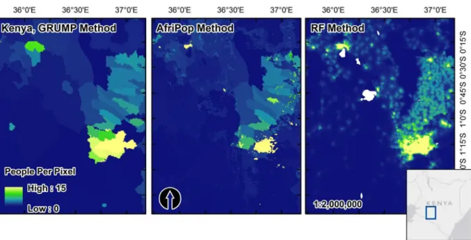
Fig 7. Visual comparisons of GRUMP, AfriPop and the RF-based population map from this study. Though this region northwest of Nairobi, Kenya is not a highly populated region this figure shows the results of the more detailed RF weighting layer versus the use of just urban areas (GRUMP) and land cover plus urban areas (AfriPop). The distinct edges in estimated people per pixel between census units are almost eliminated by the RF approach and it achieves greater consistency in predicted population density after census count redistribution.
Several features of the RF algorithm and their implications for the population distribution weighting layer warrant additional discussion. We use the natural log of the observed, census unit population densities as the response variable for RF model estimation. We found that by transforming the response variable prior to RF model fitting we consistently achieved higher prediction accuracies in the validation process we describe (Fig. 1,Table 2). Transformation of the covariates will not affect the explanatory power or fitting process of the RF algorithm [28] because splitting criteria at each node are evaluated along the entire range of bagged covariates. Therefore, any transformation of a covariate that does not affect the covariate’s rank order will not have an overall effect on model fitting or predictions. However, transformations of the re-sponse variable can have a significant impact on model fitting and performance because the range and features of the response distribution affect the values calculated for the splitting cri-teria objective function (sum of squared deviations for predictions in the RF regression case).
We evaluated several different transformations of the observed census-unit population den-sity including square root, log10, and others. The natural log transformation resulted in the
largest increases in prediction accuracy but have the consequence of requiring the removal of census-units with zero population densities from the training data prior to fitting. The gains are likely seen from the decreased impacts of prediction errors for large observed population densities, thus prioritizing prediction accuracy for lower- and mid-range population density areas. But predicting log-population density and back-transforming results in a dasymetric density weighting layer that has no cells with zeroes. This means that at least a small fraction of census population numbers will be spread to every cell of the resulting population map, except for those cells classified as water or missing in the land cover layer for which we define popula-tion density to be zero, or for areas that are outside the census unit boundaries. This may have implications for certain applications of the population maps where whole counts are preferred, however, statistical or spatial reassignment on a cell-by-cell basis could be performed by the end-user to alleviate this issue. Alternatives to the natural log transformation will be explored in future algorithm development to allow for zero population predictions and further refine-ment of the prediction accuracy. These could include a two-stage modeling approach, predict-ing zero or non-zero first and followpredict-ing up with the algorithm as we describe here for areas with predicted non-zero population density.
Another feature of the RF algorithm for regression that has implications for population maps and dasymetric weighting is that RF regression predictions are limited to the range of val-ues present in the training observations. Therefore, no extrapolation beyond the bounds of the population densities observed in the original training data is possible. Within the census-unit level we know that population density may be spatially heterogeneous, especially as census-unit sizes increase, but even within small census census-unit areas. Our primary assumption is that RF predictions at the pixel level, even limited to the range of observed population densities at the census-unit level, will accurately represent the spatial heterogeneity within the census-unit for more accurate dasymetric redistribution of population counts. This assumption is more likely to be true as you decrease the size of the census units with which the RF model is estimated, re-sulting in finer gradations of model predictions across the ranges of covariates used (Fig. 5). Fortunately, for countries with coarse census data (large census units relative to the country size and population density within them) the RF model will degrade gracefully to predictions of mean population density and bias in predictions will tend to be minimized in favor of less specificity. In other words the RF algorithm will do no worse than model approaches with less ancillary data.
However, the RF approach we outline here also offers a potential solution to the coarse cen-sus data problem. The demonstrated strength of the RF algorithm for countries with fine-scale census data, like those presented here, can be leveraged for those countries with coarser data.
By combining the forests produced from one or more countries with similar constraints on population distributions and available ancillary data, we can use the combined model to create a predicted density weighting layer for countries that have coarse census data. Furthermore, as more census data become available for single or multiple countries within a region, we can fur-ther refine RF predictions by sampling from and combining trees and forests which may yield better prediction accuracies than using a single RF model parameterized using coarse-scale census data.
Despite these caveats and considerations, the application of the Random Forest algorithm allows for increased detail in the final population redistribution, minimizing artifacts in the final population dataset. Data sets are more accurate than other large-scale regional and global scale population data sets (Table 2) and produce smoother, more continuous and‘realistic’ looking surfaces as a product of the increased amount of ancillary data used in the model pro-cess [26]. Variability at finer scales is an important consideration that the RF methodology in-corporates by using a significant number of ancillary datasets that inform the final population redistribution process for each country. We show that these ancillary datasets, collected region-ally and per-country may be incorporated into our flexible modeling framework more easily than with other approaches and allow us to quickly produce finer-scale, mapped population distribution products than previously available.
Conclusions
We present a semi-automated, dasymetric model for mapping human population distribution that provides a timely resource used for measuring impacts of population growth. Increased ac-curacy of projected changes in population patterns is important for policy and planning initia-tives at regional to global scales and results from this study provide a methodology for
generating highly accurate national-scale distributions of population data. By using a Random Forest algorithm to determine population density weightings, the model algorithm is more flexible in handling multiple covariates of both a discrete and continuous nature. The general methodology increases the sophistication of the weighting scheme first introduced in the Afri-Pop and AsiaAfri-Pop dasymetric mapping projects [5,17–19] by introducing a suite of ancillary datasets that enable finer-scale variability in population redistribution. Population datasets for 2010, 2015, and2020are freely available for download from the WorldPop Project (http://www. worldpop.org.uk/).
Supporting Information
S1 File. Population Maps, Metadata Reports and KML Files.For each country we produce population maps for the year the census data were collected (e.g.Fig. 5). In addition, popula-tion maps are adjusted to match UN estimates of growth for rural and urban areas to produce estimated population maps for 2010 and 2015. These estimates are also adjusted to match UN total population estimates for each country. The methodology for making these adjustments is detailed by Linard et al. [17]. In addition to the population maps themselves, the algorithm self-documents by creating a metadata report. This report includes not only information on the covariates included in each country’s model but also the Random Forest fitting informa-tion. Last, the population map for the census data year is tiled and saved into a Google Earth KML/KMZ file for easy overlay on top of high-resolution imagery. Examples of the metadata reports and KMZ files are attached with this manuscript as for Cambodia (KHM), Vietnam (VNM) and Kenya (KEN).
S2 File. Technical Fitting Details of the Random Forest Algorithm and Source Code. Though the randomForest package [29] provides the functionality to fit a model with an arbi-trarily large number of covariates and observations (limited only by memory and disk space) a limiting feature of our approach is the time spent during the prediction phase. During testing with covariates from Kenya we found that decreasing the number of predictors from 44 to 16 during the final forest growing stage and using the reduced forest for prediction over millions of pixels can result in time reduction of 1–2% per predictor decreased. For a prediction running in parallel, with a country the size of Kenya, on a standard dual core laptop or desktop proces-sor running at 2.5 GHz this can reduce prediction times by as much as five hours. This increase in efficiency comes with little to no trade-off in out-of-bag prediction accuracy. In practice model estimates are performed on a multi-core machine and run in parallel fashion over more than two cores, with the entire process running from data pre-processing to completion on the order of hours to as much as a day for very large countries. The data reduction method is at-tached, packaged as an R code snippet with included data and covariates shapefile to reproduce the method described. In the attached source code please assume that y_data is a vector con-taining log transformed population densities for each census unit in the data set. Also assume that x_data is a data.frame containing a row for each census unit and columns for each aggre-gated covariate (continuous measurements like distances or proportions are averaged, while categorical covariates are mode aggregated). The sample shapefile provided includes covariate data aggregated for Cambodia and the compressed R data frame files (for x_data and y_data) used with the included code snippet will recreate the Random Forest model estimation used for the final Cambodia maps presented in the paper are attached. All of the initial tuning parame-ters are estimated as a simple function of number of observed census units, while the tuneRF() function is used to find the optimal number of covariates to randomly select on at each branch point. These Random Forest objects are then used in a parallel fashion to generate per-pixel predictions of population density. These per-pixel predictions make up the layer used to dasy-metrically distribute census-level population counts.
(ZIP)
S3 File. Additional Accuracy Test Using Total Country-wide Population Redistribution. We illustrate the utility of the Random Forest methodology and the prediction density layer it produces by summing all census units into a single country-wide population count. We then distribute the total population number according to the relative weight for each pixel in our prediction layer, just as we would for individual census units. Doing this for Cambodia (S3 File) and comparing the distribution to results where individual census unit counts were used as the units for dasymetric redistribution (Fig. 4a) illustrates the utility of the prediction layer as a whole. The results show that though we lose some predictive power (illustrated by the greater spread around the 1:1 line) we are not increasing bias in our estimates (illustrated by the linear trend of the observed vs. predicted values along the 1:1 line). The resulting RMSE of 4672 indicates that even when eliminating the“anchor” effect of distributing census unit counts, the Random Forest methodology still outperformed the approaches used by GRUMP and GPW methods, even though they are both using finer-level census data to anchor their predictions.
(TIF)
Acknowledgments
We would like to thank the reviewers of this paper and the editors at PLOS One for their hard work and excellent feedback. This paper forms part of the output of the WorldPop Project
(http://www.worldpop.org.uk/) where a full list of data, funding and acknowledgements may be found.
Author Contributions
Analyzed the data: FRS AEG AJT. Contributed reagents/materials/analysis tools: FRS AEG CL AJT. Wrote the paper: FRS AEG CL AJT.
References
1. Balk DL, Deichmann U, Yetman G, Pozzi F, Hay SI, Nelson A. Determining global population distribu-tion: methods, applications and data. Adv Parasitol. 2006 [cited 2012 Nov 7]. 62:119–56. Available:
http://www.pubmedcentral.nih.gov/articlerender.fcgi?artid=3154651&tool = pmcentrez&rendertype = abstractPMID:16647969
2. Tatem AJ, Adamo S, Bharti N, Burgert CR, Castro M, Dorelien A, et al. Mapping populations at risk: im-proving spatial demographic data for infectious disease modeling and metric derivation. Popul Health Metr. 2012 [cited 2013 May 17]. 10(1):8. Available:http://www.pophealthmetrics.com/Content/10/1/8
doi:10.1186/1478-7954-10-8PMID:22591595
3. Salvatore M, Pozzi F, Ataman E, Huddleston B, Bloise M. Mapping global urban and rural population distributions [Internet]. Rome, Italy: Food and Agriculture Organization of the United Nations; 2005 [cited 2013 May 17]. Available:http://www.fao.org/docrep/009/a0310e/a0310e00.htm
4. United Nations. World Urbanization Prospects—The 2012 Revision. New York, NY; 2012. doi:10. 2149/tmh.2011-S05PMID:22500131
5. Tatem AJ, Noor AM, von Hagen C, Di Gregorio A, Hay SI. High resolution population maps for low in-come nations: combining land cover and census in East Africa. PLoS One. 2007 [cited 2012 Oct 31]. 2 (12):e1298. Available:http://www.pubmedcentral.nih.gov/articlerender.fcgi?artid=2110897&tool = pmcentrez&rendertype = abstractPMID:18074022
6. Gallego FJ, Batista F, Rocha C, Mubareka S. Disaggregating population density of the European Union with CORINE land cover. International Journal of Geographical Information Science. 2011. p. 2051–69. 7. Tatem AJ, Linard C. Population mapping of poor countries. Nature. Nature Publishing Group, a division of Macmillan Publishers Limited. All Rights Reserved.; 2011 [cited 2013 Jan 20]. 474(7349):36. Avail-able:http://dx.doi.org/10.1038/474036ddoi:10.1038/474036bPMID:21637245
8. Tobler W, Deichmann U, Gottsegen J, Maloy K. The Global Demography Project (Technical Report TR-95–6). Santa Barbara, CA: National Center for Geographic Information and Analysis, Department of Geography, University of California Santa Barbara; 1995.
9. Wu S, Qiu X, Wang L. Population Estimation Methods in GIS and Remote Sensing: A Review. GIScience Remote Sens. 2005 [cited 2013 Jan 10]. 42(1):80–96. Available:http://bellwether. metapress.com/openurl.asp?genre = article&id = doi:10.2747/1548–1603.42.1.80
10. Balk DL, Yetman G. The Global Distribution of Population: Evaluating the gains in resolution refinement [Internet]. New York, NY: Center for International Earth Science Information Network (CIESIN); 2004. Available:http://sedac.ciesin.org/gpw/docs/gpw3_documentation_final.pdf
11. Balk DL, Pozzi F, Yetman G, Deichmann U, Nelson A. The distribution of people and the dimension of place methodologies to improve the global estimation. Urban Remote Sensing Conference [Internet]. New York, NY: The World Bank; 2005. p. 1–6. Available:http://sedac.ciesin.columbia.edu/gpw/docs/ UR_paper_webdraft1.pdf
12. Bhaduri B, Bright E, Coleman PR, Urban ML. LandScan USA: a high-resolution geospatial and tempo-ral modeling approach for population distribution and dynamics—Tags: CENSUS POPULATION. Geo-Journal. 2007. 69(1/2):103–17. Available:http://connection.ebscohost.com/c/articles/27560012/ landscan-usa-high-resolution-geospatial-temporal-modeling-approach-population-distribution-dynamics
13. Dobson JE, Brlght EA, Coleman PR, Worley BA. LandScan: A Global Population Database for Estimat-ing Populations at Risk. Photogramm Eng Remote Sens. 2000. 66(7):849–57.
14. CIAT. Latin American and Caribbean Population Distribution Database, Version 3 [Internet]. Centro Internacional de Agricultura Tropical (CIAT). 2005 [cited 2013 Apr 8]. Available:http://gisweb.ciat.cgiar. org/population/dataset.htm
15. Nelson A. African Population Database Documentation [Internet]. Center for International Earth Sci-ence Information Network (CIESIN), Columbia University. 2004 [cited 2013 Apr 8]. Available:http://na. unep.net/siouxfalls/globalpop/africa/Africa_index.html
16. Deichmann U. A Review of Spatial Population Database Design and Modeling [Internet]. Santa Bar-bara, CA: National Center for Geographic Information and Analysis; 1996. Available:http://www.ncgia. ucsb.edu/Publications/Tech_Reports/96/96–3.PDF
17. Linard C, Gilbert M, Snow RW, Noor AM, Tatem AJ. Population distribution, settlement patterns and ac-cessibility across Africa in 2010. PLoS One. 2012 [cited 2012 Dec 29]. 7(2):e31743. Available:http:// www.pubmedcentral.nih.gov/articlerender.fcgi?artid=3283664&tool = pmcentrez&rendertype = abstract
18. Linard C, Tatem AJ. Large-scale spatial population databases in infectious disease research. Int J Health Geogr. 2012 [cited 2013 Jan 10]. 11:7. Available:http://www.pubmedcentral.nih.gov/ articlerender.fcgi?artid=3331802&tool = pmcentrez&rendertype = abstractdoi: 10.1186/1476-072X-11-7PMID:22433126
19. Gaughan AE, Stevens FR, Linard C, Jia P, Tatem AJ. High Resolution Population Distribution Maps for Southeast Asia in 2010 and 2015. Pappalardo F, editor. PLoS One. 2013 [cited 2013 Feb 14]. 8(2): e55882. Available:http://dx.plos.org/10.1371/journal.pone.0055882doi:10.1371/journal.pone. 0055882PMID:23418469
20. Anderson DE, Anderson PN. Population estimates by humans and machines. Photogramm Eng. 1973 [cited 2013 Jan 20]. 39(2):147–54. Available:http://trid.trb.org/view.aspx?id=92581
21. Lo CP. Automated population and dwelling unit estimation from high-resolution satellite images: a GIS approach. Int J Remote Sens. Taylor & Francis; 1995 [cited 2013 Jan 20]. 16(1):17–34. Available:
http://dx.doi.org/10.1080/01431169508954369
22. Sutton P, Roberts D, Elvidge C, Baugh K. Census from Heaven: An estimate of the global human popu-lation using night-time satellite imagery. Int J Remote Sens. Taylor & Francis; 2001 [cited 2012 Dec 19]. 22(16):3061–76. Available:http://www.tandfonline.com/doi/abs/10.1080/01431160010007015
23. Azar D, Graesser J, Engstrom R, Comenetz J, Leddy RM, Schechtman NG, et al. Spatial refinement of census population distribution using remotely sensed estimates of impervious surfaces in Haiti. Int J Remote Sens. 2010 [cited 2013 Jan 9]. 31(21):5635–55. Available:http://www.tandfonline.com/doi/ abs/10.1080/01431161.2010.496799
24. Chen K. An approach to linking remotely sensed data and areal census data. Int J Remote Sens. 2002 [cited 2012 Dec 25]. 23(1):37–48. Available:http://www.tandfonline.com/doi/abs/10.1080/
01431160010014297
25. Linard C, Gilbert M, Tatem AJ. Assessing the use of global land cover data for guiding large area popu-lation distribution modelling. GeoJournal. 2010 [cited 2012 Dec 7]. 76(5):525–38. Available:http://www. springerlink.com/index/10.1007/s10708–010–9364–8PMID:23576839
26. Azar D, Engstrom R, Graesser J, Comenetz J. Generation of fine-scale population layers using multi-resolution satellite imagery and geospatial data. Remote Sens Environ. 2013 [cited 2013 Jan 10]. 130:219–32. Available:http://linkinghub.elsevier.com/retrieve/pii/S0034425712004543
27. Lung T, Lübker T, Ngochoch JK, Schaab G. Human population distribution modelling at regional level using very high resolution satellite imagery. Appl Geogr. 2013 [cited 2013 May 3]. 41:36–45. Available:
http://dx.doi.org/10.1016/j.apgeog.2013.03.002
28. Breiman L. Random Forests. Mach Learn. 2001 [cited 2013 Jan 24]. 45(1):5–32. Available:http://link. springer.com/article/10.1023/A:1010933404324
29. Liaw A, Wiener M. Classification and Regression by randomForest. R News. 2002. 2(3):18–22. Avail-able:http://cran.r-project.org/doc/Rnews/
30. MDA Federal Inc. EarthSat GeoCover LC Overview [Internet]. 2007. Available:http://www.mdafederal. com/geocover/geocoverlc/gclcoverview
31. Lehner B, Verdin K, Jarvis A, Fund WW. HydroSHEDS Technical Documentation [Internet]. World Wild-life Fund; 2006 p. 27. Available:http://www.worldwildlife.org/freshwater/pubs/HydroSHEDS_TechDoc_ v10.pdf
32. Running SW, Nemani RR, Heinsch FA, Zhao M, Reeves M, Hashimoto H. A Continuous Satellite-De-rived Measure of Global Terrestrial Primary Production. Bioscience. 2004 [cited 2013 Mar 5]. 54 (6):547. Available:http://www.jstor.org/stable/10.1641/0006–3568(2004)054[0547:ACSMOG]2.0.CO;2 33. NOAA. VIIRS Nighttime Lights—2012 [Internet]. Earth Observation Group, National Geophysical Data
Center, National Oceanic and Atmospheric Administration (NOAA). 2012 [cited 2013 Apr 8]. Available:
http://www.ngdc.noaa.gov/dmsp/data/viirs_fire/viirs_html/viirs_ntl.html
34. Hijmans RJ, Cameron SE, Parra JL, Jones PG, Jarvis A. Very high resolution interpolated climate sur-faces for global land areas. Int J Climatol. 2005 [cited 2013 Mar 3]. 25(15):1965–78. Available:http:// doi.wiley.com/10.1002/joc.1276
35. NGA. Vector Map (VMap) Level 0 [Internet]. National Geospatial-Intelligence Agency (NGA). 2005. Available:http://geoengine.nga.mil/geospatial/SW_TOOLS/NIMAMUSE/webinter/rast_roam.html
36. ESRI. ArcGIS Desktop Release 10.0. Redlands, CA: Environmental Systems Research Institute; 2011.
37. Schneider A, Friedl MA, Potere D. A new map of global urban extent from MODIS satellite data. Environ Res Lett. 2009 [cited 2012 Nov 5]. 4(4):044003. Available:http://stacks.iop.org/1748–9326/4/i=4/a= 044003?key = crossref.6bde1987a5db9cd29ac85e4c73503481
38. Schneider A, Friedl MA, Potere D. Mapping global urban areas using MODIS 500-m data: New meth-ods and datasets based on“urban ecoregions.” Remote Sens Environ. 2010 [cited 2012 Nov 8]. 114 (8):1733–46. Available:http://linkinghub.elsevier.com/retrieve/pii/S003442571000091X
39. OSM. OpenStreetMap Base Data [Internet]. OpenStreetMap.org. 2013. Available:http://www. openstreetmap.org/
40. Tatem AJ, Noor AM, Hay SI. Assessing the accuracy of satellite derived global and national urban maps in Kenya. Remote Sens Environ. 2005 [cited 2013 Feb 12]. 96(1):87–97. Available:http://www. pubmedcentral.nih.gov/articlerender.fcgi?artid=3350068&tool = pmcentrez&rendertype = abstract
PMID:22581985
41. Breiman L. Bagging Predictors. Mach Learn. 1996. 24(2):123–40. PMID:8725661
42. Sikonja MR-. Improving Random Forests. In: Boulicaut JF, editor. Machine Learning, ECML 2004 Pro-ceedings. Berlin, Germany: Springer; 2004.
43. R Core Team. R: A Language and Environment for Statistical Computing [Internet]. Vienna, Austria; 2013 [cited 2013 May 24]. Available:http://www.r-project.org/doi:10.3758/s13428-013-0330-5PMID:
23519455
44. Noor AM, Alegana VA, Gething PW, Snow RW. A spatial national health facility database for public health sector planning in Kenya in 2008. Int J Health Geogr. 2009 [cited 2013 Apr 8]. 8:13. Available:
http://www.pubmedcentral.nih.gov/articlerender.fcgi?artid=2666649&tool = pmcentrez&rendertype = abstractdoi:10.1186/1476-072X-8-13PMID:19267903
45. Hastie T, Tibshirani R, Friedman J. The Elements of Statistical Learning: Data Mining, Inference, and Prediction, Second Edition (Springer Series in Statistics) [Internet]. Springer; 2009 [cited 2013 Jan 11]. Available:http://www.amazon.com/The-Elements-Statistical-Learning-Prediction/dp/0387848576doi:
10.1016/j.neunet.2009.04.005PMID:19443179
46. Tatem AJ, Noor AM, Hay SI. Defining approaches to settlement mapping for public health management in Kenya using medium spatial resolution satellite imagery. Remote Sens Environ. 2004 [cited 2013 Feb 12]. 93(1–2):42–52. Available:http://www.pubmedcentral.nih.gov/articlerender.fcgi?artid= 3350067&tool = pmcentrez&rendertype = abstractPMID:22581984
47. IUCN and UNEP. The World Database on Protected Areas (WDPA) [Internet]. Cambridge, UK: UNEP-WCMC; 2012. Available:http://www.protectedplanet.net
48. HR-COD. Humanitarian Response [Internet]. Common and Fundamental Operational Datasets Regis-try. 2013 [cited 2013 May 24]. Available:http://cod.humanitarianresponse.info/country-region/ cambodia
49. Kenya Open Data. Open Kenya, Transparent Africa [Internet]. Kenya Primary Schools, 2007. 2013 [cited 2013 May 24]. Available: https://opendata.go.ke/Education/Kenya-Primary-Schools-2007/p452-xb7c