Research note on mapping allergenic tree species distributions in Belgium

(1)

RESEARCH OUTPUTS / RÉSULTATS DE RECHERCHE

Author(s) - Auteur(s) :

Publication date - Date de publication :

Permanent link - Permalien :

Rights / License - Licence de droit d’auteur :

Institutional Repository - Research Portal

Dépôt Institutionnel - Portail de la Recherche

researchportal.unamur.be

University of Namur

Research note on mapping allergenic tree species distributions in Belgium

Dujardin, Sebastien; Linard, Catherine; DENDONCKER, Nicolas

Publication date: 2017

Document Version

Publisher's PDF, also known as Version of record Link to publication

Citation for pulished version (HARVARD):

Dujardin, S, Linard, C & DENDONCKER, N 2017, Research note on mapping allergenic tree species distributions in Belgium.

General rights

Copyright and moral rights for the publications made accessible in the public portal are retained by the authors and/or other copyright owners and it is a condition of accessing publications that users recognise and abide by the legal requirements associated with these rights. • Users may download and print one copy of any publication from the public portal for the purpose of private study or research. • You may not further distribute the material or use it for any profit-making activity or commercial gain

• You may freely distribute the URL identifying the publication in the public portal ?

Take down policy

If you believe that this document breaches copyright please contact us providing details, and we will remove access to the work immediately and investigate your claim.

(2)

BRAIN-be

BELGIAN RESEARCH ACTION THROUGH INTERDISCIPLINARY NETWORKS

BR/154/A1/RespirIT

Research note on mapping allergenic tree species

in Belgium

14/04/2017

Updated on 26/02/2021

Dr. Sébastien Dujardin

Pr. Catherine Linard

Pr. Nicolas Dendoncker

(3)

1. Introduction

The BRAIN-be/RespirIT research project (contract number: BR/154/A1/RespirIT) aims at exploring and understanding the spatial and temporal effects of plant diversity on respiratory health. By linking the information on the whereabouts and medical condition of individuals to spatially explicit information of plant diversity, air quality and pollen concentrations, it has the ambition to quantitatively, dynamically, and spatially study plant diversity effects on allergic symptom severity. Yet, spatially explicit information on plant diversity is not readily available for Belgium and ready-made methods to link existing land cover maps to proxies of plant diversity are not available. Consequently, the work package 3 of the RespirIT research project seeks to provide spatially explicit proxies for plant diversity by (i) mapping the location of targeted allergenic tree species (task 3.1.1) and (ii) deriving spatially explicit proxies of plant diversity (task 3.1.2).

Within this research note, we report on the investigations accomplished to characterise our study area in terms of plant diversity. First, we provide an overview of the dataset inventory undertaken for mapping allergenic tree species in Belgium. We review the different types of datasets currently available and expose their thematic and spatial resolutions for characterising land use and plant diversity in Belgium. Second, we detail a method for mapping allergenic tree species at the national scale using datasets available within both the Flemish and the Walloon regions. Third, we expose and discuss our main results, including the presence or absence of allergenic trees across Belgium, the spatial distribution of three selected allergenic trees (Alnus, Betula, and Corylus), as well as their relative share in terms of basal area. Finally, we expose the key learnings honed through the mapping of allergenic tree species in Belgium and provide several research outlooks for future research.

2. Dataset inventory

Investigations started with a review of current database available in Belgium allowing for characterizing land use and vegetation cover. We identified three relevant types of georeferenced datasets for studying the spatial effects of plant diversity on respiratory health.

Firstly, several land use maps are available in both Flanders and Wallonia for describing land uses at a high spatial resolution. However, the Flemish and Walloon maps contain different categories of land use. This creates multiple matching issues when considering merging both datasets. Yet, the IGN

(5)

Secondly, no national-scale biodiversity map exists at this time of writing. While Flanders has completed a “biological valuation map”, Brussels and Wallonia are currently in the process of elaborating such a map. Detailed biodiversity inventories exist but need to be georeferenced and mapped. Nonetheless, a useful indicator covering the entire country is available from the LIFEWATCH project. A greenness indicator is available at a 1x1 km raster resolution to characterise plant phenology at high temporal resolution (i.e. across the weekly, monthly, yearly periods).

Thirdly, the most detailed and up-to-date information about tree diversity is contained within forest inventories. Both Flanders and Wallonia have undertaken a region-wide survey characterizing the type of tree species observed within forested areas. These datasets have a thematic resolution differentiating the tree selected allergenic tree species investigated within this research project: namely Alnus, Betula, and Corylus. These are available upon request by the « Agentschap voor Natuur en Bos » and the « Faculté universitaire des Sciences agronomiques de Gembloux » (Unité de Gestion des Ressources forestières et des Milieux naturels), respectively.

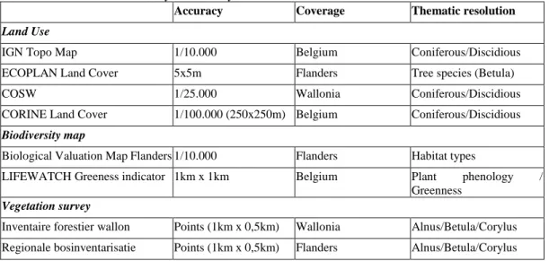
Table 1. Dataset inventory summary

Accuracy Coverage Thematic resolution

Land Use

IGN Topo Map 1/10.000 Belgium Coniferous/Discidious ECOPLAN Land Cover 5x5m Flanders Tree species (Betula) COSW 1/25.000 Wallonia Coniferous/Discidious CORINE Land Cover 1/100.000 (250x250m) Belgium Coniferous/Discidious

Biodiversity map

Biological Valuation Map Flanders 1/10.000 Flanders Habitat types

LIFEWATCH Greeness indicator 1km x 1km Belgium Plant phenology / Greenness

Vegetation survey

Inventaire forestier wallon Points (1km x 0,5km) Wallonia Alnus/Betula/Corylus Regionale bosinventarisatie Points (1km x 0,5km) Flanders Alnus/Betula/Corylus

3. Allergenic tree species distributions

3.1. Forest inventory data

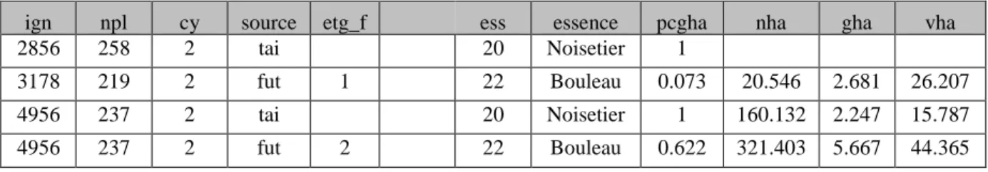
The most detailed and up-to-date information about tree abundance currently available in Belgium is contained within forest inventories. As shown in Error! Reference source not found., these dataset allow covering forested areas which represent 23% of the total land area in Belgium. Both Flanders (see Afdeling Bos & Groen ( 2001)): and Wallonia (see Rondeux and Lecomte, 2010, Alderweireld et al., 2015) have undertaken a region-wide survey characterizing the type of tree species observed within forested areas. These dataset have a thematic resolution that differentiates the selected

(6)

allergenic tree species investigated within this study, namely Alnus, Betula, and Corylus. We processed each forest inventory separately and then merged both dataset after having checked data consistency.

The main purpose of our analysis was to extract information from the Flemish and Walloon forest inventories about allergenic trees and provide an indicator of their relative abundance within a given tree stand. This was measured by calculating an overall percentage of basal area (i.e. the area of a given section of land that is occupied by the cross-section of tree trunks and stems at the base) for the selected allergenic trees (Alnus, Betula, and Corylus) per sampling plot. In practical terms, we first calculate a specific basal area (in m²/ha) of each allergenic trees species studied. Then, we compute the basal area of all trees observed within the plot. Finally, we calculate a final indicator, which is an overall relative percentage of basal area.

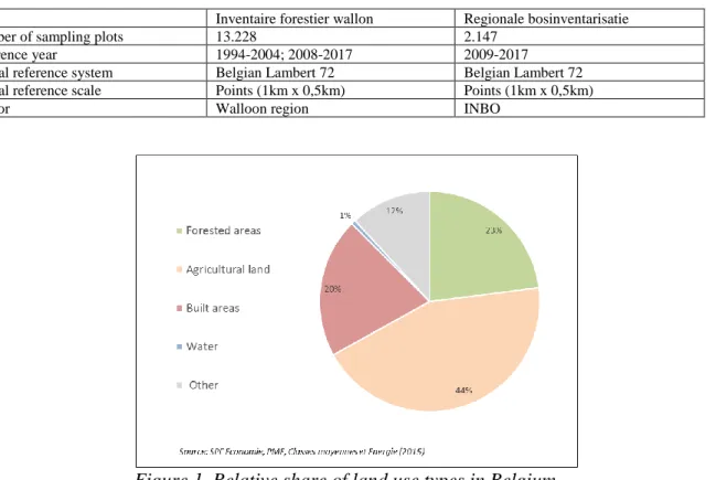
Table 2 Metadata of both forest inventories

Inventaire forestier wallon Regionale bosinventarisatie Number of sampling plots 13.228 2.147

Reference year 1994-2004; 2008-2017 2009-2017 Spatial reference system Belgian Lambert 72 Belgian Lambert 72 Spatial reference scale Points (1km x 0,5km) Points (1km x 0,5km)

Author Walloon region INBO

Figure 1. Relative share of land use types in Belgium

3.1.1. Processing the Walloon forest inventory dataset 3.1.1.1. Dataset’s content

(7)

cycles were undertaken. The first one took 14 years long. The second one started in 2008 and is still ongoing (to date, 50% is complete). The dataset contains two main tables.

The first table provided within the dataset (sheet “Placettes”) details the general characteristics of each plot, including:

- Plot’s geographic coordinates

- Date surveyed (ranging from May 2008 to March 2015) - Overall type of tree stand (e.g. oak grove, pine forest, etc.) - Structure (coppice, tree stand forest, etc.)

- The Waleunis code classification

A second table (sheet “Essence”) provides information about the allergenic tree species surveyed within the plot, namely alnus, betula and corylus (respectively alder, birch, and hazel in English). For a given plot, a new line is added each time a different type of tree is observed. Trees are differentiated on the basis of their structure which is either under the form of a coppice (taillis) or a stand forest (futaie). Stand forests are then sub-divided in two categories of level 1 and 2 (étage forestier).

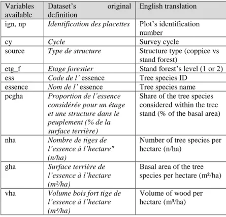
Within the sample table below for instance, the third line corresponds to a corylus observed under the form of a coppice. On the same plot (line four), betula is also observed under the form of a tree stand of level 2 (high trees).

Table 3. Dataset extract describing the type of trees observed

ign npl cy source etg_f ess essence pcgha nha gha vha

2856 258 2 tai 20 Noisetier 1

3178 219 2 fut 1 22 Bouleau 0.073 20.546 2.681 26.207

4956 237 2 tai 20 Noisetier 1 160.132 2.247 15.787

4956 237 2 fut 2 22 Bouleau 0.622 321.403 5.667 44.365

3.1.1.2. Variables available

The dataset “essence” contains different measures describing the presence of allergenic trees. Two of these are of particular interest for the purpose of this study: the type of tree observed (variable “ess” or “essence”) and the share of tree species within the tree stand (variable “pcgha”).

The variable “ess” allows identifying the type of allergenic tree observed within a plot. It has, however, some limitations as the count only includes trees with a circumference greater than 20 cm.

(8)

Besides, a threshold of minimum 20 trees has been set by surveyors for sampling corylus (see first line in table 1 above). From this limitation, the variables “nha”, “gha”, and “vha” are not calculated. The variable “pcgha” on the opposite is better suited for evaluating the relative presence of allergenic trees. When a tree with a circumference under 20 cm is observed within a plot, the species’ relative share within the tree stand is still provided based on an estimation from the surveyor.

Table 4. Variables description Variables

available

Dataset’s original definition

English translation ign, np Identification des placettes Plot’s identification

number

cy Cycle Survey cycle

source Type de structure Structure type (coppice vs stand forest)

etg_f Etage forestier Stand forest’s level (1 or 2) ess Code de l’ essence Tree species ID

essence Nom de l’ essence Tree species name pcgha Proportion de l’essence

considérée pour un étage et une structure dans le peuplement (% de la surface terrière)

Share of the tree species considered within the tree stand (% of the basal area)

nha Nombre de tiges de l’essence à l’hectare" (n/ha)

Number of tree species per hectare (n/ha)

gha Surface terrière de l’essence à l’hectare (m²/ha)

Basal area of the tree species per hectare (m²/ha) vha Volume bois fort tige de

l’essence à l’hectare (m³/ha)

Volume of wood per hectare (m³/ha)

Note that the first dataset (sheet “Placettes”) contains two entries with geographic coordinates defining the plot location: one is derived from the IGN cartographic grid (which serves as the reference for the sampling), while the other one contains the GPS coordinates from the field. We choose to use the GPS coordinates from the field in prior. When the latter was not available, we used the one from the sampling grid to locate the plot.

3.1.1.3. Aggregation procedures • Alnus incana vs Alnus glutinosa

(9)

The dataset differentiates the Alnus incana and the Alnus glutinosa. When those two types of tree are observed within the same plot, we aggregated these under the general tree category “Alnus” in order to simplify the analysis. In total, Alnus is observed within 169 plots. Among these plots, 139 plots contain alnus incana or alnus glutinosa only, but 30 plots contain a combination of both species. For these cases, all variables were summed up.

• Coppice vs tree stand

Likewise, when the same type of allergenic tree was observed under two different forms (e.g. under the form of coppice and high stand forest of level 1), we also summed the two observations into one observation only.

Consequently, these two aggregations simplify the dataset for 285 plots (19.6%) where details about the type of Alnus observed and/or the tree species’ structure (coppice, tree stand of level 1 or 2) are not available anymore.

3.1.1.4. Determination of predicted values for non-measured trees

The WFI contains an important number of non-measured trees whose circumference is lower than 20cm. As a result, the basal area in m²/ha is not provided for these observations (see first row in Table 1 for instance). In total, non-measured trees represent 36,7% of the dataset (690 observations). Yet, surveyors provided an estimated overall basal area in percent (variable “pcgha”) per tree species and tree structure. Drawing upon this information, we computed an estimated basal area in m²/ha using values from measured trees.

The approach undertaken was two-fold as we considered pure tree stands (pcgha =100%) separately from those containing another tree species (pcgha < 100%). Indeed, a coppice of corylus under a tree stand with of basal area of 50% has not the same meaning than a pure coppice of corylus with a basal area of 100%. The latter’s basal area (variable “gha” in m²/ha) may be higher than the former.

Therefore, for trees with a pcgha of 100%, we calculated an average gha per tree specie (Alnus, Betula, and Corylus) and structure (coppice vs tree stand). No values were calculated for corylus under the form of a tree stand as this type of tree structure does not exist. The following mean values (𝑥̅) were assigned:

(10)

Coppice Tree stand

N 𝑥̅ N 𝑥̅

Alnus 18 12.2 11 14.3 Betula 66 6.4 57 12.4 Corylus 13 2.6 NA NA

Then, for tree species with a pcgha lower than 100%, we built five linear regression models. By establishing a statistical relationship between measured gha and pcgha, we were able to predict and assign a gha value for non-measured observations. As the figure below shows, the correlation between these two variables vary depending on the observations available per tree species (k) and structure (l). The weakest relationship was found for coppices of corylus (plot C; R² = 0,513), while the strongest relationship was observed for Alnus under the form of a tree stand (plot D; R² = 0,842).

Predicted values were determined as follow:

gha_jk = pcgha_jk∗ E_jkl

With: ghajk = predicted basal area of tree specie k for plot j (m²/ha)

pcghajk = field-estimated basal area of non-measured tree species k (%) Ejkl = linear regression model estimate for tree specie k and strucure l (m²/ha)

(11)

Coppice Tree stand

Alnus

Betula

Corylus

In total, 1.880 observations from the initial dataset were trimmed down to 1.722 observations after aggregation (8,4% decrease). These 1.722 observations of allergenic trees are found within a total number of 832 sampling plots. When joined to the entire database from the Walloon forest inventory, plots containing at least one allergenic tree represent 7,5% of the dataset.

3.1.2. Processing the Flemish forest inventory dataset

3.1.2.1. Dataset input tables

The Flemish Forest Inventory (FFI) database was provided under the form of an access database. It contains more than 83 tables with information about tree structure, plot types, surveyors, etc. (see Wouters et al., 2008). One table named "Trees_2eBosinv" was selected and exported for processing in R. Table 4 shows an extract of this table, including 9 selected variables used for the purpose of this study. Within the sample table below for instance, the two first lines correspond to two Alnus trees

(12)

(Species “10”). On the same plot (line 3 and 4), two Betula are also observed (Species “12”). All trees are alive (status tree = 1).

Table 5. Dataset extract with selected variables

IDPlots X_m Y_m ID Species Perimet

er_cm Status_ tree Dumm yID_A 3 Dumm yID_A 3 157138 -4.936 -4.936 8 10 58 1 7 0 157138 0.257 0.257 1 10 30 1 1 0 157138 1.573 1.573 7 12 70 1 6 0 157138 2.887 2.887 6 12 30 1 5 0

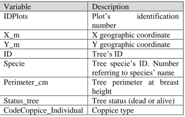
Table 5 provides a definition of the key variables used for evaluating trees’ basal area and mapping species’ spatial distribution.

Table 6.Variables description

Variable Description

IDPlots Plot’s identification

number

X_m X geographic coordinate

Y_m Y geographic coordinate

ID Tree’s ID

Specie Tree specie’s ID. Number

referring to species’ name Perimeter_cm Tree perimeter at breast

height

Status_tree Tree status (dead or alive) CodeCoppice_Individual Coppice type

3.1.2.2. Data managment and selection

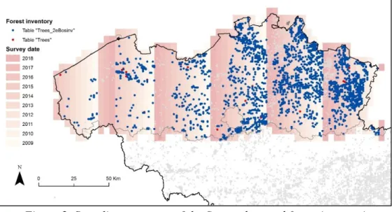
A comparison between the first and second forest inventories was made in order to identify the most relevant dataset to use. In this regard, the table "Trees" (considered as the 1st inventory) and the table "Trees_2eBosinv" (the 2nd forest inventory) were analysed compartively. The table "Trees_2eBosinv" is definitively the most comprehensive dataset. It contains 2.156 plots in total, while the table "Trees" contains 1.721 plots only. Besides, all plots (depite 24 exceptions) from the first inventory are found within the second one (see Figure 2 below). The survey grid (red tiles in Figure 2 or ‘rooster’ shapefile) allowed identifying areas were data are not up to date yet. These are plots where field surveys are planned for the year 2018 and 2017.

(13)

Figure 2. Sampling coverage of the first and second forest inventories

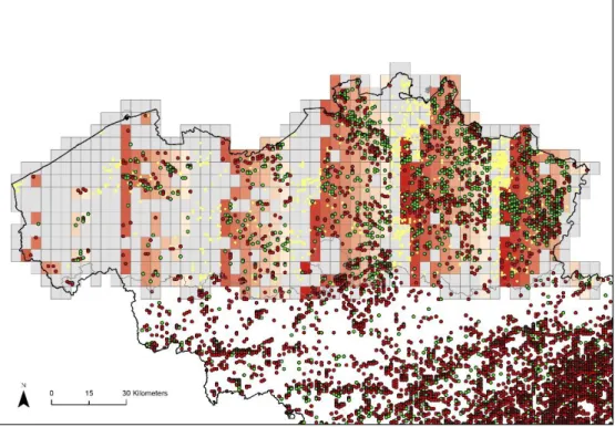
Such data spatial coverage gaps has to crarfully taken into account for the next modelling steps. In Error! Reference source not found.Figure 3 below, we illustrate these gaps by showing (i) the plots contained in the FFI database where, according to our calculations, there is either no allergenic tree (red points) or between 0% and 100% of the total basal area (green points). (ii) In yellow, the plots we expect to fall within a forested area (attirubte 'bos'=1 within the orignial ‘invb2’ shapefile that contains all the sampling plots). Their absence within the IFF dataset can be explained by the fact that either the plot does not exist anymore in the surey or has not been (re)surveyed yet, which explains why it is absent from the FFI database. (iii) The red rectangles consist of tiles from the ‘rooster’ shapefile (see Figure 3 above) that match with the plots extracted from the FFI database analysis. Finally, (iv) the grey rectangles are the tiles from the ‘rooster’ shapefile that do not match with the plots extracted from the FFI database analysis. Fortunately, since we received an updated version of the the Flemish forst inventory database in 2019, the yellow points and missing areas in grey are now included in the database and can be considered for predicting the distribution of allergenic tree species (see updated maps in the result sections).

(14)

Figure 3. Illustration of data spatial coverage gaps within the Flemish forest inventory.

The dataset selected contains 43.582 observations in total. The first step needed for processing this dataset is to remove all dead trees (2.611 observations) and keep living trees using the variable “Status_tree”. Then, a selection is operated to extract 3 allergenic tree species. This selection is based on the variable “species” (see table 6 below).

Table 7. List of allergenic tree species

Species Dataset’s original name Scientific name

10 Zwarte els Alnus glutinosa (L.) Gaertn.

11 Zwarte els Alnus incana (L.) Moench

1470* Hartbladige els* Alnus cordata (Loisel.) Duby*

12 Berk Betula tremula/alba

146* Zachte berk* Betula alba L.*

128* Ruwe berk* Betula pendula Roth*

14 Hazelaar Corylus avellana L.

*Not considered for analysis

The FFI contains three additional types of Betula compared to the WFF (species “1470”, “146”, and “128”). So far, these were not considered for the analysis in order to facilitate the comparison between datasets. Not considering these tree species means deleting 7 observations in total. This low number of Betula alba L. and Betula pendula Roth is due to the lack of specification of tree species by fieldworks who do not specify the type of species when surveying the plots.

(15)

Number of observations N Alnus incana 217 Alnus glutinosa 2251 Betula 4938 Corylus 419

3.1.2.3. Calculation of tree species’ basal area

Unlike the WFI, the FFI does not contain a variable describing trees’ basal area. Drawing upon Afdeling Bos & Groen ( 2001, p.29-30), we thus calculated a basal area according to the following third-step procedure.

First, a basal area for each individual tree within a plot is calculated following this equation:

With: gij = basal area of tree i wihtin the sampling plot j (m²)

cij = perimeter of tree i within the sampling plot j (cm), i.e. variable “Tree_perimeter”.

Second, a total basal area per hectare is calculated depending on the type of sampling plot (A2, A3 or A4).

With: Gjk = total basal area of allergenic trees k within the sampling plot j (m²/ha)

gijk = basal area of tree i within the sampling plot j (m²)

n2jk,n3jk,n4jk = number of trees k from plot type A2, A3, and A4 within plot j F2, F3, F4 = extension factor for plot type A2, A3, and A4

The extension factor used were:

- plot type A1: R1 = 2,25 m → F1 = 628,76 - plot type A2: R2 = 4,5 m → F2 = 157,19

(16)

- plot type A3: R3 = 9 m → F3 = 39,30 - plot type A4: R4 = 18 m → F4 = 9,82

Four plot types were identified using variables “perimter” and “Height” based on the following conditions detemrined by Afdeling Bos & Groen ( 2001, p.29-30):

- plot type A1: “zaailingen” with a total heigh < 2m

- plot type A2: Coppice; trees with perimeter < 22cm and a total height >= 2m - plot type A3: Trees with perimeter between 22cm and 122cm

- plot type A4: Tree with perimeter > 122cm

Third, after having calculated this basal area for allergenic tree species (Gjk), a second basal area (Gjf) is caclulated for all tree species observed within the samping plot.

Drawing upon these two values, a relative global basal area in percent is finally measured as follow:

𝐺𝑗 =Gjk

Gjf ∗ 100

With: Gj = relative basal area of allergenic trees k for plot j (%) Gjk = basal area of allergenic tree species (m²/ha)

(17)

3.1.3. Creating a Belgian forest inventory dataset

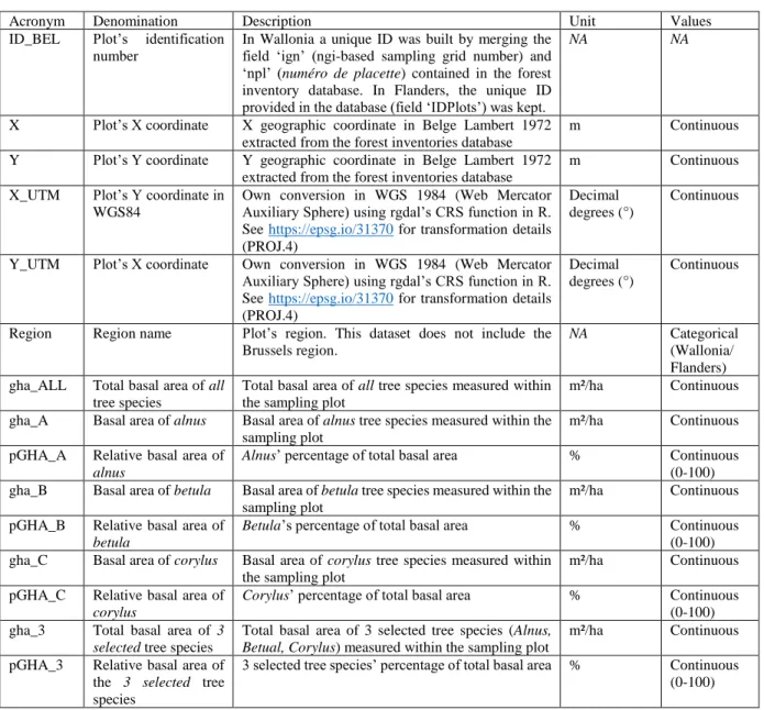
At the outset, we created a Belgian detaset where both Flemish and Walloon dataset were merged. A shapefile named ‘data_sp_BEL_pcGHA_FULL’ was built, which contains absolute and relative basal areas values (see table 7 below for variable details). The step-by-step computation method from R scripts can also be found in Appendix under the section named “ Belgian Forest Inventry (RespirIT_IF_BEL.R)”.

Table 8. Details on output variables

Acronym Denomination Description Unit Values ID_BEL Plot’s identification

number

In Wallonia a unique ID was built by merging the field ‘ign’ (ngi-based sampling grid number) and ‘npl’ (numéro de placette) contained in the forest inventory database. In Flanders, the unique ID provided in the database (field ‘IDPlots’) was kept.

NA NA

X Plot’s X coordinate X geographic coordinate in Belge Lambert 1972 extracted from the forest inventories database

m Continuous Y Plot’s Y coordinate Y geographic coordinate in Belge Lambert 1972

extracted from the forest inventories database

m Continuous X_UTM Plot’s Y coordinate in

WGS84

Own conversion in WGS 1984 (Web Mercator Auxiliary Sphere) using rgdal’s CRS function in R. See https://epsg.io/31370 for transformation details (PROJ.4)

Decimal degrees (°)

Continuous

Y_UTM Plot’s X coordinate Own conversion in WGS 1984 (Web Mercator Auxiliary Sphere) using rgdal’s CRS function in R. See https://epsg.io/31370 for transformation details (PROJ.4)

Decimal degrees (°)

Continuous

Region Region name Plot’s region. This dataset does not include the Brussels region.

NA Categorical (Wallonia/ Flanders) gha_ALL Total basal area of all

tree species

Total basal area of all tree species measured within the sampling plot

m²/ha Continuous gha_A Basal area of alnus Basal area of alnus tree species measured within the

sampling plot

m²/ha Continuous pGHA_A Relative basal area of

alnus

Alnus’ percentage of total basal area % Continuous (0-100) gha_B Basal area of betula Basal area of betula tree species measured within the

sampling plot

m²/ha Continuous pGHA_B Relative basal area of

betula

Betula’s percentage of total basal area % Continuous (0-100) gha_C Basal area of corylus Basal area of corylus tree species measured within

the sampling plot

m²/ha Continuous pGHA_C Relative basal area of

corylus

Corylus’ percentage of total basal area % Continuous (0-100) gha_3 Total basal area of 3

selected tree species

Total basal area of 3 selected tree species (Alnus,

Betual, Corylus) measured within the sampling plot

m²/ha Continuous pGHA_3 Relative basal area of

the 3 selected tree species

3 selected tree species’ percentage of total basal area % Continuous (0-100)

Nb: For basal area calculation details in Wallonia and Flanders see p.6 and p.10 respectively. For a discussion on data spatial coverage gaps in Flanders see p.11.

(18)

3.1.4. Results

3.1.4.1. Tree structure and tree mix

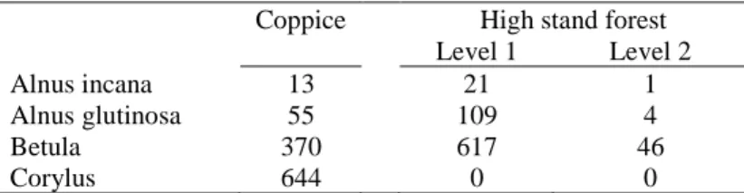
From the Walloon forest inventory dataset, details about the structure of trees can be provided. The table below shows that Alnus are mainly observed in the first level (highest level) of any stand structure (even-aged stand with one layer, even-aged stand with two layers or uneven-aged stand). Betula is also mainly observed in the first level (highest level) of any stand structure. Yet, an important number of trees are also observed under the form of coppice. Corylus on the opposite is only observed in stand structures with coppice (i.e. coppice stand, coppice with high stand or high stand with coppice).

Table 9. Number of observations based on the type of tree structure Coppice High stand forest

Level 1 Level 2

Alnus incana 13 21 1

Alnus glutinosa 55 109 4

Betula 370 617 46

Corylus 644 0 0

Tree species combine in various ways within each plot. Within the Walloon forest inventory dataset, we identified seven possibilities depending on how allergenic tree combine. In most cases (82%), plots contain one type of tree only. Almost one fifth (17%) of the plots contain a combination of two species. One percent only contains the three species studied.

Table 10. Combination of allergenic tree species in sampling plots

1 2 3 4 5 6 7 Alnus X X X X Betula X X X X Corylus X X X X TOTAL 83 682 433 44 28 169 14 % 82% 17% 1%

3.1.4.2. Presence-absence of allergenic trees

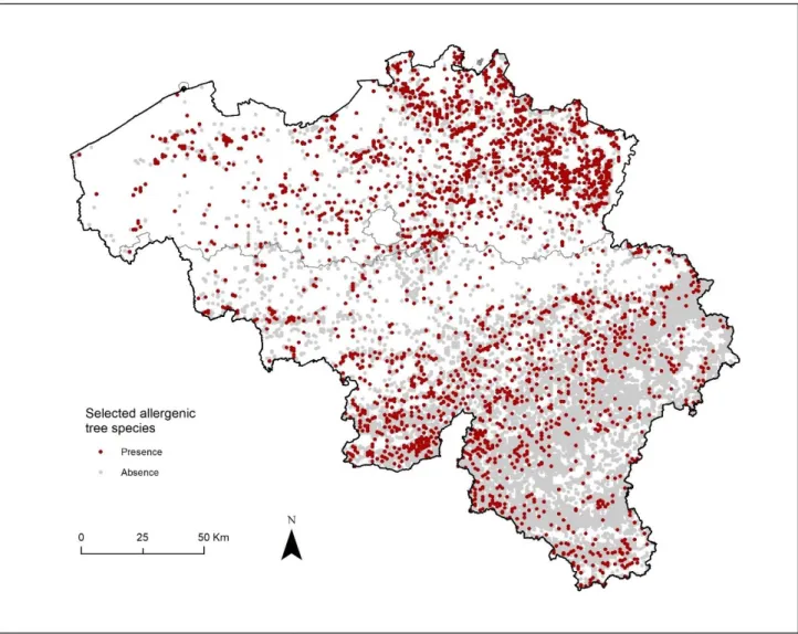
In Wallonia, most forest areas containing the three allergenic tree species studied (alnus, betula, corylus) are located in the southern part of the region. In particular, 90,9% of the sampling plots containing at least one allergenic tree species are located south of the “sillon Sambre et Meuse” (i.e. the former industrial axis running from the city of Mons to Liège through Charleroi and Namur). The highest densities of allergenic tree species can be observed on the northern border of the Ardenne

(19)

While the “plateau ardennais central” and the “plateau ardennais du nord-est” concentrate large forest areas, these areas are characterized by a low density of allergenic tree species. This may be related to the following factors: (i) soil types are not the best suited for the development of either Alnus, Betula or Corylus, and (ii) an important number of parcels only contain coniferous trees (e.g. “Haut plateau des Fagnes”, the German border area) where tree mix is less important. Meanwhile, areas containing the lowest density of allergenic trees in Wallonia are the “plateaux limoneux brabançons et hesbignons” were large parcels of agricultural land are dominant, leaving less space for forested areas.

Figure 4. Combined sampling plots from the Walloon and Flemish forest inventories with presence-absence of 3 selected allergenic trees (alnus, betula, corylus)

3.1.4.3. Relative share of allergenic trees

The relative share of allergenic trees was calculated as an important indicator for describing the importance and spatial distribution of allergenic trees throughout Belgium. This variable (named “pcgha”) represents the share of allergenic trees within the plot sampled calculated as percentage of the basal area. This percentage was first computed for each tree species individually. Then, all 3 values were summed up to provide an overall percentage.

(20)

As the violin plot below shows, alnus and betula present median values around 20% (red dots). The presence of corylus is even lower with median values lower than 5%. Histograms’ distributions (grey areas) show that a high proportion of plots contain very low shares of allergenic trees. When considering all tree species together, the average share rises to 15%. Such patterns suggest that allergenic trees species are most often combined with other (non-allergenic) trees species, which may offer a postitive effect by capturing the pollens emitted by the neighbour species.

Table 11 below summarises that allergenic trees are present within Belgian forest area in fairly low percentages with average basal areas ranging from 8,7% (Corylus) to 35,7% (Alnus). In total, 1.934 plots out of the 13.228 plots surveyed in the Flemish and the Walloon forest inventories contain at least one allergenic tree.

(21)

Table 11. Summary statistics

Sampling plots with/without allergenic trees

Average basal area (%)

Alnus Betula Corylus 3 selected

allergenic trees

Flanders 1.102 / 2.147 33,4 23,1 3,7 27,5

Wallonia 832 / 11.081 41,3 32,3 11,8 29,9

Total 1.934 / 13.228 35,7 27,0 8,7 28,5

3.1.5. Spatial distribution of alnus, betula and corylus

The following maps show the presence and absence of each tree species individually. A four-class categorisation using the quantile method was used to represent differences in the relative presence of the 3 selected allergnic trees. Note that a comparison of categories between species should be avoided as tresholds vary from one specie to another (see values’ distribution patterns within the violin plot above). Alnus is the less represented specie throughout the study area. Its spatial distribution presents a scattered pattern with no specific concentration at the regional level. No important densities are found in any of the sub-regions. Betula is more common throughout the country and presents higher densities. At the sub-regional level, it is well represented in the South of the “sillon Sambre et Meuse” and the northeast area of Flanders. The presence of Betula is often associated with major forested areas. The density of corylus is lower than Betula, but higher than Alnus. It is concentrated outside the major forested area. In Wallonia for instance, Betula is located outside the major productive forest areas from the “plateaux ardennais”.

(22)

Betula

Corylus

3.1.6. The spatial distribution of 3 selected allergenic tree species in Belgium

The following map pictures the spatial distribution of the percentage of all allergenic trees (variable “pcgha”). No clear pattern emerges as to describe where the highest and lowest percentages are located. The percentage of allergenic trees per plot is heterogeneous throughout the region. This suggests that the relative importance of allergenic trees relies more upon local factors such as soil types for instance.

(23)

(24)

3.2. Non-forest inventory data

Several options were explored for gathering data outside forested areas in this research.

• For the Brussels region, a well detailed vegetation inventory made by Bruxelles Evironnement – IBGE exist. A detailed inventory of presence-only tree species within the public domain is freely available upon request by the organisation but could not be processed in the framework of this project.

• Some project-specific initiatives also exist such as those undertaken during the RespiIT project. For instance, the KULeuven team undertook fieldwork using Durham samplers. Around each sampler, they searched for allergenic tree species in a 2 km radius (12,6km²). They surveyed 15 points during a search effort of 10 minutes with two people (= 0,33 person-hours). The total basal area and birch basal area were measured.

• The Flemish flora database provides a presence-only dataset available for Flanders at a 4km square resolution. The KUL team implemented a Specie Distribution Model (SMD) using Maxent with this data. The low resolution of this dataset did not allow for considering this source as a possible option for our mapping of allergenic tree species.

• Data recrods from Observations.be / Waarnemingen.be is a crowdousourcing platform where volunteers, researchers, and scientists share their plant and animal sightings.

The latter data source was considered as the best candidate for characterizing the presence-absence of allergenic tree species outside forested areas.

3.2.1. Observations.be / Waarnemingen.be

The non-profit organisation “Observation International” provides a website named Observation.org or with many regional aliases, including observations.be/.waarnemingen.be that can be accesed with client applications such as ObsMapp (Android), iObs (iOS) and WinObs (Windows). Builiding upon these platforms, volunteers, researchers and scientists can make field observations and report them at any time. The inclusion of such type of data into a global digital system creates a powerful tool for multiple applications, including conservation, research, policy, experience and education. The main objective of International Observation is “the optimum facilitation of observers in order to make their nature experience even more valuable”. Yet, records from such a type of initiatives are opportunistic, less structured and mostly incidental observations. They are often suspected to be information-poor

(25)

3.2.2. Number of records and frequency

As shown in table 12 and figure 5 below, an important diversity of tree specie records could be accessed freely for this research via the observations.org platform. A specific selection of the three targeted allergenic tree species for the 2008-2018 period could be imlplemented by selecting the most relevant species of Alnus, Betula, and Corylus.

Table 12. List of allergenic tree species

Species name (latin) Count

2 Alnus glutinosa 8.200

3 Alnus incana 1.014

1 Alnus cordata* 187

5 Alnus x pubescens (A. glutinosa x incana) 7 6 Alnus x spaethii (A. japonica x subcordata)* 4

4 Alnus spec. 235

8 Betula pendula 7.231

10 Betula pubescens 2.106

7 Betula papyrifera* 2

9 Betula pendula + Betula pubescens 481 12 Betula x aurata (B. pendula x pubescens) 7

11 Betula spec. 1.838 13 Corylus avellana 9.416 14 Corylus colurna* 31 15 Corylus maxima* 16 16 Corylus spec. 4 TOTAL 30.820

* Not considered for analysis

Figure 5. Frequency of opportunistic observations from the observations.org database for the 2008-2018 perdiod.

(26)

3.2.3. Spatial footprint

The spatial footprint of opportunistic observations covers the entire country (see Figure 6 below). The location of records extends way beyond forest areas. Many cities and densely populated areas contain an important number of observations from volunteers (see figure 7). Obsevations in city parks, suburban areas, and large infrastrcutures were also reported by participants. A small regional effect can be observed around the ‘Pays des collines’ – ‘Vlaamse Ardennen’ border, which may be explained by differences of behaviour between volunteers (differences of interest and/or levels of awareness about the obsevations.be initiative), but his effect disappears in the southern periphery of Brussels were observation are continuous from the center the periphery of the city. Higher point density areas also include recreational areas (e.g. forested areas around major cities, touristic valleys) and spaces located along transport infrastructures such as walkways and roads.

(27)

Figure 7. Detailed location of opportunistic observations from the observations.org database in the harbour of Antwerp (upper left), the city outskirst of Antwerp (upper right), the area of Namur city (lower left) and the coastal city of Niewport (lower right). Colours show the level of point occuracy (0-1000m).

(28)

3.2.4. Complementarity with forest inventories

Figure 8. Combined presence-only records from regional forest inventory dataset and obsevations.org database for the 3 selected allergenic tree speciess (alnus, betula, corylus)

(29)

4. Conclusions

Forest inventories provide a detailed account of tree species observed within forest areas. The plots sampled offer a high-resolution, up-to-date description of the selected allergenic tree species (Alnus, Betula, and Corylus) at the scale of a land parcel. This has great potential for ecological modelling because the share of tree species within a tree stand (in percent of the basal area or percent cover) is a key variable for measuring densities of allergenic trees and characteritze its relative abundance of within a forested land parcel. Our results showed that allergenic trees are present within forest areas in relatively low percentages: three-fourth of the sampling plots contain less than 45% of allergenic tree species. Most allergenic trees are observed in the north-eastern part of Flanders and the south of the “sillon Sambre and Meuse”. The country’s major productive forests do not concentrate the most important share of allergenic trees. The observation records from open citizen science initiatives such as the observations.org platform are opportunistic, less structured and mostly incidental observations. While they are often suspected to be information-poor compared to information-rich database from forest inventories, we showed here that they contain a greater number of records gathered at higher time frequency. The spatial footprint of allergenic tree records is much larger than forest inventories and covers many areas outside forested areas. This complementariy should be considered as an opportunity for building comprenhensive database of presence-absence database that can better serve the elaboration of Species Distribution Models (SDMs).

(30)

5. Cited references

AFDELING BOS & GROEN 2001. De bosinventarisatie van het Vlaamse Gewest. Resultaten van de eerste inventarisatie 1997-1999. Ministerie van de Vlaamse Gemeenschap.

ALDERWEIRELD, M., BURNAY, F., PITCHUGIN, M. & LECOMTE, H. Inventaire Forestier Wallon-Résultats 1994-2012. 2015. SPW.

ALLOUCHE, O., TSOAR, A. & KADMON, R. 2006. Assessing the accuracy of species distribution models: prevalence, kappa and the true skill statistic (TSS). Journal of applied ecology, 43, 1223-1232.

ELITH, J., GRAHAM, C. H., ANDERSON, R. P., DUDÍK, M., FERRIER, S., GUISAN, A., HIJMANS, R. J., HUETTMANN, F., LEATHWICK, J. R. & LEHMANN, A. 2006. Novel methods improve prediction of species’ distributions from occurrence data. Ecography, 29, 129-151.

ELITH, J. & LEATHWICK, J. R. 2009. Species distribution models: ecological explanation and prediction across space and time. Annual review of ecology, evolution, and systematics, 40, 677-697.

GUISAN, A., ZIMMERMANN, N. E., ELITH, J., GRAHAM, C. H., PHILLIPS, S. & PETERSON, A. T. 2007. WHAT MATTERS FOR PREDICTING THE OCCURRENCES OF TREES: TECHNIQUES, DATA, OR SPECIES'CHARACTERISTICS? Ecological monographs, 77, 615-630.

HEIKKINEN, R. K., MARMION, M. & LUOTO, M. 2012. Does the interpolation accuracy of species distribution models come at the expense of transferability? Ecography, 35, 276-288. HILL, L., HECTOR, A., HEMERY, G., SMART, S., TANADINI, M. & BROWN, N. 2017.

Abundance distributions for tree species in Great Britain: A two‐stage approach to modeling abundance using species distribution modeling and random forest. Ecology and Evolution, 7, 1043-1056.

HOPKINS, J. J. & KIRBY, K. J. 2007. Ecological change in British broadleaved woodland since 1947. Ibis, 149, 29-40.

MCINNES, R. N., HEMMING, D., BURGESS, P., LYNDSAY, D., OSBORNE, N. J., SKJØTH, C. A., THOMAS, S. & VARDOULAKIS, S. 2017. Mapping allergenic pollen vegetation in UK to study environmental exposure and human health. Science of the Total Environment, 599, 483-499.

PEARSON, R. G. & DAWSON, T. P. 2003. Predicting the impacts of climate change on the distribution of species: are bioclimate envelope models useful? Global ecology and biogeography, 12, 361-371.

PRENTICE, I. C., CRAMER, W., HARRISON, S. P., LEEMANS, R., MONSERUD, R. A. & SOLOMON, A. M. 1992. Special paper: a global biome model based on plant physiology and dominance, soil properties and climate. Journal of biogeography, 117-134.

R CORE TEAM 2015. R: A language and environment for statistical computing. R Foundation for Statistical Computing, Vienna, Austria. 2015.

RACKHAM, O. 2008. Ancient woodlands: modern threats. New Phytologist, 180, 571-586.

RONDEUX, J. & LECOMTE, H. 2010. Inventaire Permanent des Ressources Forestières de Wallonie-Guide méthodologique.

THUILLER, W. 2003. BIOMOD–optimizing predictions of species distributions and projecting potential future shifts under global change. Global change biology, 9, 1353-1362.

WOUTERS, J., QUATAERT, P., ONKELINX, T. & BAUWENS, D. 2008. Ontwerp en handleiding voor de tweede regionale bosinventarisatie van het Vlaamse Gewest. Report INBO.

(31)

1. Appendix: R scripts

1.1. Walloon Forest Inventory (RespirIT_IFW_5.R)

##################### SUMMARY ################################### # PACKAGES # OVERALL APPRAOCH # DATA IMPORT # DATA PROCESSING # PLOTTING # FINAL TABLE # MAPPING ##################### PACKAGES ###################################

library("rJava", lib.loc="~/R/win-library/3.3")

#library("xlsx", lib.loc="~/R/win-library/3.3") #! If activated > conflict with XLConnect

library("XLConnect", lib.loc="~/R/win-library/3.3")

library("reshape", lib.loc="~/R/win-library/3.3")

library("reshape2", lib.loc="~/R/win-library/3.3")

library("stringi", lib.loc="~/R/win-library/3.3")

library("stringr", lib.loc="~/R/win-library/3.3")

library("shapefiles", lib.loc="~/R/win-library/3.3")

library("plyr", lib.loc="~/R/win-library/3.3")

library("rgdal", lib.loc="~/R/win-library/3.3")

library("vioplot", lib.loc="~/R/win-library/3.3")

library("ggplot2", lib.loc="~/R/win-library/3.3")

#install.packages('ggplot2', repos='http://cran.rstudio.com', type='source')

library("shapefiles", lib.loc="~/R/win-library/3.3")

library("rgdal", lib.loc="~/R/win-library/3.3")

#.rs.restartR() ## FUNCTIONS ##

# Multiple plot function

multiplot <- function(..., plotlist=NULL, file, cols=1, layout=NULL) { library(grid)

# Make a list from the ... arguments and plotlist

plots <- c(list(...), plotlist)

numPlots = length(plots)

# If layout is NULL, then use 'cols' to determine layout

if (is.null(layout)) { # Make the panel

# ncol: Number of columns of plots

layout <- matrix(seq(1, cols * ceiling(numPlots/cols)), ncol = cols, nrow = ceiling(numPlots/cols)) } if (numPlots==1) { print(plots[[1]]) } else {

# Set up the page

grid.newpage()

pushViewport(viewport(layout = grid.layout(nrow(layout), ncol(layout))))

# Make each plot, in the correct location

for (i in 1:numPlots) {

# Get the i,j matrix positions of the regions that contain this subplot

matchidx <- as.data.frame(which(layout == i, arr.ind = TRUE))

print(plots[[i]], vp = viewport(layout.pos.row = matchidx$row, layout.pos.col = matchidx$col)) }

} }

##################### OVERALL APPROACH ############################ # Work on plots ("placettes" in french).

# Work on species ("essences" in french). # Variables creation (1 by 1)

# Operations (splitting, merging, aggregating, etc.) # Recompilation for export into shapefiles

# Data IMPORT (data_sp, data_pl) # DATA PROCESSING:

# Plots containing measured trees (A)

# Plots containing 1 non-measured tree or more (B) # (a) Approach per class

# (b) Approach by linear regression model # Merging both datasets (A & B)

# Plots containing only 1 tree (C1)

# Plots contraining more than one tree (C2) # C1_a) Plots with only one "Aulne" (or none) # C1_b) Plots with more than one "Aulne" # Re-building "data_spW__C2" (C2_a & C2_b)

# Aggregation over fut & tai for measured trees with more than 1 tree per plot (C2)

# Re-building "data_spW__C2" # Re-building "data_spW__C1" # Re-building "data_spW__C" # Caculating overall GHA values # a) Alnus, Betual, Corylus # b) All 3

# PLOTTING # MAPPING

(32)

##################### DATA IMPORT ###################################

setwd("C:/Users/dujardis/Documents UNamur/20160401 RespirIT")

# Sheet "Placettes"

# Describes the characteristics of each plot

# Tells us about where plots are located and what kind of general species are found (structure, peuplement).

temp<-loadWorkbook("C:/Users/dujardis/Documents UNamur/20160401

RespirIT/2_DATA/Inventaire forestier Wallon/20160902 IFW/Req_dujardin_010916_VF.xlsx")

data_plW<-readWorksheet(temp, sheet = "Placettes", startRow = 16)

# 1) ID_Pl

# Creation of a unique identifier for each plot

data_plW$ID_pl <- paste(data_plW[,"ign"],data_plW[,"npl"],sep="") data_plW$ID <- 1:nrow(data_plW) # Unique ID

#colnames(data_plW) #data <- c(ID_plW) #data <- data.frame(c(1:nrow(data_plW))) #colnames(data) <- c("ID_pl") data_plW$ID_X <- 0 data_plW$ID_Y <- 0 # 2) XY coordinates

# To identify the location of each plot,

# if there are GPS coordinates (x_gps/y_gps variable), then keep the GPS coordinates.

# If it is not available (NA), then use the "IGN grid coordinates" (x/y variable).

#ID_X

for(i in 1:nrow(data_plW)) {

if( !is.na(data_plW[i,"x_gps"])) {

data_plW[i,"ID_X"] <- data_plW[i,"x_gps"] }

else {data_plW[i,"ID_X"] <- data_plW[i,"x"] } } data_plW$ID_X # ID_Y #data$ID_Y <- 0 data_plW<- data_plW[, c( "ID",

"ID_pl", # Reorganizes "ID_pl" as first column

"ign", "npl", "cy", "tranche", "dg_datem", "ID_X", # move here

"ID_Y", # move here

"x", "y", "x_gps", "y_gps", "dg_prov", "province", "dg_rfor_2", "region", "dg_n2000", "stru_pl", "structure", "peup_pl", "peuplement", "NHAf", "GHAf", "VHAf", "NHAt", "GHAt", "VHAt", "LIS", "lisiere", "PHY_OBS1", "PHY_OBS2" )]

### Sheet "Essences" (tree species)

# Details de different types of tree species found wihtin each plot # Aulne = Alnus

# Bouleau = Betula # Noisetier = Corylus

temp<-loadWorkbook("C:/Users/dujardis/Documents UNamur/20160401

RespirIT/2_DATA/Inventaire forestier Wallon/20160902 IFW/Req_dujardin_010916_VF.xlsx")

data_spW <-readWorksheet(temp, sheet = "Essences",startRow = 9) data_spW$ID_pl <- paste(data_spW[,"ign"],data_spW[,"npl"],sep="")

(33)

## Reorganise

data_spW <- data_spW[, c( "ID",

"ID_pl", # move here

"ign", "npl", "cy", "source", "etg_f", "ess", "essence", "pcgha", "nha", "gha", "vha", "count" # "ess_mix", # "alnus_aggr" ) ] var_data_spW <- c( "ID",

"ID_pl", # move here

"ign", "npl", "cy", "source", "etg_f", "ess", "essence", "pcgha", "nha", "gha", "vha", "count" # "ess_mix", # "alnus_aggr" ) ######################### DATA PROCESSING ############################ ## Tree structure (Table)

temp_melt <- melt(data_spW, id = c("ID_pl", "ign", "npl", "cy", "source", "etg_f", "essence"))

table_spW_tree_str <- cast(temp_melt, essence ~ source + etg_f,

subset=variable=="count", sum)

table_spW_tree_str

<-table_spW_tree_str[,c("essence","tai_NA","fut_1","fut_2")] table_spW_tree_str

#Control check:

#temp <- data_spW[data_spW$essence== "Aulne blanc" & data_spW$source== "fut", ]

#temp <- data_spW[data_spW$essence== "Bouleau" & data_spW$source== "tai", ] ## Tree count

# How many different type of allergenic tree specie are recorded per plot? # > Count the number of duplicate "ID_pl" in "data_spW"

temp <- cast(temp_melt, ID_pl ~ variable, sum) # Aggregation per plot > Identification of duplicates

table(temp$count)

316+48+5 # Total number of plot with more than one type of allergenic tree

369/1453*100 # relative share (one fourth)

# Adding this variable the the dataset "data_spW"

data_spW$dupl <- 0

data_spW$dupl <- temp$count[match(data_spW$ID_pl, temp$ID_pl)]

# When only one tree type > no aggregation needed. Measures can be taken as it is

# When more than one > Need for aggregating measures depending on: # Alnus vs Betula vs Corylus

# tai vs fut 1 vs fut 2

## Assign a number from 1 to 11 identifying the pcgha class

# NB: This variable is not neccesary when using a "regression model approach" # See work on dataframe "data_spW" below

temp <- data_spW temp$pcgha_class <- 999

for(i in 1:nrow(temp)) {

if (temp[i,"pcgha"] > 0.99999) {

temp[i,"pcgha_class"] <- 11 # when pcgha = 1 (the specie is dominant)

}

else if (temp[i,"pcgha"] <= 0.99999999 & temp[i,"pcgha"] >= 0.90000000 ){ temp[i,"pcgha_class"] <- 10

}

(34)

}

else if (temp[i,"pcgha"] <= 0.99999999 & temp[i,"pcgha"] >= 0.00000001 ){ temp[i,"pcgha_class"] <- 1 } else { } } #table(temp$pcgha_class) data_spW <- temp

## Identifying whether plots contain measured trees or not # Loop over groups

temp <- data_spW

for(grp in unique(temp$ID_pl)) { # Group by 'ID_pl'

if(any(is.na(temp[temp$ID_pl == grp, 'gha']))) { # If a plot contains a 'gha' with no value (NA)

temp[temp$ID_pl == grp, 'measured'] <- 0 # Then assign 0

}

else {temp[temp$ID_pl == grp, 'measured'] <- 1 # Otherwise asign 1

} }

data_spW <- temp

## Plots containing measured trees (A)

data_spW__A <- data_spW[data_spW$measured==1,]

nrow(data_spW__A)

#any(is.na(data_spW__A$gha)) # Control to see if no NA values remains #table(is.na(data_spW__A$pcgha))

## Plots containing 1 non-measured tree or more (B)

data_spW__B <- data_spW[data_spW$measured==0,]

nrow(data_spW__B)

#count(is.na(data_spW__B$gha)) # 690/820 trees not measured

690/1879*100

## Processing plots containing 1 non-measured trees or more (B) # Idea of assigning an average 'gha' for non-measured trees

# Search for all measured trees within the dataset and determine was is the average 'gha' value

# !Make a difference between 'tai" and 'fut' 1 et 2

# !Make a difference between tree species (Alnus,Betula,Corylus)

temp <- data_spW[!is.na(data_spW$gha) & !is.na(data_spW$pcgha) ,] # Select observations were gha (& pcgha) is known

1189

temp$count <- 1

temp[,"essence"] <- gsub("Aulne glutineux", "Aulne", temp[,"essence"]) temp[,"essence"] <- gsub("Aulne blanc", "Aulne", temp[,"essence"])

temp_melt <- melt(temp, id = c("ID_pl", "ign", "npl", "cy", "source", "etg_f", "essence", "pcgha_class"))

#Tai #a. Count

temp_aggr <- cast(temp_melt, essence+pcgha_class ~ variable, sum, subset =

source=="tai")

count_alnus <- temp_aggr[temp_aggr$essence=="Aulne",9] # Count

count_alnus <- append(count_alnus, mean(count_alnus),5) # ! Alnus, cat. 6 = NA > Assign an average value

count_betula <- temp_aggr[temp_aggr$essence=="Bouleau",9] count_corylus <- temp_aggr[temp_aggr$essence=="Noisetier",9] means_count <- data.frame(count_alnus,count_betula, count_corylus)

#b. Mean

temp_aggr <- cast(temp_melt, essence+pcgha_class ~ variable, mean, subset =

source=="tai")

mean_alnus <- temp_aggr[temp_aggr$essence=="Aulne",7] # Mean gha

mean_alnus <- append(mean_alnus, mean(mean_alnus),5) # ! Alnus, cat. 6 = NA > Assign an average value value

mean_betula <- temp_aggr[temp_aggr$essence=="Bouleau",7] mean_corylus <- temp_aggr[temp_aggr$essence=="Noisetier",7] means_tai <- data.frame(mean_alnus,mean_betula, mean_corylus)

plot(means_tai$mean_alnus)

plot(means_tai$mean_betula)

plot(means_tai$mean_corylus)

# No obvious/strong linear correlation

# some means are based upon a single observation... # ! One pcgha category contains no observation (Alnus/6) #c. Min

#temp_aggr <- cast(temp_melt, essence+pcgha_class ~ variable, c(sum, mean, min, max), subset = source=="tai")

#Fut #a. Count

temp_aggr <- cast(temp_melt, essence+pcgha_class ~ variable, sum, subset =

source=="fut")

(35)

mean_alnus <- temp_aggr[temp_aggr$essence=="Aulne",7] # Mean gha

mean_betula <- temp_aggr[temp_aggr$essence=="Bouleau",7]

#temp_corylus <- temp_aggr[temp_aggr$essence=="Noisetier",7] # Not applicable (corylus does was not observed under the form of a tree stand)

means_fut <- data.frame(mean_alnus,mean_betula)

plot(means_fut$mean_alnus)

plot(means_fut$mean_betula)

#plot(means_mean$temp_corylus) #c. Min

#temp_aggr <- cast(temp_melt, essence+pcgha_class ~ variable, c(sum, mean, min, max), subset = source=="tai")

## Assigning 'means' to missing values

temp <- data_spW__B

table(temp$pcgha_class)

#Tai

j <- 1

while(j <= nrow(means_tai)){ for(i in 1:nrow(temp)) {

if (temp[i,"pcgha_class"] == rownames(means_tai[j,]) & is.na(temp[i,"gha"]) & temp[i,"source"]=="tai" & temp[i,"essence"]=="Aulne blanc"){

temp[i,"gha"] <- means_tai[j,"mean_alnus"] }

else if (temp[i,"pcgha_class"] == rownames(means_tai[j,]) & is.na(temp[i,"gha"]) & temp[i,"source"]=="tai" & temp[i,"essence"]=="Aulne glutineux"){

temp[i,"gha"] <- means_tai[j,"mean_alnus"] }

else if (temp[i,"pcgha_class"] == rownames(means_tai[j,]) &

is.na(temp[i,"gha"]) & temp[i,"source"]=="tai" & temp[i,"essence"]=="Bouleau"){

temp[i,"gha"] <- means_tai[j,"mean_betula"] }

else if (temp[i,"pcgha_class"] == rownames(means_tai[j,]) &

is.na(temp[i,"gha"]) & temp[i,"source"]=="tai" & temp[i,"essence"]=="Noisetier"){

temp[i,"gha"] <- means_tai[j,"mean_corylus"] } else { } } j <- j+1 } #Fut j <- 1

while(j <= nrow(means_fut)){ for(i in 1:nrow(temp)) {

if (temp[i,"pcgha_class"] == rownames(means_fut[j,]) & is.na(temp[i,"gha"]) & temp[i,"source"]=="fut" &

temp[i,"gha"] <- means_fut[j,"mean_alnus"] }

else if (temp[i,"pcgha_class"] == rownames(means_fut[j,]) & is.na(temp[i,"gha"]) & temp[i,"source"]=="fut" & temp[i,"essence"]=="Aulne glutineux"){

temp[i,"gha"] <- means_fut[j,"mean_alnus"] }

else if (temp[i,"pcgha_class"] == rownames(means_fut[j,]) &

is.na(temp[i,"gha"]) & temp[i,"source"]=="fut" & temp[i,"essence"]=="Bouleau" ){

temp[i,"gha"] <- means_fut[j,"mean_betula"] } else { } } j <- j+1 } data_spW__B <- temp

# (b) Approach by linear regression model

# Idea of establishing a statistical relationship between pcgha and gha values based on measured obervations

# Building a linear regression model per structure (tai/fut) and species (Alnus, Betula, Corylus) allows predicting gha for non measured observations

# !Need to distinguish observations with pcgha = 1 (the specie is dominant) and where pcgha < 1

# b1 (pcgha < 1): Predicted value provided by the linear regression model # b2 (pcgha < 1): Average value

temp <- data_spW[!is.na(data_spW$gha) & !is.na(data_spW$pcgha) ,] # Select observations were gha (& pcgha) is known

temp[,"essence"] <- gsub("Aulne glutineux", "Aulne", temp[,"essence"]) # All types of alnus are considered the same

temp[,"essence"] <- gsub("Aulne blanc", "Aulne", temp[,"essence"]) # All types of alnus are considered the same

temp <- temp[temp$pcgha_class!=11,] # selecting where pcgha < 1 #temp2 <- temp[temp$pcgha_class==1,] # selecting where pcgha = 1 #Tai

tai_alnus <- temp[temp$source=="tai"& temp$essence=="Aulne", ] pcgha <- tai_alnus$pcgha

gha <- tai_alnus$gha

plot(pcgha, gha, main="Scatterplot", xlab="pcgha ", ylab="gha ", pch=19)

cor(gha,pcgha)

#cov(gha,pcgha)

model_tai_alnus <- lm(gha~0+pcgha) # Regression through the origin (i.e. intercept=0)

model_tai_alnus

summary(model_tai_alnus) # R² = 0,632

abline(model_tai_alnus)

Research note on mapping allergenic tree species distributions in Belgium

RESEARCH OUTPUTS / RÉSULTATS DE RECHERCHE

Author(s) - Auteur(s) :

Publication date - Date de publication :

Permanent link - Permalien :

Rights / License - Licence de droit d’auteur :

Institutional Repository - Research Portal

Dépôt Institutionnel - Portail de la Recherche

researchportal.unamur.be

BRAIN-be

BR/154/A1/RespirIT

Research note on mapping allergenic tree species

in Belgium

14/04/2017

Updated on 26/02/2021

Dr. Sébastien Dujardin

Pr. Catherine Linard

Pr. Nicolas Dendoncker

Table of contents

1. Introduction

2. Dataset inventory

3. Allergenic tree species distributions

4. Conclusions

5. Cited references

1. Appendix: R scripts