W boson measurement in the muonic decay channel at forward rapidity with ALICE

HAL Id: tel-01639163

https://tel.archives-ouvertes.fr/tel-01639163

Submitted on 20 Nov 2017

HAL is a multi-disciplinary open access

archive for the deposit and dissemination of sci-entific research documents, whether they are pub-lished or not. The documents may come from teaching and research institutions in France or

L’archive ouverte pluridisciplinaire HAL, est destinée au dépôt et à la diffusion de documents scientifiques de niveau recherche, publiés ou non, émanant des établissements d’enseignement et de recherche français ou étrangers, des laboratoires

forward rapidity with ALICE

Jianhui Zhu

To cite this version:

Jianhui Zhu. W boson measurement in the muonic decay channel at forward rapidity with ALICE. Nu-clear Theory [nucl-th]. Ecole nationale supérieure Mines-Télécom Atlantique, 2017. English. �NNT : 2017IMTA0014�. �tel-01639163�

Mémoire présenté en vue de l’obtention du

grade de Docteur de IMT ATLANTIQUE sous le sceau de l’Université Bretagne Loire École doctorale : 3MPL

Discipline : Constituants élémentaires et physique théorique Spécialité : Physique des Ions Lourds

Unité de recherche : Subatech, Nantes, France Soutenue le 01 avril 2017

Thèse N° : 2017IMTA0014

Mesure de la production du boson W dans le

canal muonique à rapidité à l’avant avec ALICE

W boson measurement in the muonic decay

channel at forward rapidity with ALICE

JURY

Rapporteurs : Nicole BASTID, Professeur, LPC, Université Clermont Auvergne, France

Yugang MA, Professeur, Shanghai Institute of Applied Physics, CAS, Chine

Examinateurs : Zhongbao YIN, Professeur, Central China Normal University, Chine

Xiaoming ZHANG, Chargé de Recherche, Central China Normal University, Chine

Co-encadrant : Daicui ZHOU, Professeur, Central China Normal University, Chine

Directeur de Thèse : Ginés MARTINEZ-GARCIA, Directeur de Recherche CNRS, Subatech, Ecole des Mines-Telecom, France

rapidité à l’avant avec ALICE

Ré mé

Selon le modèle standard, la matière est constituée de particules fondamentales : les quarks, les leptons et les bosons médiateurs d’interaction. Les quarks sont les particules soumises à l’interaction forte, qui est véhiculée par les gluons, et peuvent avoir six saveurs différentes. Les leptons et les

quarks sont soumis à l’interaction électrofaible, véhiculée par les bosons W±_{, Z}0_{et les photons.}

Le modèle standard explique de nombreux résultats et prédit l’existence d’une particule, le bo-son de Higgs, qui est responsable de la masse des autres particules. Dans le modèle standard, l’interaction forte entre les quarks et les gluons (partons) est décrite par la théorie de la Chro-moDynamique Quantique (QCD). La constante de couplage de l’interaction forte change avec l’énergie/distance entre particules. Elle est notamment grande à petites impulsions/grandes dis-tances et petite à grandes impulsions/petites disdis-tances. Par conséquent, les partons sont confinés dans les hadrons (confinement), mais ils se comportent comme des particules quasi-libres à petites distances et hautes énergies d’interaction (liberté asymptotique). Les calculs de QCD sur réseau

(lattice-QCD) prédisent que, dans des conditions extrêmes de densité d’énergie (& β GeV/fm3₎

et/ou densité numérique des baryons (& β fm−3_{), les partons ne sont plus confinés à l’intérieur}

des hadrons (déconfinement), et un nouvel état de la matière est formé, constitué par quarks et gluons : le Plasma de Quarks et de Gluons (QGP). Ce nouvel état de la matière était le plus abondant lors de premières microsecondes après le Big Bang et pourrait exister aujourd’hui au cœur des étoiles à neutrons où la densité du nombre baryonique est très élevée. L’étude du QGP donne donc des informations importantes sur l’interaction forte, les propriétés de la matière à très haute température et l’évolution de l’univers lors de ses premiers instants.

Les conditions pour la formation du QGP peuvent être reproduites en laboratoire à travers la collision d’ions lourds ultra-relativistes. Deux faisceaux d’ions lourds, accélérés à une vitesse très proche de la vitesse de la lumière, s’entrechoquent créant dans la zone de la collision des densités d’énergie extrêmement élevées qui peuvent mener à la formation du QGP. Le QGP créé va subir d’une violente expansion relativiste dans le vide qui entoure la zone de la collision. Lors de cette

expansion, la densité d’énergie du milieu diminue et en quelques dizaines de fm/

clemilieusecon-fine en produisant une matière hadronique (gaz de hadrons). Bien qu’il soit impossible d’observer les QGP directement, certaines observables bien précises ont la particularité d’être très sensibles

la production de photons et de dileptons. En revanche la production de boson électrofaibles ne devrait pas être affectée par la présence du QGP et représente une référence unique qui n’a jamais été mesurée dans les collisions entre ions lourds avant la construction du grand collisionneur de hadrons au CERN.

En général, le taux de production de particules ou leurs distributions cinématiques peuvent être modifiés par la présence du QGP par rapport aux observations faites dans les collisions proton. Toutefois, certaines modifications par rapport à la production en collisions proton-proton ne sont pas dues à la présence d’un milieu deconfiné, mais à des effets liés à l’utilisation des ions lourds, telle que la modification de la fonction de distribution partonique (PDF) dans les noyaux (comme le shadowing, la saturation de gluons, etc).

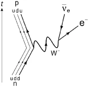
À cause de sa grande masse, le boson W est produit lors des collisions partoniques dures dans la phase initiale de la collision des noyaux, avant la formation du QGP. Ses produits de désin-tégration leptoniques ne sont pas affectés par la présence du milieu deconfiné, car ils ne sont pas sensibles à l’interaction forte. Il s’agit donc d’un canal idéal pour la compréhension des ef-fets nucléaires non liées au QGP. En particulier, la mesure des bosons vecteurs dans un large intervalle en rapidité permet d’étudier les PDF nucléaires (nPDF) dans une région de haute

vir-tualitéQ2

∼ (β00 GeV)2et de fraction d’impulsion du parton dans le nucléon (x-Bjorken) qui est

actuellement peu contrainte par les données. En outre, l’étude de l’asymétrie de charge des bosons

W±_{, qui sont produits principalement lors des processus}u¯d → W+_etd¯u → W−_{à hautes}

éner-gies, permet de tester la dépendance des modification des PDFs par rapport à la saveur des quarks. En collision proton-proton, le taux de production du boson W est bien connu, et sa mesure peut être donc utilisée comme chandelle standard pour l’estimation de la luminosité. Comme pour les collisions Pb–Pb, la fonction de distribution partonique en collisions proton-plomb est affectée par les effets nucléaires tels que le shadowing et la saturation de gluons. Par conséquent, l’étude de boson W est très importante pour comprendre la distribution partonique dans le noyau.

Le Grand Collisionneur de Hadrons (LHC) de l’Organisation Européenne pour la Recherche Nucléaire (CERN) qui se trouve à Genève en Suisse fonctionne depuis γ009 et il a produit des

collisions en proton-proton à des énergies du centre de masse de√s = 7, 8 et βδ TeV, des

colli-sions proton-plomb à des énergies par nucléon de √sNN= 5.0γ et 8.β6 TeV ainsi que des collisions

plomb-plomb à γ.76 et 5.0γ TeV. Le LHC a marqué un nouveau chapitre dans le domaine de la physique des hautes énergies. L’énergie du centre de masse atteinte au LHC est jusqu’à γ5 fois plus grande que celle atteinte par le Relativistic Heavy Ion Collider (RHIC) au Laboratoire

Na-d’énergie.

ALICE (A Large Ion Collider Experiment) est la seule parmi les 4 expériences installées au LHC à être spécifiquement conçue pour la physique des ions lourds. Elle est constituée d’un ton-neau central complété par un spectromètre à muon vers l’avant ainsi que des détecteurs pour les mesures à grandes rapidités. Le spectromètre à muon couvre la région de pseudo-rapidité −4.0 <

η < −γ.5. Encollisionproton-proton,

leréférentielducentredemassecoïncideavecceluidulab-oratoire et on mesure donc des muons avec une rapidité entre −4.0 < ycms < −γ.5. En collision

proton-plomb, par contre, la différence d’impulsion entre le proton et l’ion mène à une dévia-tion de la rapidité du système de centre de masse. En renversent la direcdévia-tion de circuladévia-tion des

deux faisceaux, il est donc possible de mesurer des muons avec γ.0δ < ycms <δ.5δ (protons

voy-ageant vers le spectromètre) et −4.46 < ycms < −γ.96 (protons s’éloignant du spectromètre).

On note aussi que la région de rapidité couverte par le spectromètre à muon d’ALICE est com-plémentaire de celle des expériences ATLAS et CMS. Le spectromètre à muons se compose d’un aimant dipolaire avec un champ magnétique intégré de δ T.m de cinq stations de trajectographie composées de chambres proportionnelles multifils à lecture bi-cathodique et de deux stations de déclenchement composées de chambres à plaques résistives et de plusieurs éléments d’absorption. Les stations de trajectographie sont placées en aval d’un absorbeur frontal conique en carbone, béton et acier, d’une longueur épaisseur de 4.β m (correspondant à β0 longueurs d’interaction nu-cléaire) qui filtre les hadrons, électrons et photons produits au point d’interaction. Les stations de déclenchement sont placées après une paroi de fer d’une épaisseur de β.γ m (7.γ longueurs d’interaction) qui absorbe les hadrons secondaires s’échappant de l’absorbeur et des muons de faible impulsion, provenant principalement de la désintégration des hadrons légers. Enfin, un blindage de faisceau conique recouvrant le tube faisceau protège le spectromètre des particules produites lors de l’interaction des particules de grande rapidité avec le tube lui-même.

La centralité de la collision est mesurée à partir de l’énergie déposée dans calorimètre à zéro dégrée pour neutrons (ZN) en direction de l’ion de plomb qui se fragmente. Le nombre moyen

de collisions nucléon-nucléon binaires < Ncoll >est obtenu à partir de la “méthode hybride”,

qui se repose sur l’hypothèse que la multiplicité mesurée des particules chargées à mi-rapidité

est proportionnelle au nombre moyen de nucléons qui participent à la collision < Npart >. Les

valeurs de < Npart >pour une classe de centralité ZN donnée sont calculées en mettant à l’échelle

le nombre moyen de participants dans des collisions MB < NMB

part >, estimé avec un Glauber

mi-Npart >pour indiquer l’hypothèse utilisée pour la mise à l’échelle. Le nombre correspondant

de collisions binaires est alors obtenu comme: < Nmult

coll >=< Nmultpart > −β. Les incertitudes

systématiques sont estimées en utilisant différentes hypothèses.

Cette thèse a pour objectif, la mesure de la production du boson W vers l’avant dans le canal muonique en collisions proton-plomb à 5.0γ TeV et proton-proton à 8 TeV avec l’expérience ALICE au LHC. Pour les collisions proton-plomb, la production de bosons W a été également étudiée en fonction de la centralité de la collision. Il s’agit de la première mesure du boson W à grandes rapidités en collisions proton-plomb. Dans ce travail, nous avons tout d’abord étudié les caractéristiques cinématiques des muons issus de la désintégration du boson W par des

simula-tions, afin d’en extraire sa contribution à la distribution d’impulsion transverse (pT). On observe

que la contribution est maximale pourpT ∼ 40 GeV/c. A plus basse impulsion transverse la

source principale de muons est la désintégration des hadrons contenant un quark charmé ou beau. A haute impulsion transverse la contribution principale du bruit de fond est constituée

par des muons issus de la désintégration de Z0_/ ∗_{. La distribution cinématique des différentes}

contributions est décrite par des “templates” obtenues avec des simulations MC qui utilisent des calculs de QCD comme générateur. La contribution du signal est obtenue en ajustant les don-nées avec ces templates. Le nombre de muons ainsi estimé est corrigé par l’acceptance et l’efficacité du détecteur et normalisé pour obtenir la section efficace. L’asymétrie de charge, définie comme le rapport entre la différence de production des muons positifs et négatifs sur la production to-tale, est mesurée également. Les mesures sont comparées avec des calculs de QCD perturbative au Next-to-Leading Order (NLO) et Next-to-Next-to-Leading Order (NNLO). Les résultats en collisions proton-proton sont en bon accord avec la théorie (Figure β). Dans le cas des collisions

cms µ y 5 − −4 −3 −2 −1 0 1 2 3 4 5 (pb) σ 300 400 500 600 700 800 900 1000 = 8 TeV s ALICE, pp @ c > 10 GeV/ T µ p , Data + W ← + µ , Data W ← -µ , POWHEG, CT10 + W ← + µ , POWHEG, CT10 W ← -µ This thesis

Figure 1:Section efficace de muon avec unpμ_T > β0GeV/cprovenants de la décroissance du bosonsW±dans les

colli-sions pp à 8 TeV. La mesure a été comparée à la prédiction obtenue avec le logiciel POWHEG en utilisant les fonction de distribution de partons CT10.

nucléaires des PDFs. Les mesures expérimentales sont compatibles avec les deux cas dans les in-certitudes actuelles (Figure γ). En collision proton-plomb, on mesure aussi la section efficace de la production de muons issus de la désintégration des bosons W divisée par le nombre moyen de collision nucléon-nucléon, en fonction de la centralité de l’événement, déterminée avec différents estimateurs. Comme la production du boson W est proportionnelle aux collisions nucléon-nucléon, son taux de production par collision nucléon-nucléon devrait être constant en fonction de la centralité si les estimateurs ne sont pas biaisés. La mesure montre que la dépendance est plate pour tous les estimateurs dans les incertitudes expérimentales qui sont entre 8 et β6% (Figure δ).

ALI-PUB-118937

Figure 2:Section efficace différentielle en rapidité des muon positifs depμ_T >β0GeV/cprovenant de la décroissance du

bosonW+_{. Les mesures sont comparées aux modèles théoriques incluant ou pas les effets de shadowing des fonctions des}

distribution des partons selon la paramétrisation EPS09.

Centrality class 0-100% 2-20% 20-40% 40-60% 60-100% (nb)〉 coll mult N〈 / W ← µ σ 20 22 24 26 28 30 32 34 36 = 5.02 TeV NN s ALICE, p-Pb > 10 GeV/c µ T p < 3.53 cms y 2.03 < Global uncertainty: 4.3% ALI-PUB-118953

Figure 3:Section efficaces des muons depμ_T > β0GeV/cprovenant de la décroissance du boson W normalisé par les

nombre de collisions binaires, en fonction de la centralité de la collision proton-plomb. La centralité a été estimée par un les calorimètre à zéro degrés ZN.

de physique des hautes énergies, le chapitreβintroduit principalement le modèle standard et le

diagramme de phase de la matière nucléaire et le chapitreγse focalise sur la théorie électrofaible,

la motivation de physique de la présente thèse. Le chapitreδprésente les principes de

concep-tion des détecteurs d’ALICE et l’utilisaconcep-tion des différents sous-détecteurs et le chapitre4montre

l’acquisition et le traitement des données. Le chapitre5décrit la méthode d’extraction des signaux

du boson W dans les données en collisions proton-plomb et dans le chapitre6la même méthode

est utilisée pour l’analyse en collisions proton-proton. Le chapitre7est un résumé des résultat

obtenus et les perspectives de ces études.

En conclusion, cette thèse présente la première mesure des bosons W avec le détecteur ALICE. Dans les collisions proton-proton, les calculs théoriques reproduisent correctement les mesures qui ont des incertitudes entre 8 et β6%. Dans les collisions proton-plomb, les calculs théoriques des collisions nucléon-nucléon renormalisés par le nombre de collisions binaires reproduisent également les données. Toutefois, les calculs tenant compte du shadowing des gluons dans le noyau de plomb semblent être un meilleur accord avec les mesures, notamment à rapidité positive où les effets du shadowing devraient être plus importants. L’étude de la production de boson W en fonction de la centralité de la collision p–Pb a permis de vérifier la loi d’échelle avec le nombre de collisions nucléon-nucléon avec une précision de β5%. Certains résultats de ce travail de thèse ont été publiés dans la revue Journal of High Energy Physics, volume β70γ, page 77 par la collaboration ALICE avec le titre “W and Z boson production in p–Pb collisions at 5.0γ TeV”. Mots-clés : Collisions d’ions lourds; Collisions d’hadrons; Plasma de Quarks et de Gluons (QGP); Grand Collisionneur de Hadron (LHC); A Large Ion Collider Experiment (ALICE); Or-ganisation Européenne pour la Recherche Nucléaire (CERN); Boson électrofaible; Muon; Fonc-tion de distribuFonc-tion des partons; Collisions proton - plomb; Collisions proton - proton

rapidity with ALICE

A

With the beginning of the Large Hadron Collider (LHC) at CERN in γ009, a new era in Quark-Gluon Plasma (QGP) physics has started by studying heavy-ion collisions at high ener-gies in the centre of mass frame (γ5 times larger than those in the RHIC collider at BNL). The LHC represents today an ideal tool to study the properties of QGP in the laboratory. ALICE (A Large Ion Collider Experiment) is the only experiment of LHC specifically designed to measure those properties. A wide variety of observables can be studied by means of the β8 sub-detectors of the ALICE apparatus, which are grouped in two main elements: the central barrel and the muon spectrometer. With the muon spectrometer, we can detect high transverse momentum muons and dimuons in order to measure open heavy flavours, quarkonia and electroweak bosons pro-duction.

The high collision energies available at the LHC allow for an abundant production of hard

probes, such as quarkonia, high-pT jets and vector bosons (W, Z), which are produced in

ini-tial hard parton scattering processes. The latter decay before the formation of the QGP, which is a deconfined phase of Quantum ChromoDynamics (QCD) matter produced in high-energy heavy-ion collisions. Furthermore, their leptonic decay products do not interact strongly with the QGP. The electroweak bosons provide a way for benchmarking in-medium modifications to coloured probes. In Pb–Pb and p–Pb collisions, precise measurements of W-boson produc-tion can constrain the nuclear Parton Distribuproduc-tion Funcproduc-tions (nPDFs), which could be modified with respect to the nucleon due to shadowing or gluon saturation. In addition, they can be used to test the scaling of hard particle production with the number of binary nucleon–nucleon col-lisions. Especially in p–Pb collisions, the measurement of W yields at forward and backward

rapidity allows us to probe the modification of nPDFs at small and large Bjorken-x, respectively.

Such measurements can be benchmarked in pp collisions, where W-boson production is theoret-ically known with good precision. Also, the charge asymmetry of leptons from W-boson decays is a sensitive probe of up and down quark densities in a nucleon inside a nucleus.

ALICE has already completed data taking of large data samples of pp collisions at√s = 7, 8

and βδ TeV, p–Pb collisions at √sNN= 5.0γ TeV and Pb–Pb collisions at √sNN= γ.76 and 5.0γ TeV.

production of W-boson in pp collisions at 8 TeV and p–Pb collisions at 5.0γ TeV are measured

with the ALICE muon spectrometer via the inclusivepT-differential muon yield. In pp collisions

the rapidity covered by muon spectrometer is −4 < yμ

cms < −γ.5 and in p–Pb collisions it

separates into forward rapidity (p-going direction, γ.0δ < yμ

cms < δ.5δ) and backward rapidity

(Pb-going direction, −4.46 < yμ

cms < −γ.96) via changing beam direction. These rapidity

regions are complementary to the one of ATLAS (A Toroidal LHC ApparatuS, |ηlab| < γ.5) and

CMS (Compact Muon Solenoid, |ηlab| < γ.4) experiments.

This thesis consists of four parts. PartIis the introduction of high-energy physics and

con-tains two chapters. Chapterβis a general knowledge of QCD and QGP, and Chapterγ

concen-trates on the electroweak theory and the motivation of investigating of W-boson in heavy-ion

collisions. PartIIpresents the ALICE experiment, which involves hardware, software, the online

data taking and the offline data selection. Chapterδshows the design of the structure including

central barrel and forward muon spectrometer and Chapter4gives an account of data. PartIII

is the core content, which reveals the detail of W-boson measurement in p–Pb (Chapter5) and

pp (Chapter6) collisions. Finally, the conclusions are drawn in partIV(Chapter7).

Keywords: Heavy ion collisions; HIC; Hadronic collisions; Quark Gluon Plasma; QGP; LHC; ALICE; CERN; Electroweak boson; Muon; Parton distribution functions; PDF; Nuclear parton distribution functions; nPDF; p–Pb collisions; pp collisions; 5 TeV; 8 TeV

Acknowledgments

I would like to express my gratitude to all those who helped me during the writing of this thesis. My deepest gratitude goes first and foremost to all my supervisors, Daicui Zhou at CCNU in Wuhan (China), Gines Martinez and Diego Stocco at SUBATECH in Nantes (France), for their constant encouragement and guidance during my PhD career. Especially thank Diego for his experience, useful discussions and excellent ability in data analysis.

I am indebted to Philippe Pillot for discussions on the resolution of muon tracks, which is the challenge of this thesis. Also thank Francesco Bossu and Kgotlaesele Johnson Senosi for their collaboration and cross-check step by step in the analysis. I’m also grateful to Zaida Conesa Del Valle and Francesco Prino for their suggestions and comments during the research. I appreciate Yugang Ma and Nicole Bastid for carefully reading this manuscript and providing useful com-ments and suggestions.

High tribute shall be paid to Nicole Bastid and Philippe Crochet for their discussions in muon analysis and help in life when i was in Clermont-Ferrand from August to December, γ0ββ. My cordial and sincere thanks go to the whole member of ALICE group at Nantes, Laurent Aphecetche, Guillaume Batigne, Marie Germain, Alexandre Shabetai, Astrid Morreale, Javier Martin, Lucile Ronflette, Benjamin Audurier and etc for their warm help during my stay in Nantes.

I am also very grateful to all member of ALICE group at Wuhan, Zhongbao Yin, Xiaoming Zhang, Yaxian Mao, Hua Pei, Dong Wang, Fan Zhang, Xiangrong Zhu, Mengliang Wang, Ru-ina Dang, Shuang Li, Jiebin Luo, Liang Zheng, Hui Li, Wenzhao Luo, Xinye Peng, Xiaowen Ren, Yonghong Zhang, Zuman Zhang, Haitao Zhang, Hongsheng Zhu and etc for discussions in analysis and help in my daily life.

Special thanks should go to China Scholarship Council (CSC) and France China Particle Physics Laboratory (FCPPL) to provide me the funding support for stay in Nantes.

Last but not the least, big thanks go to my family who has shared with me my worries, frus-trations, and hopefully my ultimate happiness in eventually finishing this thesis.

Contents

I Introduction

β

β Particle physics in heavy-ion collisions γ

β.β Standard model . . . γ

β.β.β Quantum ChromoDynamics . . . 5

β.β.γ Lagrangian of QCD . . . 6

β.β.δ QCD phase diagram . . . 9

β.γ Heavy-ion collisions . . . ββ

β.γ.β The Big Bang . . . βγ

β.γ.γ Evolution of heavy-ion collisions . . . βδ

β.γ.δ Heavy-ion facilities . . . β4

β.γ.4 Characteristic of collisions and experimental observables . . . β6

γ Weak bosons in heavy-ion collisions δ0

γ.β Discovery of weak bosons . . . δ0

γ.γ Formation and decay . . . δγ

γ.γ.β Generation of weak boson . . . δ4

γ.γ.γ Parton distribution functions . . . 4β

γ.γ.δ W muonic decay channel . . . 46

II ALICE Experiment

49

δ The ALICE experiment 50

δ.β The Large Hadron Collider . . . 50

δ.γ ALICE setup . . . 5γ

δ.δ Global detectors . . . 57

δ.5 Forward muon spectrometer . . . 6γ

δ.5.β The absorbers . . . 65

δ.5.γ The dipole magnet . . . 67

δ.5.δ The tracking chambers . . . 69

δ.5.4 The trigger chambers . . . 7δ 4 Data taking in ALICE 78 4.β ALICE online control system . . . 78

4.β.β Trigger (TRG) system . . . 79

4.β.γ Data AcQuisition (DAQ) system . . . 8β 4.β.δ High-Level Trigger (HLT) . . . 8γ 4.β.4 Detector and experiment control system . . . 8δ 4.γ ALICE offline framework . . . 85

4.γ.β Simulation . . . 88

4.γ.γ Reconstruction . . . 90

4.γ.δ Offline conditions database framework . . . 90

4.γ.4 ALICE computing grid . . . 9β

4.δ MUON quality assurance . . . 9γ

III W-boson Measurement

98

5 W-boson measurement in p–Pb collisions 99

5.β Data samples and standard cuts . . . β00

5.γ Analysis strategy . . . β0δ

5.δ Monte Carlo simulations . . . β0δ

5.4 Signal extraction . . . β05

5.4.β Heavy-flavour decay background description . . . β05

5.4.γ Fitting procedure . . . β07

5.4.δ Optimization of fitpTrange . . . β07

5.5 Acceptance × efficiency correction . . . ββ5

5.6 Normalisation to the number of minimum bias events . . . ββ6 5.7 Systematic uncertainties . . . ββ7

5.7.γ The component of Z0_/ ∗

→ . . . βγ0

5.7.δ Alignment effect . . . βγ0

5.7.4 Tracking/trigger efficiency . . . βδδ

5.7.5 Pile-up effect . . . βδ5

5.7.6 Combination of fit results . . . βδ8

5.7.7 Summary of systematic uncertainties . . . β4β

5.8 Results . . . β4γ

5.8.β Production cross section . . . β4γ

5.8.γ Charge asymmetry . . . β44

5.8.δ Cross section vs. centrality . . . β47

6 W-boson measurement in pp collisions β49

6.β Data sample . . . β49 6.γ Monte Carlo simulations . . . β5β 6.δ Signal extraction . . . β5δ 6.4 Acceptance × efficiency correction and normalization . . . β55 6.5 Results . . . β55

6.5.β Production cross section . . . β55

6.5.γ Charge asymmetry . . . β57

IV Discussions and Conclusions

β59

7 Conclusion β60

Appendix A Appendix β6γ

A.β Data samples in p–Pb collisions . . . β6γ A.γ Data sample in pp collisions . . . β6δ A.δ POWHEG . . . β64

Appendix B Publication List β69

Appendix C Presentation List β70

Part I

wμνcμ one s sure one s cεpεble. Only wμen we do not μεve to be εccountεble to εnyone cεn we find joy νn scνentνfic endeεvor.

Albert Einstein

1

Particle physics in heavy-ion collisions

During my doctoral career, the top three questions I have been asked are: what is a “particle”? why do you study it? how to use it in our daily life? I was perturbed each time when I chatted with my friends on my major. It is difficult to use simple words to explain what we researched to them since they do not have background in this field. Particles can not be seen with our own eyes and belong to the microscopic world, which means a special way is needed to investigate their physical properties. Many scientists began to think about how to describe particles via physical formula and how to design experimental devices to measure them. Thus, a lot of physical models were proposed in theory and some huge machines were built in experiment. So far, the most successful and a well-tested theory in particle physics is the Standard Model (SM). Let us start by describing what is the SM.

β.β Standard model

All matter is made of elementary particles which arise in two basic types called quarks and leptons, shown in the left panel of Figure β.β. Each of them consists of six particles, which are organized in “generations”. The lightest and most stable particles build up the first generation (quarks: up and down, leptons: electron and electron neutrino), while the heavier and less stable particles belong to the second generation (quarks: charm and strange, leptons: muon and muon

neutrino) and third generation (quarks: top and bottom, leptons: tau and tau neutrino). All stable matter in the universe is made of particles that belong to the first generation; any heavier particles quickly decay to the most stable level. Quarks and leptons have their antiparticles with the same mass and opposite charge named anti-quarks and anti-leptons, respectively.

Figure 1.1:The SM of elementary particles (left) and summary of interactions between particles described by the SM

(right).

In the broadest sense, a particle is a quantity of matter. In physics, a particle is a small object to which can be ascribed several physical properties such as charge or mass. We have already learned in the earlier schools that matter is made of atoms and atoms are made of smaller constituents: protons, neutrons and electrons. Protons and neutrons are made of quarks, while electrons are not. As far as we know, quarks and electrons are fundamental particles, not made of anything smaller. You can not have half an electron or one-third of a quark. And all particles of a given type are precisely identical to each other: they have little license plates that distinguish them. Any two electrons with the same energy will produce the same result in a detector, and that’s what makes them fundamental: they do not come in a variety pack.

The SM of particle physics (formulated in the β970s) describes the world in terms of particles (fermions, with fractional spin) and forces (which are mediated by bosons, with integer spin). Fermions obey a statistical rule described by Enrico Fermi (β90β–β954) from Italy, Paul Dirac (β90γ–β984) from England, and Wolfgang Pauli (β900–β958) from Austria called the exclusion principle. Simply stated, fermions can not occupy the same quantum state at the same time (two fermions can not be described by the same quantum numbers). All quarks and leptons, as well as any composite particle made of an odd number of these, are fermions. Bosons, in contrast, have no problem occupying the same quantum state at the same time (more formally, two or more

bosons may be described by the same quantum numbers). The statistical rules that bosons obey were first described by Satyendra Bose (β894–β974) from India and Albert Einstein (β879–β955) from Germany. As the particles that make up light and other forms of electromagnetic radia-tion, photons are the bosons we have the most direct experience with. All of these are described by Quantum Field Theory.

There are four fundamental forces in the nature: the strong force, the weak force, the elec-tromagnetic force and the gravitational force. They work at different ranges and have different strengths. Gravity is the weakest force and has an infinite range (as well as the electromagnetic force). It is accurately described by the general theory of relativity proposed by Albert Einstein

in β9β5 [β]. Gravity is not included in the SM, which is actually a fundamental problem that has

to be solved. However for the practical purposes of particle interactions, the effect of gravity is so weak to be negligible. The other three fundamental forces described by exchange of force-carrier particles, which belong to the family of bosons, are shown in the right panel of Figure β.β. The strong force is carried by the gluon, the weak force is carried by the W and Z bosons and the electromagnetic force is carried by the photon. These force-carrier particles are called “gauge bosons”. The electromagnetic interaction and the weak interaction in SM are described as two different aspects of a single electroweak interaction. This theory was developed around β968 by Sheldon Glashow, Abdus Salam and Steven Weinberg, and they were awarded the β979 Nobel prize in physics for their contributions to the theory of the unified weak and electromagnetic in-teraction between elementary particles, including, inter alia, the prediction of the weak neutral current.

The Higgs boson was the last missing piece of the SM puzzle. It is a different kind of force carrier from the other elementary forces, and it gives mass to quarks as well as the W and Z bosons. Whether it also gives mass to neutrinos remains to be clarified. Its existence has been confirmed by two experiments (ATLAS and CMS) on the Large Hadron Collider at CERN (European

Or-ganization for Nuclear Research*_{) on 4 July γ0βγ. This experimental discovery of Higgs boson}

[γ,δ] led that the Nobel prize in physics was awarded jointly to Professors Francois Englert and

Peter Higgs for the prediction of this fundamental particle on 8 October γ0βδ .

*_{The abbreviation ”CERN” is denominated according to its old name in French, Conseil Europeen pour la}

β.β.β Quantum ChromoDynamics

Quantum ChromoDynamics (QCD) is a type of quantum field theory [4] called a

non-abelian gauge theory with symmetry group SU(δ) that describes the strong interactions between quarks and gluons. In QCD, the analogous of the electric charge is a property called ”color”. There are three kinds of color charges, which are called red, green and blue, using the same ter-minology for colors perceived by humans. They are just quantum parameters and completely unrelated to familiar phenomenon of color in daily life. The quarks carry only one color, while the gluons are a combination of color and anti-color. The fact that the gluon carries a color charge is a fundamental difference compared to photons, since it allows for self-interaction. There are

eight different gluon types which form a SU(δ) octet [5] :

R¯G, R¯B, G¯R, G¯B, B¯R, B¯G,_√γ(Rβ _{R − G¯G),}¯ _√β

6(R¯R + G¯G − γB¯B)

The combination of color and anti-color for gluons and how a gluon changes the color of

quarks are shown in Figure β.γ. The symmetric singlet state _√δ(Rβ _{R + G¯G + B¯B) does not exist}¯

because it can not mediate color. All observed particles do not carry a net color charge and they are white or colorless.

Figure 1.2:The combination of color and anti-color for gluons (a), and how a gluon changes the color of quarks (b).

The peculiarities of QCD are:

• coupling constant larger than unity • confinement phenomena

• gluons carry colour and the asymptotic freedom

• spontaneous breaking to the chiral symmetry in the limit of zero-mass quark

β.β.γ Lagrangian of QCD

The QCD Lagrangian is given by [6]

L =∑

q

¯

ψ_q,a(ν μ∂μ ab− λs μtCabACμ − mq ab)ψ_q,b −_4Fβ AμνFAμν (β.β)

The μ_{are the Dirac -matrices; theψ}

q,aare quark-field spinors for a quark of flavor q and

massmq, with a color-indexε that runs from ε = β to Nc = δ, i.e. quarks have three “colors”;

ACare gluon fields with C running from β toN2c − β = 8, i.e. there are eight kinds of gluons

and they transform under the adjoint representation of the SU(δ) color group; thetC

abare eight

δ × δ matrices and are the generators of the SU(δ) group; the quantity λs(orαs = λ

2

s

4π) is the

QCD coupling constant. The couplingλs(orαs) and the quark massesmqare the fundamental

parameters of QCD. Finally, the field tensorFA

μνis given by

FA

μν = ∂μAAν − ∂νAAμ − λsfABCABμACν (β.γ)

where the structure constants of the SU(δ) groupfABCare

[tA,tB] =νf_ABCtC (β.δ)

Three useful color-algebra relations include:

tA abtAbc=CF ac (CF ≡ (N2c − β)/(γNc) =4/δ) fACDfBCD =CA AB (CA ≡ Nc =δ) tA abtBab =TR AB (TR=β/γ) (β.4)

CFandCAare the color-factors (“Casimir”) associated with gluon emission from a quark and

a gluon respectively.TRis the color-factor for a gluon to split to aq¯q pair.

The last term in Eq. β.γ makes a fundamental dynamical difference between QCD and Quan-tum EletroDynamics (QED), which leads to self-interactions between the gluons and asymptotic

freedom.

β.β.γ.β Confinement and asymptotic freedom

In physics, a coupling constant or gauge coupling parameter is a number that determines the strength of the force in an interaction. In QCD, the strong interaction is governed by a strong

coupling constantαsdefined as:

αs(Q2) = 4π (ββ − γ δnf)ln( Q 2 Λ2 QCD) (β.5)

whereQ2_{is the momentum transferred in the interaction,n}

fis the number of light flavors

withmq ≪ Q and ΛQCDis the non-perturbative QCD scale. The intensity of the strong

interac-tion decreases at short distances and increases when quarks move apart as observed in Figure β.δ.

Figure 1.3:Summary of measurements ofα_sas a function of the energy scale Q. The respective degree of QCD perturbative

theory used in the extraction ofα_sis indicated in brackets (NLO: next-to-leading order; NNLO: next-to-next-to leading

order; res. NNLO: NNLO matched with resummed next-to-leading logs; N3LO: next-to-NNLO) [6].

Therefore, the behavior of this running coupling constant provides two peculiarities of QCD.

For small values ofQ2_{, i.e. at large distances or small energies,α}

sbecomes large. On the contrary,

at small distance or large transferred momentum,αsbecomes weak, quarks and gluons behave as

free particles, which is known as asymptotic freedom [7,8]. This was first proposed by David

J. Gross, Frank Wilczek and H. David Politzer in β97δ who shared the Nobel Prize in physics in γ004.

In the region where the transferred momentum is large (the distance of interaction is small), physical observations can be calculated by truncated series like leading order (LO), next-to-leading order (NLO) and so on. The perturbative QCD (pQCD) was proven to describe the high

en-ergy interaction with high accuracy. On the other hand, at small transverse momentapT(large

distances) the strong coupling has large values and quarks are confined in neutral color states, the mesons and the baryons. This is well described by Lattice QCD calculations, which uses a non-perturbative approach in solving the QCD equation in a lattice of space and time.

β.β.γ.γ Chiral symmetry breaking and restoration

A chiral phenomenon is one that is not identical to its mirror image. In particle physics, the spin is used to define a handedness. The helicity of a particle is right-handed if the direction of its spin is the same as the direction of its motion. While it is left-handed if the directions of spin and motion are opposite (Figure β.4). Mathematically, the helicity of left-handed is negative, for right-handed it is positive. A symmetry transformation between the left-right-handed and right-right-handed is called parity. Invariance under parity by a Dirac fermion is called chiral symmetry.

Figure 1.4: Illustration of the helicity of a spin 1/2 particle as being left or right-handed.

Considering QCD with two massless quarksu and d, Eq. β.β can be written:

L = ∑

q=u,d

¯

ψ_q,a(ν μ∂μ ab− λs μtCabACμ)ψ_q,b− _4Fβ AμνFAμν (β.6)

It is invariant under the chiral transformation:

ψ → eiθγ5

ψ (β.7)

where θ is the generator of SU(γ) group. Note that gluon fields are not affected by chiral trans-formations, so gluon degrees of freedom can be neglected for the present discussion. In terms of

left-handed and right-handed spinors, the chiral transformation becomesSU(γ)L × SU(γ)R. If

additional quark flavors are taken into account, the dimensionality of the chiral group increases,

i.e., when three quarksu, d and s are considered the chiral group is SU(δ)L× SU(δ)R. This

sym-metry of the Lagrangian is called flavor chiral symsym-metry.

As a matter of fact, it turns out that when we consider the non-zero values of the quark

massesmu ≃ γ.δ MeV and md ≃ 4.8 MeV, chiral symmetry is explicitly broken. The origin of

the symmetry breaking may be described as an analog to magnetization, the fermion condensate (vacuum condensate of bilinear expressions involving the quarks in the QCD vacuum). The chiral condensation is defined as:

< ¯ψψ >=< ¯ψ_Lψ_R+ ¯ψ_Rψ_L > (β.8)

whereψ_L/Rare spinors of left- and right-handed particles. In the vacuum, < ¯ψψ ≯= 0,

the quark mass is non-zero and the chiral symmetry is spontaneously broken. But at high energy

one expects a restoration of the chiral symmetry, which is predicted for light quarks (u, d and s)

not for heavier quarks (c, b and t), < ¯ψψ >= 0. In this case the quarks recover their

almost-null mass of the QCD Lagrangian instead of their constituent mass, of the order of ∼ δ00 MeV

[9]. According to the chiral symmetry breaking the QCD explains the existence of the eight

Goldstone bosons (π0_,π+_,π−_,K0_,K+_,K−_{, ¯K}0_,η

8) with small mass values.

The principal and obvious consequence of this symmetry breaking is the generation of 99% of the mass of nucleons, and hence the bulk of all visible matter, out of very light quarks. For

example, for the proton, of massmp =9δ8 MeV, the valence quarks, withmu≃ γ.δ MeV, md ≃

4.8 MeV, only contribute by about 9 MeV to its mass, the bulk of it arising out of QCD chiral symmetry breaking, instead. Yoichiro Nambu was awarded the γ008 Nobel prize in physics for his understanding of this phenomenon.

Due to the restoration of the chiral symmetry, a phase transition of hadronic matter would be expected.

β.β.δ QCD phase diagram

As discussed above, quarks and gluons can not be observed directly at low energy, as they are confined inside colorless bound states (hadrons). However, QCD indicates that at high energy and/or baryonic density the strongly interacting matter undergoes a phase transition to a state where quarks and gluons are not confined into hadrons: the quark-gluon plasma (QGP). In the

phase diagram of QCD, the transition between the hadronic and QGP phases is not well known either theoretically or experimentally. A commonly conjectured form of the phase diagram in

terms of the temperature T as a function of the baryonic-chemical potential _B is depicted in

Figure β.5.

Figure 1.5: Schematic phase diagram of QCD matter in the plane of temperatureTand baryonic-chemical potential _B

[10].

To perform calculations in the regime of high temperature and large coupling strength and to research a phase transition from normal hadronic matter to deconfined QCD matter, the lattice

QCD theory was created. It has been performed for two-flavor (u, d) and three-flavor (u, d, s)

quarks to establish the equation of state of nuclear matter. Figure β.6 shows the energy density

scaled by the temperature to the fourth power /T4_{as a function of temperature divided by the}

critical temperatureT/Tc. It indicates a phase transition from hadronic matter to the QGP at

a critical temperature ofTc ≈ β70 MeV ≈ β012 K at _B = 0 and at an energy density c ≈

β GeV/fm3_{. Such temperatures were present in the early phase of the evolution of the universe,}

at about β s after the Big Bang. On the other hand, density exceeding the above critical value is

also conjectured to be present in the interior of compact, dense stellar objects, such as the neutron

Figure 1.6: The evolution of the scaled energy density as a function ofT/T_cfrom Lattice QCD calculation [11].

β.γ Heavy-ion collisions

The QGP can be produced in laboratory through ultra-relativistic heavy-ion collisions. The Relativistic Heavy Ion Collider (RHIC) and the Large Hadron Collider (LHC) operate at high energies, where the initial excess of quarks over antiquarks is negligible compared to the total number of created particles and the crossing time for heavy-ion collisions is much smaller than the formation time for the plasma, resulting in a low net baryon density. On the other hand, various experiments at lower energies aim to study the system at large net densities, for example RHIC II or the future Facility for Antiproton and Ion Research (FAIR) in Darmstadt (Ger-many). One of the most important objectives in the latter experiments is to identify a possible critical endpoint on the phase diagram, beyond which the transition becomes of first order. De-veloping our theoretical understanding of the QCD phase diagram can prove highly beneficial for designing these next generation experiments.

According to the “Big Bang” theoretical model, in few microseconds after the big bang, the universe was filled with a hot, dense soup made of all kinds of particles moving at near light speed. This mixture was dominated by quarks and gluons. In those first moments of extreme temperature, however, quarks and gluons were bound only weakly, free to move on their own in QGP. Historically, T. D. Lee in collaboration with G. C. Wick first speculated about an abnor-mal nuclear state, where nucleon mass is zero or near zero in an extended volume and non-zero

is through high-energy heavy-ion collisions. To recreate conditions similar to those of the very early universe, powerful accelerators make head-on collisions between massive ions, such as gold or lead nuclei. In these heavy-ion collisions the hundreds of protons and neutrons inside such

nuclei smash into one another at energies of a few β012_{electron volts each. The QGP is formed}

in these collisions.

β.γ.β The Big Bang

The Big Bang theory is the prevailing cosmological model for the universe from the earliest

known periods through its subsequent large-scale evolution [βδ,β4]. According to the prospect

of hot Big Bang Model [β5], the universe expanded from a very high density and high temperature

state that occurred about βδ.7 billion years ago, which happened att ∼ β0−11_{s after the big bang,}

and then the temperature went down during the expansion. After one Planck time of expansion, a phase transition caused a cosmic inflation, during which the Universe grew exponentially. As the inflationary period ends, the Universe consists of a QGP, which is the main focus of the

heavy-ion physics. When the expansheavy-ion continued until the temperature dropped to β012 _{K, quarks}

began to combine into protons, neutrons and other baryons. As time progressed, some of the protons and neutrons formed deuterium, helium, and lithium nuclei. Later, electrons combined with protons and these low-mass nuclei to form neutral atoms. Due to gravity, clouds of atoms contracted into stars, where hydrogen and helium fused into more massive chemical elements. Exploding stars (supernovae) form the most massive elements and disperse them into space. Our earth was formed from supernova debris. Figure β.7 shows the time evolution of the universe from the big bang to the present time.

Figure 1.7:The evolution of the universe.

The purpose of the research on the high-energy physics is not only to understand the proper-ties of particles and the interaction between them but also to investigate how the universe began and expanded. How can we recreate the conditions that were present at the early universe?

For-tunately, physicists have found the answer by designing and building powerful accelerators to perform ultra-relativistic heavy-ion collisions.

β.γ.γ Evolution of heavy-ion collisions

As presented in Figure β.8, the evolution of an ultra-relativistic heavy-ion collision can be summarized as follows:

Figure 1.8: Top four figures: schematic view of the various stages of a heavy-ion collision. The thermometers indicate when

thermal equilibrium might be attained. (a) the two nuclei before the collision, (b) the formation of a QGP if a high enough

energy density is achieved, (c) the later hadronization, (d) free-streaming of the hadrons towards the detectors. [9] Bottom

figure: sketch of the evolution of heavy-ion collisions in space and time. [16].

in the direction of the incoming heavy-ion beams due to Lorentz contraction and are as-sumed as pancake in the laboratory frame.

• Pre-equilibrium: a lot of inelastic nucleon-nucleon collisions occur in the overlap region of the colliding nuclei and a large amount of energy is deposited near the collision point. Hard processes happen first and shortly after that soft processes take place. Partons are

produced within this high-energy density environment via hard processes (τ ∼ 0). The

pre-equilibrium state lasts for a typical time scaleτ ∼ β fm/c. By partons interaction, both

high and lowpTobjects are created during this process. The multiple scattering among

constituent quarks and gluons and between particles created during the collisions lead to a rapid increase in the entropy in the system which could eventually lead to equilibrium.

These initial processes among partons can be divided into two parts [β7]: hard processes

which have large momentum transferQ (Q ≫ ΛQCD), short timescale and a production

cross section that is proportional to the number of binary collisions (σhard ∝ Ncoll); soft

processes which have smallQ, long timescale and a production cross section proportional

to the number of participants (σsoft ∝ Npart). The majority of particles comes from soft

processes.

• QGP formation and thermalization: a rapid increase in the entropy could lead to thermal-ization and the temperature rises rapidly. If the attained energy density exceeds a critical energy density, the QGP might be formed.

• Hadronization and Freeze-out: after QGP formation, the system tends to expand and cools down towards a hadronic phase. During this procedure, a “mixed phase” is expected to exist between the QGP phase and hadronic phase. When the energy density is too low to allow inelastic collisions to create particles, the chemical freeze-out is attained. The sys-tem continues to increase its extent and gets colder; at some point the elastic collisions are no longer possible and the system reaches the kinetic freeze-out. At this moment the fireball disintegrates and hadrons escape.

β.γ.δ Heavy-ion facilities

Experimental attempts to create the QGP in the laboratory and measure its properties have been carried out for more than 40 years, by studying collisions of heavy nuclei and analyzing the

fragments and produced particles emerging from such collisions. During that period, center of

mass energy per pair of colliding nucleons (√sNN) have risen steadily as follows:

• β975-β985: √sNN ∼ γ GeV at the Bevalac at Lawrence Berkeley National Laboratory (LBNL)

[β8,β9,γ0,γβ]

• β987-β995: √sNN ∼ 5 GeV at the Alternating Gradient Synchrotron (AGS) at Brookhaven

National Laboratory (BNL) [γβ]

• γ000-now: √sNN ≤ γ00 GeV at the Relativistic Heavy Ion Collider (RHIC) at BNL. Four

experiments, PHENIX, STAR, BRAHMS and PHOBOS, are operated at this facility. [γβ]

• β987-now: √sNN ≤ 450 GeV at the Super Proton Synchrotron (SPS) accelerator at CERN

[γβ]

• γ009-now: √sNN ≤ 5.0γ TeV at the Large Hadron Collider (LHC) at CERN

One of the earliest experiments of heavy-ion collisions dates back to Bevalac at LBNL. The heavy-ion collisions with higher energies were carried out in the AGS at BNL for Au nuclei at

√sNN = 5 GeV and the SPS at CERN for Pb nuclei at √sNN = β7 GeV. Those accelerators

were fixed-target experiments and the energies were not sufficient to fully produce the QGP. The construction of the RHIC collider at BNL allowed to significantly increase the collision

energy, delivering pp, d-Au, Cu-Cu, Cu-Au and Au-Au collisions up to √sNN =γ00 GeV. The

results of the experiments at RHIC show that a hot and dense matter is created, thus providing a strong indication of the creation of the first human-made QGP. With the beginning of the heavy-ion program at the LHC at CERN, heavy-ion physics has entered a new energy regime.

LHC has delivered Pb-Pb collisions at √sNN = γ.76 TeV (in γ0ββ) and √sNN = 5.0γ TeV (in

γ0β6). It is believed that the properties of the hot medium does not fundamentally change from

RHIC to LHC [γγ,γδ], though several intriguing anomalies are reported in particle production

[γ4, γ5]. The analyses of azimuthal anisotropy show that the medium still behaves as a fluid

with small viscosity, which is important information since it has been naively expected that the QGP becomes slightly more weakly-coupled with increasing energy due to the QCD asymptotic freedom.

Some of the mentioned heavy-ion facilities together with the typical parameters related to particle production in nucleus-nucleus collisions and global features of the produced systems are summarized in Table β.β.

Parameters SPS RHIC LHC

Beam type Pb-Pb Au-Au Pb-Pb

√sNN(GeV) β7 γ00 γ760 dNch/dy|y=0 500 850 β600 τ0 QGP(fm/c) ∼ β ∼ 0.γ ∼ 0.β TQGP/Tc β.β β.9 δ-4.γ ε(at β fm/c) (GeV/fm3) _{∼ δ ∼ 5} β5 τQGP(fm/c) ≤ γ γ-4 ≥ β0 τf(fm/c) ∼ 4 ∼ 7 ∼ β0 Vf(fm3) ∼ β03 γ − δ × β03 ∼ 5 × β03 B(MeV) γ50 γ0 ∼ 0

Process soft → semi-hard → hard

Table 1.1:Global features of the medium created at SPS, RHIC and LHC energies [26,27]. From top to bottom, the

follow-ing quantities are presented: center of mass energy per nucleon pair (√s_NN), the charged-particle density at mid-rapidity

(dN_ch/dy|y=0), the equilibration time of the QGP (τ0QGP), the ratio of the QGP temperature to the critical temperature

(T_QGP/Tc), the energy density (ε), the lifetime of the QGP (τQGP), the lifetime of the system at freeze-out (τf), the volume

of the system at freeze-out (V_f), the baryonic chemical potential ( _B).

β.γ.4 Characteristic of collisions and experimental observables

As discussed in Section β.γ.γ, the two nuclei collide nearly at the speed of light and are squeezed

in the direction of beam axis in the laboratory frame. At RHIC energy, √sNN = γ00 GeV,

Lorentz dilation factor is ∼ β00 for a projectile nuclei, which means the nucleus of diameter

∼ β4 fm is reduced to ∼ 0.β fm. At the LHC energy√sNN =5.0γ TeV, ∼ γ500 and the nucleus

is squeezed to ∼ 0.005 fm. The hot medium would be produced in the overlapping area between the two passing nuclei. The collision axis is conventionally chosen as z-axis, and often referred to as the longitudinal direction as opposed to the transverse plane, which is perpendicular to the collision axis. In non-central collisions, the resulting geometry of a hot medium is elliptic in the transverse direction. The schematic pictures of the collision geometry of symmetric nuclei are shown in Figure β.9.

β.γ.4.β Coordinate system

It is more convenient to introduce the relativisticτ − η_scoordinate system to describe the

Figure 1.9: Schematic pictures of the geometry of non-central heavy-ion collisions with the longitudinal relativistic expan-sion (left) and the transverse expanexpan-sion (right).

τ =√t2_{− z}2

ηs= _γβlnt_{t − z}+z

(β.9) are the proper time and the space-time rapidity. The space-time rapidity is a dimensionless

variable that can be interpreted as a hyperbolic angle. They satisfy the relationst = τcoshηsand

z = τsinhηs. ηs = 0 corresponds to thet axis and η = ±∞ corresponds to the light cone.

Similarly, one defines the transverse massmTand the rapidityy in momentum space as

mT=√E2− p2z

y = _γβlnE+pz

E − pz

(β.β0)

In heavy-ion collisions, the transverse momentumpT =√m2T− m2and the pseudo-rapidity

η = _γβln(|p|+pz

|p| − pz)are useful variables because they are independent of mass. At relativistic

energies, they are quite close to the transverse mass and the rapidity, respectively, and become identical in the relativistic massless limit.

The polar coordinate system is often employed in analyses of the transverse dynamics. The

angle in the configuration space is denoted asφ and in the momentum space as φ_p. They are

re-lated to the variables in Cartesian coordinates as (x, y) = (rcosφ, rsinφ)and(px,py) = (pTcosφ_p,pTsinφ_p).

β.γ.4.γ Centrality

A collision can be very different if the heavy ions collide head on or just graze each other. In particular, the multiplicity of the produced particles increases from peripheral to central

colli-sions. In order to describe the dynamics of the nucleus-nucleus collision process, the collisions are classified into different centrality classes, which are related with the impact parameter. The

geometrical overlap region is parameterized by the impact parameter “b”, defined as the distance

between the central points of the colliding nuclei. The degree of centrality “C” of a given subset

of collisions can be indicated as a function of the corresponding cut-off of the impact parameter

“bc”:

C =

∫ bc

0 γπbdb

σinel (β.ββ)

whereσinelis the total inelastic cross section of a nucleus-nucleus collision. It represents the

probability that a collision occurs atb < bc. The centrality percentile can be quantified by the

pure geometry of the impact parameter via optical Glauber model [γ8]. Figure β.β0 presents the

schematic view of a collision with the optical Glauber model.

Figure 1.10: Schematic representation of the Optical Glauber Model geometry, with transverse (a) and longitudinal (b)

views. [28].

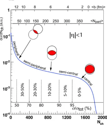
Since the impact parameter is not directly measurable, experimentally one usually uses ob-servables like the number of produced charged particles as shown in Figure β.ββ or the number

of participants † _{to classify centralities. Usually the central collisions refer to collisions with}

0 < C < 0.β and the peripheral collisions correspond to collisions with 0.9 < C < β. The

nuclei involved in the primary collisions are called “participants” and their total number

indi-cated asNpart, and others are called “spectators”. The total number of binary nucleon-nucleon

†_{The number of spectators (N}

collisions is indicated asNcoll.

Figure 1.11: A cartoon example of the correlation of the final-state observableN_chwith Glauber calculated quantities (b,

Npart). The plotted distribution and various values are illustrative and not actual measurements. [28].

The spectators will go through the collision region keeping their initial velocity as shown in

Bjorken’s model [γ9] of Figure β.βγ.

The average number of nucleon-nucleon collisions < Ncoll >at an impact parameterb is

given by < Ncoll(b) >=< TAA > (b)σNN, whereσNNis the total proton-proton inelastic cross

section andTAAis the nuclear thickness function, defined as:

TAB(b) = ∫ TA(s)TB(s − b)d2s (β.βγ) where TA(s) = ∫ ρA(s, z)dz (β.βδ)

The nucleon distribution inside the nucleus is assumed to follow a Woods-Saxon density profile:

ρA(s) = ρ0

β + exp(s − s0

ε )

Figure 1.12: The rapidity distribution of particles in heavy-ion collisions. Top: before collisions. Middle: after collisions with Landau’s full stopping model. Bottom: after collisions with Bjorken’s model.

wheres is the distance from a given point of the nucleus to the center of the nucleus. The

parametersε and s0are obtained empirically from electron scattering experiments. The Glauber

model [γ8] provides a quantitative description of the geometrical configuration of the nuclei

when they collide and basically describe the nucleus-nucleus interaction in terms of the elemen-tary nucleon-nucleon cross sections. For each centrality, the geometric parameters of

nucleus-nucleus collisions (Npart,Ncoll,TAA(b), b) are estimated with this model.

β.γ.4.δ Experimental observables

Theoretically the rough process of the evolution has been assumed and a series of mod-els, functions and formula have been created to calculate and explain physical phenomenons in heavy-ion collisions. While experimentally the only things we can see are digital signals of detector response caused by various types of particles like protons, neutrons, pions, kaons, elec-trons, muons, photons. Through technical analysis these different particles can be identified. Deservedly they become the probes that let us to infer the properties and phases of the matter

formed in the collisions and can be classified as global, initial and final state observables [δ0].

colli-sions such as the centrality, the reaction plane, the volume, the expansion velocity and the initial energy density. These quantities can be inferred from the measurement of the charged particle multiplicity, the transverse energy and the hadrons kinematics (among others). The collision centrality can be obtained from measurements of particle multi-plicity and of the energy carried by spectator nucleons. Moreover, studies of the transverse energy as a function of centrality carry information about the energy density, duration and opacity of the fireball.

• Initial-state observables: the probes which are not affected by the QGP formation are considered as initial-state observables. This means that they have the same behavior in the presence of cold nuclear matter (p-A collisions) and the QGP (A-B collisions).

Elec-troweak bosons include high-pT , W±and Z0are considered as initial-state probes as they

do not interact strongly. The particularities and interest of weak bosons will be further dis-cussed in Chapter γ. For what concerns photon production, different processes must be distinguished. On one hand, there are direct photons, which can be separated as prompt photons coming from the initial hard collisions and thermal photons emitted in the sec-ondary collisions either in the QGP phase or the hadronic phase. On the other hand, there

are decay photons, mainly fromπ and η decays, more than direct photons quantitatively.

• Final-state observables: The final-state observables provide information about the QGP and hadronic phase, which are obtained from the hadron yields and kinematic properties. There are many probes related to this kind of observables like the transverse momentum

distribution and the relative yield of the hadron species, the high-pTparticle correlations,

the flow and so on.

It is worth mentioning that hard probes are defined as high-energy probes produced in the

hard partonic scattering in the initial stage of the collision [δβ]. The production of hard probes

involves a large transfer of energy-momentum at a scaleQ ≫ ΛQCD. Such hard probes include

the production of Drell-Yan dileptons, massive gauge bosons, heavy quarks, prompt photons,

high-pTpartons observed as jets and high-pThadrons.

β.γ.4.δ.β Charged-particle spectra

The hadron yield is an indispensable observable to study heavy-ion collisions since hadrons constitute the bulk of the produced medium. Due to the strong interaction in the medium, the

pTspectra of charged particles as shown in the top panel of Figure β.βδ is considered to contain the

information at the latest stage of the collisions. ThepTdependence is similar for the pp reference

and for peripheral Pb-Pb collisions, exhibiting a power law behavior atpT > δ GeV/c, which is

characteristic of perturbative parton scattering and vacuum fragmentation [δγ]. On the contrary,

the spectral shape in central collisions clearly deviates from the scaled pp reference and is closer

to an exponential in thepTrange below 5 GeV/c.

The distribution of rapiditydN/dy or the distribution of pseudo-rapidity dN/dη, is a

ba-sic observable to quantify particle production in the system (bottom panel of Figure β.βδ [δδ]).

The charged-particle multiplicities at mid-rapidity aredNch/dη ∼ 650 at √sNN = γ00 GeV at

RHIC anddNch/dη ∼ β600 at LHC in the most central colliisons [δ4,δ5,δ6,δ7,δ8]. From

peripheral to central collisions we observe an increase of two orders of magnitude in the number of produced charged particles. No strong evolution of the overall shape of the charged-particle pseudo-rapidity density distributions as a function of collision centrality is observed. The total charged-particle multiplicity is found to scale approximately with the number of participating nucleons. This would suggest that hard contributions to the total charged-particle multiplicity are small.

β.γ.4.δ.γ Jets

A jet is the collimated set of hadrons resulting from the fragmentation of a parton. In gen-eral, the collision of high-energy particles can produce jets of elementary particles that emerge from these collisions. If the partons traverse on their path to a dense colored medium, they can lose energy. The result of the energy loss can be detected as modifications of jet yields and jet properties. This phenomenon is commonly referred to as the jet quenching. The jet quenching

was first proposed by Bjorken [δ9] as an experimental tool to investigate properties of the dense

medium.

Figure β.β4 shows the two-particle azimuthal distributionD(Δφ), defined as:

D(Δφ) = _N β

trigger

β dN

d(Δφ) (β.β5)

measured by STAR experiment for trigger particles with 4 <ptrig

T <6 GeV/c and associated

particles with γ <pT <ptrigT for pp, p-Au and Au-Au collisions.Ntriggeris the number of trigger

Figure 1.13: (Top) Thep_Tspectra of the charged particles for central and peripheral collisions in the same collisions at

√sNN = γ.76TeV by ALICE Collaboration. [32] (Bottom) The pseudo-rapidity distributions of the charged particles for

Figure 1.14: (a) Efficiency corrected two-particle azimuthal correlation distributions for minimum bias and central d-Au collisions, and for pp collisions. (b) Comparison of two-particle correlations for central Au-Au collisions to those seen in pp

and d-Au collisions include a near-side (Δφ ∼ 0) peak and a back-to-back away-side (Δφ ∼ π)

peak [40], while the away-side peak disappears in central Au-Au collisions [4β]. This is consistent

with the fact that the near-side jet is produced near the surface and the away-side jet is completely absorbed when traversing the medium (Figure β.β5). It might be an evidence to indicate that the QGP is produced in high-energy heavy-ion collisions.

Figure 1.15: Jet quenching in a head-on nucleus-nucleus collision. Two quarks suffer a hard scattering: one goes out

di-rectly to the vacuum, radiates a few gluons and hadrons, the other goes through the dense plasma created (characterised by

transport coefficientˆq, gluon densitydNg/dyand temperatureT), suffers energy loss and finally fragments outside into a

(quenched) jet. [42].

β.γ.4.δ.δ Nuclear modification factor

In order to study the suppression and to disentangle hot (QGP) and cold nuclear matter