A weakly-intrusive multi-scale substitution method in explicit dynamics.
203
0
0
Texte intégral
Figure
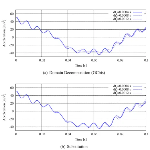
![Figure 1.2: Results comparison for a 2-dimensional wave propagation problem taken from [Boucinha et al., 2013].](https://thumb-eu.123doks.com/thumbv2/123doknet/14658737.739216/42.892.255.634.168.422/figure-results-comparison-dimensional-propagation-problem-taken-boucinha.webp)
+7

Documents relatifs
