HAL Id: hal-01926479
https://hal.archives-ouvertes.fr/hal-01926479
Submitted on 19 Nov 2018HAL is a multi-disciplinary open access archive for the deposit and dissemination of sci-entific research documents, whether they are pub-lished or not. The documents may come from teaching and research institutions in France or abroad, or from public or private research centers.
L’archive ouverte pluridisciplinaire HAL, est destinée au dépôt et à la diffusion de documents scientifiques de niveau recherche, publiés ou non, émanant des établissements d’enseignement et de recherche français ou étrangers, des laboratoires publics ou privés.
Multi model Arlequin Method for fast transient
dynamics in explicit time integration
Alexandre Fernier, Vincent Faucher, Olivier Jamond
To cite this version:
Alexandre Fernier, Vincent Faucher, Olivier Jamond. Multi model Arlequin Method for fast transient dynamics in explicit time integration. 13e colloque national en calcul des structures, Université Paris-Saclay, May 2017, Giens, Var, France. �hal-01926479�
CSMA 2017
13ème Colloque National en Calcul des Structures 15-19 Mai 2017, Presqu’île de Giens (Var)
Multi-model Arlequin method for transient structural
dyna-mics with explicit time integration
A. Fernier1, V. Faucher2, O. Jamond1
1 CEA, DEN, DANS, DM2S, SEMT, DYN, Gif sur Yvette F-91191 2 CEA, DEN, Cadarache, DTN/Dir, F-13108 St Paul lez Durance, France
Résumé — This paper addresses the explicit time integration for solving multi-model structural dynamics by the Arlequin method. Our study focuses on the stability of the central difference scheme in the Arlequin framework. Although the Arlequin coupling matrices can introduce a weak instability, the time integrator remains stable as long as the initial kinematic conditions of both models agree on the coupling zone. After showing that the Arlequin weights have an adverse impact on the critical time step, we present two approaches to circumvent this issue and test them on relevant examples.
Mots clés — Arlequin method, Multi model, Structural dynamics, Explicit time integration, Stability
1
Introduction
The Arlequin method has been developed as a flexible engineering tool [1] allowing the coupling of different models (particle, continuum, SPH) and meshes (1D-2D, 1D-3D) in both statics and dynamics [2], [3], [4]. Moreover, using a partition of unity approach provides a progressive and smooth transition between the different models. Previous studies have found the Arlequin method to be relevant for dynamic simulations, as wave transition is guaranteed and spurious effects can be corrected if the parameters are used adequately [5]. The Arlequin method was also extended to an energy conservative multi-time explicit-implicit method for the Newmark family of time-integrators [6], [7].
In this study, we address the explicit-explicit time integration of the Arlequin formulation for linear structural dynamics. It is very useful when simulating fast transient dynamics, which is the focus of this article.
2
Governing equations of the Arlequin method
2.1 Continuous formulation
We consider an isotropic elastic body occupying a bounded, regular domain Ω1∈ Rd. A local
model, Ω2, is superimposed to the global model, Ω1, in the neighbourhood of a zone of interest. We assume for clarity that Ω2 is strictly embedded in Ω1. Sub-domain Ω2 is partitioned into
two regular, non-overlapping domains : the coupling zone Ωc and the free zone Ωf. Let ui, ˙ui
and ¨ui denote the displacement, velocity, and acceleration fields of model i while u0i and ˙ui0
its initial displacement and velocity. The boundary ∂Ω1 of Ω1 is partitioned into two parts, Γu
and Γh, such that Γu∩ Γh= ∅. The body is submitted to volume forces g ∈ L2(Ω1), prescribed
displacements up on Γu 6= ∅ and prescribed boundary forces h on Γh. Let ρ be the material density, σ the Cauchy stress tensor, and ε the infinitesimal strain tensor. The strain tensor is given by ε = ∇Su = 12(∇u + ∇Tu) while the stress tensor is given by Hooke’s law : σ = D : ε
where D is the elastic tensor.
Given g, h, up, u0 and ˙u0, find (u1(t), u2(t), λ(t)) ∈ V1× V2× M, t ∈ [0, T ] such that ∀ v1∈ V01, m1(u1(t), v1) + k1(u1(t), v1) + c(u1(t), λ(t)) = f1(v1) ∀ v2∈ V2 0, m2(u2(t), v2) + k2(u2(t), v2) − c(u1(t), λ(t)) = f2(v2) ∀ µ ∈ M, c(µ, ¨u1(t) − ¨u2(t)) = 0 (1) with (i=1,2) mi(u(t), v) = d2 dt2 Z Ωi αiρ u(t) · v dΩi ki(u(t), v) = Z Ωi
αi σ(u(t)) : ε(v) dΩi
fi(v) = Z Ωi αi g(t) · v dΩi+ Z Γfi αi h(t) · v dΓfi c(µ, w(t)) = Z Ωc µ · w(t) + L2 ε(µ) : ε(w(t)) dΩc (2) where Vi= {w(t) ∈ H1(Ωi)d | w = up on Γdi} and V i 0= {w ∈ H1(Ωi)d | w = 0 on Γi}. M = {λ ∈ H1(Ωc)d} is called the mediator space, L is a strictly positive parameter homogeneous to a length (typically the thickness of the coupling zone), and w ∈ V = H1(Ωc)d is an acceleration gap field.
The internal energy weight parameter functions αi, i = 1, 2, are defined in the whole domain
Ω1. They are assumed to be independent of time and satisfy :
αi∈ [0, 1] and α1+ α2= 1 in Ω1; α1= 1 in Ω1\Ω2 and ∃α0, αi≥ α0 in Ωf (3)
The constant α0 has to be arbitrarily small for the Arlequin method to be relevant [8].
2.2 Discrete formulation
The finite element discretization of the equations (1)-(3) leads to the following system :
Given initial conditions Ui0 and ˙Ui
0 for i = 1, 2 and ∀n ∈J0, N K M1U¨1n+ K1U1n+ C1Tλn= F1n M2U¨2n+ K2U2n− C2Tλn= F2n C1U¨1 n − C2U¨2 n = 0 (4)
where Mi, Ki are, respectively, the mass and stiffness matrices on sub-domain Ωi. Fi is the load
vector applied on sub-domain Ωi, while CiT and λ are, respectively, the coupling matrix and the Lagrange multiplier vector in the coupling zone Ωc.
This system of equations can be rewritten as a differential algebraic system (DAS) :
M CT C 0 ! " ¨ Un ¨ νn # + K 0 0 0 ! " Un νn # = F n 0 ! (5)
where M = diag(M1, M2), K = diag(K1, K2), C = [C1, −C2], Un= [U1n, U2n]T, Fn= [F1n, F2n]T
and ¨νn= λn.
3
Stability of differential algebraic system
In this study, the central difference scheme is used for time integration. It is known to be conditionally stable under the condition :
∆t < ∆tc= s 2 ω2 max (6)
where ∆tc is the critical time step and ωmax is the maximum eigenfrequency of the generalized eigenvalue problem of K and M . However, this result is only valid for a differential system with the right properties (K is not singular and A = M +14∆t2K is positive definite). For the
differential algebraic system (5), further analysis must be done. It was shown in [9] that the Lagrange multipliers do not have a negative impact on the critical time step as long as C ˙U0= 0 and CU0= 0.
4
Impact of the Arlequin weights on the critical time step
The other component of the Arlequin framework that can affect the stability is the Arlequin weighting. In most industrial codes, instead of computing the maximum eigenfrequency of the global problem to define the critical time step, as in (6), the maximal eigenfrequency on each element is computed. Indeed, [10] states that, assuming that ωE is the highest frequency of thegeneralised eigenvalue problem of KE and ME (for element E), if max ωE2 is substituted to ω2max in the computation of the critical time step (6), then the time-integrator remains stable. Such a computed critical time step is noted ∆Etc and we thus have ∆Etc≤ ∆tc. In this analysis, in
order to study the impact of the weighting on ωE2, we will consider a single element.
4.1 Impact on a single element
It is not always possible to ensure that the Arlequin weights are constant on an element, such as when linear or cubic weight functions are used in the overlapping zone, or when the meshes of different models do not match. In this section, we will consider a one dimensional element in which the Arelquin weight is piecewise constant, as shown in Figure 1.
The goal of this simplified case is to identify the parameters that influence the critical time step and use any relevant conclusions for higher dimension computations. In this scope, the parameter δ represents the location of the weight function discontinuity within the element. It is important to note that when dealing with 2D or 3D meshes that do not match, the position of the discontinuities can not be controlled and, therefore, δ is arbitrary and can take any value in its range. The beam of length L is assumed to be elastic with density ρ and Young modulus
α1
1
δL
α2
0 L
Figure 1 – Model of a 1D elastic beam in which the weight function is piecewise constant.
E so that σ = Eε. The weight function is piecewise constant equal to α1 on [0, δL] and equal to
α2 on [δL, L] where δ ∈ [0, 1] is the previously introduced geometric parameter.
The critical time step was determined using a formal algebra software and is given by (7) :
∆tc= γ(qα, δ)∆tgc (7) with γ(qα, δ) = p q2 α+ 2qα(1 − qα)δ + (1 − qα)2(2δ3− δ4)) qα+ (1 − qα)δ , qα= α2 α1 , ∆tgc= rρ E
where ∆tgc is the critical time step of the unweighed problem.
It is interesting to note that the critical time step depends on only two variables : parameter
δ and the ratio of the two weights qα. As the function has symmetry1, we can consider that 0 < qα< 1. Function γ is plotted in Figure 2.
1. It can be shown that γ(q1
We observe that function γ, and, thus, the critical time step can drop significantly. As δ is arbitrary and can take any value, the critical time step drastically drops when qα is small. In such a case, computations are not feasible. Secondly, we note that if δ = 0, δ = 1, or qα= 1, that
is, if the weight is constant on the element, the critical time step is not altered. We thus propose two approaches to circumvent situations in which the critical time step significantly drops. They are detailed in the next two subsections.
1 0.8 0.6 qα 0.4 0.2 0 0 0.2 0.4 δ 0.6 0.8 1 0.2 0.4 0.6 0.8 1 γ qα 0 0.2 0.4 0.6 0.8 1 β 0 0.1 0.2 0.3 0.4 0.5 0.6 0.7 0.8 0.9 1
Figure 2 – (Left) Evolution of γ, the normalized critical time step, as a function of δ and qα.
(Right) Evolution of β = min
δ γ(δ, qα) for a set qα.
4.2 qα-control approach
We now consider two one dimensional and non conforming meshes coupled through the Arlequin method. In this section, we show how the choice of the coupling zone can ensure a near optimal critical time step.
4.2.1 Limiting qα
We observed in Figure 2 (left) that the critical time step drops when parameter qα is very
small. However, if qα is high enough, the drop in the critical time step is small regardless of
the value of δ. Thus, we numerically determined the value of β = min
δ γ(δ, qα) for a set qα. The
results are shown in Figure 2 (right).
We can see that the highest possible value of β corresponds to a constant weight on the element. Also, for example, we see that qα= 0.5 implies β > 0.985. In other words, if the user ensures that on every element the weight decreases by less than half, then the critical time step will drop by less than 2%, which is acceptable.
In this next subsection we describe how the choice of the coupling zone can ensure that the
qα of any element of any model is always above a minimum value, qmin, which is high enough
that ∆tc is near optimal value. Also, in the following, we distinguish two ’types’ of borders of
the coupling zone, the outer border between in Ωcand Ω1\Ω2 and the inner border between Ωc
and Ωf (see Figure 3).
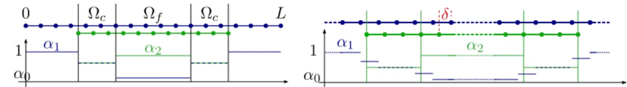
4.2.2 Choice of the coupling zone
Firstly, we propose to use piecewise constant weight functions so that the only elements in which the weights is not constant are the ones crossed by the coupling zone’s borders. These elements are the ones crossed by the vertical lines in Figure 3. Secondly, we set the weights of both models to 12 in Ωc. Now, we will see how such a coupling zone ensures a near optimal critical time step.
We note that according to the previous study, the elements that have a constant weight do not affect stability. Then, with the characteristics described in the previous paragraph, the only
elements that can affect the stability are those crossed by the coupling zone’s border (see Figure 3 (left)).
Let’s first consider the elements crossed by the outer border. It is natural to align the outer border with the mesh of Ω2. In this case, the outer border only crosses elements of the Ω1 (in blue in Figure 3). These elements’ weight now takes two values, 1 and 12 so that qα on that element is equal to 0.5. According to the previous study, the critical time step can only decrease by at most 2% which is acceptable.
Now, let’s consider the inner border. If it is aligned with the mesh of Ω2 then, with the same reasoning as before, only elements of Ω1 are crossed by it, their weight take two values, 12 and α0
so that their qα equals 2α0. As α0 can be arbitrary small and according to the previous study,
the critical time step can drop significantly. On the other hand, if the inner border is aligned with the mesh of Ω1, then only elements of Ω2 are crossed by it and their weight can take two
values, 12 and 1 − α0 so that their qα is greater than 0.5. Thus, with this choice of inner border,
the the critical time step can only decrease by at most 2% which is acceptable. This is the inner border used for the qα-control approach.
It is easy to see that with this reasoning, any other choice of inner border (for example not aligned with either mesh) would imply a significant drop in the critical time step. In the results sections, in order to show the relevance of the qα-control approach, we compare it with a
so-called patch-aligned Ωcapproach in which the inner border is arbitrarily chosen to be aligned
with the mesh of Ω2 (and thus has a critical time step that potentially drops significantly, see previous paragraph). α1 1 0 L α2 α0 Ωc Ωf Ωc α1 1 α2 α0 δ
Figure 3 – Weight functions for the qα-control (left) and the averaged weight (right) approaches.
4.3 Averaged weight approach
As was seen in the previous sections, if the weight on an element is constant then it does not affect the stability. Thus, we propose another approach in which we first define weight functions α for both models. Then, for each element, we average the value of its weight ¯αE=|Ω1E|
R
ΩEα dΩE
where |ΩE| is the volume of element E. We define the averaged weight function ¯α such that
¯
α|E = ¯αE.
This approach maintains an optimal critical time step, is very easy to implement, and ensures that no geometric parameter affects the stability. However, the partition of unity in equations (3) is no longer verified on elements in which the weight would normally vary (see Figure 3 (right)) and a loss in accuracy can be expected. In order to limit the number of elements in which this occurs, we propose to use piecewise constant weight functions (see Figure 3 (right)).
5
A 2D consistency test
5.1 Presentation
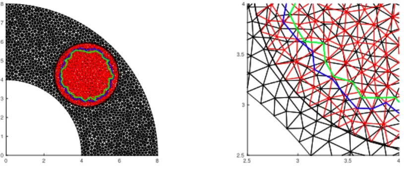
In this section we consider a quarter of a thick-walled tube, as represented in Figure 4. We assume the tube to be made of steel and use plane strain. The horizontal (bottom) and vertical (left) sides of the plate are clamped in their normal direction, but free to move in their tangential direction. A constant, uniform force is applied on the inner side of the plate in the normal direction during a time ∆tF. A circular wave is thus created. It moves outward, then bounces first off the outer circular boundary, then off the inner circular one, etc. The simulation lasts for about ten round trips of the wave. A small, linear damping equal is also implemented.
The mono-model mesh is unstructured, as represented in black in Figure 4. The substra-te’s mesh, Ω1, is identical to the mono-model’s and the patch’s, Ω2, is also unstructured and represented in red in Figure 4.
0 2 4 6 8 0 1 2 3 4 5 6 7 8 2.5 3 3.5 4 2.5 3 3.5 4
Figure 4 – Figure of the meshes and the boundaries of the coupling zone (left), and a zoom on the frontiers (right). The substrate (and mono-model) mesh is in black, and the patch mesh is in red. The blue line represents the inner boundary of the coupling zone for the averaged weights approach, and the green line represents that of the qα-control approach. The outer boundary of
the coupling zone is in black, and is common to both approaches.
5.1.1 Error measurement
In order to evaluate how precise the two approaches are, we compare them to the mono-model solution. To make the comparison, we introduce the following error measurement :
Eu(t) = ||ur(t) − ua(t)||L2(Ω 1) max τ ||u r(τ )|| L2(Ω 1) (8)
where u is the displacement. The subscript0r0 denotes the reference, mono-model solution while
0a0 denotes the Arlequin solution (ua= α
1u1+ α2u2).
5.2 Results
The critical time steps ∆tcand ∆Etcare computed for each approach, including, for relevancy,
the patch-aligned Ωcapproach and compared with the optimal values given by the mono-model computation. The results are shown in Table 1. We see that both critical time steps for the
Monomodel qα-control Averaged weights Patch-aligned ΩC
∆tc 1.813 1.813 1.807 0.728
∆Etc 0.977 0.977 0.977 0.438
Table 1 – Critical time step in 10−5 s for all approaches. Values of ∆Etc always correspond to
an element in the coupling zone (α0= 1.0 × 10⁻⁶).
patch-aligned ΩC approach drop significantly (60% for ∆tcand 55% for ∆Etc). The two proposed
method however, have near optimal values of the critical time steps, confirming their efficiency.
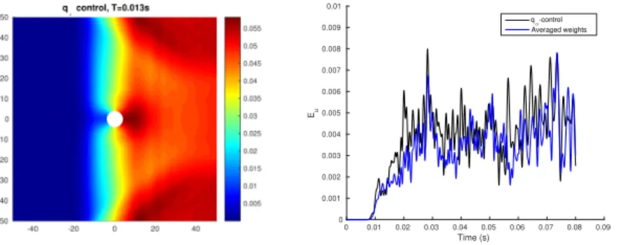
Both the averaged weight and the qα-control approaches were implemented and compared to the mono-model solution (see Figure 5). After ten round trips, the displacements are all very similar and thus only one approach is shown (Figure 5). The error computation using the error measurement (8) confirms good agreement as both Arlequin approaches yield a very small error that steadies around 0.5%, thus validating them.
Time (s) 0 0.002 0.004 0.006 0.008 0.01 0.012 0.014 Eu 0 0.001 0.002 0.003 0.004 0.005 0.006 0.007 0.008 0.009 0.01 qα-control Averaged weights
Figure 5 – (Left) Snapshot of the displacement (in meters) in the tube for the qα-control. The
wave is expanding outward after completing ten round trips. (Right) Error, Eu, as defined by
equation (8), plotted over time for both approaches.
5.3 Geometric discrepancy : a holed plate
In this section, now that the stability results have been validated, we consider the accuracy and the relevance of the Arlequin framework. In order to do that, we introduce an example in which the patch introduces a discrepancy not present in the substrate.
5.3.1 Presentation
In this section we consider a square plate of constant density and Young’s modulus containing a hole and plane stress is used. Let the substrate, Ω1, be a square plate of side length 100m, and let the patch, Ω2, be a web shaped mesh with a hole in it. The outer radius is 20 m, and
the inner one is 4 m. The patch is superimposed in the center of the substrate. The reference mono-model is constructed such that it is identical to the substrate in its outer part and is fairly close to the patch in its center. In Figure 6, we see that the holes from both the mono-model and the Arlequin formulation are fairly similar, reducing the risk of discrepancies due to mesh differences.
The left side of the square plate is clamped on the x (horizontal) axis and free to move on the y (vertical) axis. A constant, uniform force F , is applied on the right side of the plate in the x direction during a time ∆tF. A wave moving left is thus created. It hits the hole and then bounces off the left boundary. The simulations last for about two round trips of the wave. A small linear damping was also implemented.
-50 0 50 -50 -40 -30 -20 -10 0 10 20 30 40 50 -20 -10 0 10 20 -20 -15 -10 -5 0 5 10 15 20 −50 0 50 −50 −40 −30 −20 −10 0 10 20 30 40 50 −5 0 5 −5 −4 −3 −2 −1 0 1 2 3 4 5
Figure 6 – From left to right : 1) Mesh of the substrate (black) and the patch (red) – 2) Zoom on the patch. The outer border of Ωc is black while the inner one is blue (averaged weight approach) or green (qα-control approach) – 3) The mono-model mesh – 4) Comparison of the
meshes of the hole of the mono-model (black) and the Arlequin ones (red).
Error measurement In order to compare the two solutions, the difference in the shape of the hole was evaluated using the same error measurement as in the previous section except that it is solely measured on the hole boundary ∂ΩH.
5.3.2 Results
As in the previous section, the critical time steps ∆tc and ∆Etc were computed for each
Monomodel qα-control Averaged weights Patch-aligned Ωc
∆tc 4.952 6.703 6.703 6.703
∆Etc 4.293 6.016 6.016 6.016
Table 2 – Critical time step in 10−5 s for all approaches.
case, the critical time step is always determined by the elements around the hole, which are a lot smaller than those in the coupling zones. This is why both ∆tc and ∆Etc are the same for the
three Arlequin and patch-aligned approaches. Yet they differ from the mono-model because the meshes are different. It is interesting to note that the values have the same order of magnitude, confirming that the two meshes are fairly similar.
The solutions of the mono-model, the averaged weights, and the qα-control approaches were
implemented to calculate displacement across time (see Figure 7). The error illustrated in Figure 7 confirms that the solutions of the Arlequin models agree. Both approaches yield low error mea-sures. The error seems to steady around 0.5%, and does not exceed 0.8%, once more validating both approaches. Time (s) 0 0.01 0.02 0.03 0.04 0.05 0.06 0.07 0.08 0.09 Eu 0 0.001 0.002 0.003 0.004 0.005 0.006 0.007 0.008 0.009 0.01 qα-control Averaged weights
Figure 7 – (Left) Snapshot of the displacement (in meters) of the plate for the qα-control when
the wave has entered the patch and collides witth the hole. (Right) The Error measurement for both approaches.
Références
[1] H. Ben Dhia and G. Rateau. The arlequin method as a flexible engineering design tool. Numerical
Methods in Engineering, 62(11) :1442–1462, 2005.
[2] P. T. Bauman, H. Ben Dhia, N. Elkhodja, et al. On the application of the arlequin method to the coupling of particles and continuum models. Computational Mechanics, 42 :511–530, 2008.
[3] S. Prudhomme et al. Computational analysis of modeling error for the coupling of particle and continuum models by the arlequin method. Comp. Meth. App. Mech. Eng., pages 3399–3409, 2008. [4] F. Caleyron et al. Sph modeling of fluid/solid interaction for dynamic failure analysis of fluid-filled
thin shells. Journal of Fluids and Structures, 39 :126–153, 2013.
[5] L. Chamoin et al. Ghost forces and spurious effects in atomic-to-continuum coupling methods by the arlequin approach. IJNME, 83 :1081–1113, 2010.
[6] A. Gravouil and A. Combescure. Multi time step explicit-implicit method for non linear structural dynamics. International Journal for Numerical Methods in Engineering, 50(1) :199–225, 2001. [7] A. Ghanem et al. Arlequin framework for multi-model, multi-time scale and heterogeneous time
integrators for structural transient dynamics. Comp. Meth. App. Mech. Eng., 254 :292–308, 2012. [8] H. Ben Dhia. Further insights by theoretical investigations of the multiscale arlequin method.
International Journal for Multiscale Computational Engineering, 6(3) :215–232, 2008.
[9] C. Farhat, L. Crivelli, and M. Geradin. Implicit time integration of a class of constrained hybrid formulations - part 1 : Spectral stability theory. Comp. Meth. App. Mech. Eng., 125 :71–107, 1995. [10] A. Gravouil. Méthode multi-échelles en temps et en espace avec décomposition de domaines pour la