Constraint Modeling for Curves and Surfaces in CAGD: A Survey

HAL Id: hal-00118989

https://hal.archives-ouvertes.fr/hal-00118989

Submitted on 7 Dec 2006

HAL is a multi-disciplinary open access

archive for the deposit and dissemination of sci-entific research documents, whether they are pub-lished or not. The documents may come from teaching and research institutions in France or abroad, or from public or private research centers.

L’archive ouverte pluridisciplinaire HAL, est destinée au dépôt et à la diffusion de documents scientifiques de niveau recherche, publiés ou non, émanant des établissements d’enseignement et de recherche français ou étrangers, des laboratoires publics ou privés.

Constraint Modeling for Curves and Surfaces in CAGD:

A Survey

Vincent Cheutet, Marc Daniel, Stefanie Hahmann, Raphaël La Greca,

Jean-Claude Léon, Robert Maculet, David Ménegaux, Basile Sauvage

To cite this version:

Vincent Cheutet, Marc Daniel, Stefanie Hahmann, Raphaël La Greca, Jean-Claude Léon, et al.. Constraint Modeling for Curves and Surfaces in CAGD: A Survey. International Journal of Shape Modeling, World Scientific Publishing, 2007, 13 (2), pp.159-199. �10.1142/S0218654307000993�. �hal-00118989�

Constraint Modeling for Curves and Surfaces in CAGD:

A Survey

Vincent Cheutet

∗

, Marc Daniel

†

, Stefanie Hahmann

‡

, Rapha¨el La Greca

†

,

Jean-Claude L´eon

§

, Robert Maculet

†

, David M´enegaux

¶

, Basile Sauvage

‡

Abstract

Computer-Aided Geometric Design modelers are now based on powerful mathematical curve and surface models, but there is still a considerable need for efficient tools to handle, analyze and modify these objects. Designing product shapes using geometric operations on free-form curves and surfaces is still a tedious task. Moreover, designers would prefer to use meaningful tools to concentrate on design objectives expressed in terms of functionalities and constraints related to engineering topics and technical matters.

This explains why constraint modeling in CAGD is an important challenge for the forthcoming years and the paper aims at setting up some of its foundations. The corre-sponding global modeling approaches already proposed in CAD are first exposed. The specific existing techniques for handling constraints on curves and surfaces are then sur-veyed. A synthesis of these techniques and our current studies allows us to suggest a classification of the different constraints which ought to be taken into account in a con-straint based modeling CAGD software. Open issues in the context of engineering design are finally emphasized.

1

Introduction

The most important improvements in curve and surface modeling result in the introduction of new mathematical models: B´ezier, B-splines, NURBS, triangular models, subdivision curves and surfaces. The reader unfamiliar with Computer-Aided Geometric Design (CAGD) concepts can refer for example to [30, 56, 110]. These free-form curve and surface models have signifi-cantly increased the quality of the designed objects assuming the ability of the user to handle the different parameters, generally defined in terms of geometry. Improving the ergonomics and efficiency of these design handles in order to manipulate, analyze and modify objects is still a research issue. Moreover, when a designer uses a CAGD software, his/her expectations would be to express and solve the problem as a relevant problem of design. The latter problem to solve is given in terms of functionalities and various types of constraints including geometry,

∗_{IMATI CNR, Genova, Italy (vincent.cheutet@hmg.inpg.fr)}

†_{Laboratoire LSIS, Marseille, France (Firstname.Lastname@esil.univ-mrs.fr)}

‡_{Laboratoire Jean Kuntzmann, INP Grenoble, France (Firstname.Lastname@imag.fr)} §_{Laboratoire 3S, INP Grenoble, France (Firstname.Lastname@hmg.inpg.fr)}

engineering topics, mechanics, manufacturing, know-how, industrial context, economy, ... and is sometimes badly structured, especially at the beginning of the process. This explains why requirements for curve and surface modeling techniques are currently changing and more and more oriented toward a constraint based modeling approach. This new approach will directly lead first to express constraints and then to solve a high number of various constraints. It thus raises a lot of difficult issues while it corresponds to an actual need in industry.

But the industrial requirements for manufactured objects are complex. It may be impossible to model a real shape with a unique surface so that the object must be defined by a set of surfaces connected together through continuity constraints (tangency or curvature). Moreover, even for one surface, the mathematical models currently applied (B-spline or NURBS) cannot always represent the reality and/or the topology of the shape. As a result, the user must define a larger surface and then define a restriction curve on the surface which surrounds its relevant part. The curve, given in the parametric definition plane is called trimmed curve and the relevant surface is called trimmed surface. This approximate operation raises well-known inaccuracies. We point out this particular problem because the different connected surfaces defining an object are most of the time trimmed surfaces.

Figure 1: An example of a motorbike streamliner.

Figure 1 proposes a real example of a motorbike streamliner and its model defined with a trimmed B-spline surface with two holes. The control net defining this B-spline surface is also shown, emphasizing the difficulty of defining the control point locations.

The previous example illustrates that constraint modeling in CAGD is an important chal-lenge for the forthcoming years: this paper aims at setting-up some of its foundations and is organized as follows. Since there are many similarities in the objectives, section 2 presents the global approaches developed in CAD modelers. Section 3 is devoted to a presentation of exist-ing constraint-based modelexist-ing techniques for the most frequent types of curves and surfaces. These specific techniques are generally used during free-form modeling. A synthesis of these prior contributions and our current studies allows us to suggest in section 4 a classification of the different constraints which ought to be taken into account in a constraint-based modeling CAGD software. Open issues in the context of engineering design are finally emphasized at section 5.

2

Modeling approaches in CAD

The expectations stated in the introduction also concern any CAD process and have evidently been studied in this context for simpler objects. Different approaches have been developed and describing them is relevant in our framework: parametric and variational approaches on the one hand and feature-based approaches on the other hand. In addition, the declarative modeling approach can be considered as complementary to the previous ones and located at a higher level. The first distinction which can be made between these different approaches is the level of abstraction used to manipulate a model, as suggested by R. Maculet and M. Daniel in [74]:

• Level 0: manipulation of variables, or parameters (e.g.: a point is defined by two param-eters (x, y) in 2D, three (x, y, z) in 3D...).

• Level 1: manipulation of elementary geometric objects (points, straight lines, curves, surfaces); it corresponds to the parametric and variational modelers solving elementary geometric constraints (e.g.: distance between two points, angle between two lines, etc.). • Level 2: manipulation of more complex geometric objects, made up of simple elements

of level 1 associated together (e.g.: groove in an area of an object); it corresponds to the feature-based approach, to solve more complex constraints (e.g.: length of the groove), and which are generally associated with a semantic meaning or with geometric properties.

The second point used to differentiate modelers is the concept of directed constraint and undirected constraint. For example, let a rectangle be of length L and width l. A directed constraint would be: L = 2 × l. The width l is initially known, then L can be evaluated with this directed constraint. On the other hand, an undirected constraint would be: L − (2 × l) = 0. In this case, L or l can be modified indifferently.

The third difference among the modeling approaches holds in the fact that either purely geometric constraints or constraints incorporating non-geometrical parameters (like engineer-ing constraints) can be expressed. Here, engineerengineer-ing constraints designate more specifically equations containing geometric parameters of the product as well as technological, mechanical parameters (forces, power, stresses, ...).

Several approaches exist at present to meet the needs of the designer, depending on the desired level of abstraction considered to manipulate an object. The next subsections are an attempt to decompose these different approaches, which could be structured this way: para-metric and variational approaches on the one hand and, on the other hand, featured-based and declarative approaches.

2.1

The parametric modeling approach

This approach considers elements from the first two levels, manipulating only directed con-straints. From an object given by a geometrical configuration, the same object can be defined and obtained by specifying parameters (or variables). The parameter settings are dimensional and functional.

This approach is sequential as it allows the modification of a model by changing instan-tiations of its constitutive geometric objects, given in a prescribed order. For example, a parametric modeler can build a triangle defined by two edges and an angle (see Figure 2, left).

Figure 2: Left: building a triangle defined by two distances dAB and dAC, and an angle α. Right: the problem is cyclic considering simultaneously the distances dAC and dBC.

The generation process is performed sequentially: point A is positioned, then the horizontal straight line is plotted with point B placed at distance dAB; then the straight line which forms an angle α with dAB is plotted and finally point C is placed at a distance dAC. On the other hand, the next example of a triangle given by the lengths of the three edges only cannot be solved sequentially. In this case, the distances dAC and dBC must be considered together to solve the problem (see Figure 2, right). They are two coupled constraints and the problem is known as cyclic. A variational approach is thus necessary (see section 2.2) to obtain a solution. A problem is said to be parametric if it can be divided into a set of subproblems that can be sequentially solved one after the other [55]. There is thus a history for the sequence of construction that should be re-expanded each time the model receives modifications. Since it is not possible to solve a general problem and to place objects simultaneously, there are limitations on the constraints that can be considered in this approach. The explicit constraints, in which all the parameters can be extracted, are used to generate a solution.

The limits of this modeling approach rely on its constraint resolution simplicity. There is no possible coupling between the geometric constraints and the engineering ones [20]. Each step of the solving process takes into account only one constraint involving geometric objects: this constraint is at ”level 1” and corresponds to a subsystem of equations at the level of variables (”level 0”). The constraints should not:

• be cyclic as for example in the last case of construction of the triangle for which only the lengths of the three edges are known,

• correspond to constructions ”with a ruler and a compass” [64]. They are irreducible subsystems.

This approach gives only one solution if it exists and is unable to obtain multiple solutions. The user has only access to a predetermined set of parameters, that he/she should implement in a predefined order, reducing the flexibility of the design process. From a complementary point of view, if one parameter is not adapted or out of its domain of validity, the sequence of operations can give an idea of the influence of each parameter whereas this may be more complex with the next category of approaches.

The set of expressed constraints must imperatively be iso-constrained. However, during the design process, this set is generally under-constrained and sometimes over-constrained because it is difficult for the designer to make sure that all the constraints stay consistent with respect to each other and that the number of inserted variables is adequate to correctly describe the variations of the designed product. The set of constraints becomes iso-constrained after the designer has carefully analyzed the product variations he/she desires. Thus, the variational approach has been developed to give a better answer to the designer’s needs.

2.2

The variational modeling approach

The designation of variational geometry first appeared in CAD with Lin, Gossard and Light [65]. This approach is a completely declarative approach considering solely entities from the first two levels.

Hoffmannand Joan-Arinyo stated in [55] that a problem is known as variational if it can be divided into several subproblems which are simultaneously solvable as systems of constraints. The constraints can be at the same time geometrical but also of engineering type. However, these last ones are often equations containing geometric and non-geometric parameters of the object: it generally induces a strong coupling between these two types of constraints.

According to the configuration of the problem (under-/iso-/over-constrained, see section 4.5), the solver is able to find a correct set of solutions. In configurations where no solution is found, two possibilities arise: the problem is either over-constrained or has no solution (with the corresponding set of values). Several decomposition methods have been developed to supple-ment the solving methods and help the designer when under-/over-constrained configurations are encountered.

This global resolution of a set of constraints is rather complex. The complexity of the reso-lution and the computation time grow as the number of geometric objects becomes larger. Most variational modelers are in 2D as opposed to parametric modelers that can handle 3D configu-rations. These variational modelers are called sketchers since the designer works interactively with the CAD systems, and generates his/her preliminary design.

2.3

The feature-based modeling approach

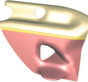
This approach considers entities from level two, called features (or characteristics) which can be of several types, and particularly of form feature type for characterizing the shape of a compo-nent. In addition, complementary entities were integrated into the previous model, making it possible to characterize some operations of the manufacturing process or other designer knowl-edge at other stages of the design process. The issue of this approach is to directly manipulate the shape of a component and the semantics attached to it and no longer the intrinsic definition of the geometric entities of this component. These entities are complex sets of simple elements: for example, the feature ”hole” is composed by a set of cylinders and planes attached to an initial plane. The extension of features to the free-form domain has been a well-known problem for fifteen years. As an example, the shape of the motorbike streamliner (see Figure 1) can be designed with a feature-based approach, with for instance a feature hole for the cooling system opening and a feature bump for the fin (see Figure 3).

A classification has been proposed by Fontana [33] and extended by Pernot [85]. Four levels have been proposed, from a low level of shape control toward higher possibilities (see Figure 4):

Figure 3: The motorbike streamliner designed by features.

• Form Features: are only composed of primitive surfaces, like planes or cylinders. Some form features are available in the current CAD modelers, like the feature ”hole”.

• Semi Free-Form Features: defined by free-form surfaces, are obtained by classical surface generation rules such as sweep or loft operations, interpolation rules or specific relation-ships directly expressed between control points. The free-form surfaces are thus totally defined by a restrictive set of parameters, the ones of the generative operations.

• Free-Form Features: are obtained through the use of shape change techniques, often based on deformation techniques, expressing a homogeneous behavior over the whole surface. More freedom in defining a complex shape is obtained but monitoring the modified area is not always as free as needed.

• Fully Free-Form Features: are characterized by a higher level of freedom in the shape definition obtained through the use of techniques prescribing heterogeneous behaviors over different areas of free-form surfaces. Such entities fit well the stylists’ requirements.

The feature-based approach can derive from the parametric approach (a set of predefined parameters completely defines the intrinsic dimension of the features, and its position on the product) or from the variational approach (a set of equations/constraints defines it).

The first works about this subject are from Shah [102] and Marks [76]. There are two types of feature-based approaches [103]: the procedural approach that is similar to the para-metric approach with regard to the resolution process, and the declarative approach similar to the variational approach. But the majority of the industrial CAD systems based on feature-based modeling approaches are parametric. Therefore, they are procedural and depend on the sequence for generating these features.

In the domain of free-form surfaces, the feature-based and variational modeling approaches are not yet well established. Due to the complexity of these shapes, it is first complex to find the right set of parameters for describing a free-form shape according to the attached semantics and the user’s context. Secondly, the translation of these parameters into constraints for the shape geometry is a difficult step, especially because the number and the type of parameters

Figure 4: Features classification based on the level of shape control.

are not adapted to the number and the location of the degrees of freedom of the underlying surface geometric model.

One way to easily create and manipulate free-form features is to submit a free-form deforma-tion process to constraints [86]: a set of constraints is applied to the surface and the deformadeforma-tion process is combined with a functional to choose one solution. In this case, the parameters of a free-form feature are directly linked to the parameters of the deformation process.

2.4

The declarative approach

The declarative approach can be seen as an extension of the feature-based one, although there is no historical link between them. The level of abstraction is higher there, because the declarative approach is placed on the level of conceptual or semantic modeling (”level 3”) [70].

The goal of declarative modeling is to allow the user to create digital model of a physical object by giving only a set of properties about it. The computer builds one, some or all the solutions corresponding to the user’s description. The designer is thus released from calcula-tions and can concentrate on the creation phase. This approach is devoted to quickly make sketches or outlines of the shape of the object. The detailed design is a priori easier with a classical modeler. Since all the object properties have been given, having both a geomet-ric and a semantic descriptions is possible. The object model can be geomet-richer, but maintaining the coherency between the semantic model and the geometric model through the forthcoming designer’s geometric modification is an open challenge.

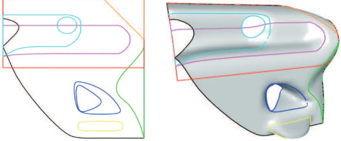
Different applications with this approach have been proposed: polyhedrons [77], space con-trol [15], scene modeling in image synthesis [38, 39, 91]. In the context of this paper, research have been achieved on curves [24, 25], and surfaces [61, 62]. The example proposed in Figure 1 is extracted from this last reference. Figure 5 shows the bording lines on the zones where the different constraints must be applied (left, on the parametric domain, and right, on the

resulting surface): trimming constraints or soft constraints (see section 4.3). Even if interesting results are obtained, they just correspond to the premises of an operational system.

Figure 5: Limits of zones to model the motorbike streamliner: left, in the parametric domain; right, on the surface.

A global system of declarative modeling must include several tools [69]:

• For the description step, in which the conceptual model is clarified in a declarative man-ner, and is refined by a loop of design/re-design. Several methods of description exist: introduction of fuzzy logic in declarative modeling [27], use of a natural or pseudo-natural language [25, 61], sketch and diagram in 2D for the preliminary design [93], etc.

• For the generation step, in which the resolution of a constraint system results from the properties stated during the description.

• A tool allowing the user to browse the set of solutions and enabling him/her to choose one or more solutions and to go on through the loop of design/re-design.

3

Constraint-based free-form modeling techniques

This section surveys the state-of-the-art of constraint-based modeling and/or deformation tech-niques for free-form curves, surfaces and solids. Because of the CAD/CAM background of the present paper, we more focus on NURBS-based representations than on subdivision sur-faces, implicit surfaces or meshes, which are more attractive for computer graphics applications. Indeed, this section is structured in accordance with all these different curve/surface/solid rep-resentations. For each type of representation, the different constraints and constraint-based modeling techniques are addressed. Even if many interesting works have been proposed, the results do not reach all the expectations expressed in the introduction and detailed in section 4.

3.1

Free-form parametric curves and surfaces

The complete theory of parametric free-form curve and surface representations such as NURBS curves and tensor product surfaces, triangular B´ezier patches, n-sided patches, but also Coons

and Gregory surfaces is covered in textbooks by Farin [30], Hoschek and Lasser [56]. Controlling the shape of such geometric objects is often difficult. The modification of control points gives an indication of the resulting deformation, but being extraneous to the object, the control points do not allow for its precise shape control. Limited by the expertise and patience of the user, the direct use of control points as manipulation handles necessitates an explicit specification of a shape deformation process. In addition, large deformations can be extremely difficult to achieve because it is mandatory to move interactively a huge number of individual control points, and the precise modification of the underlying free-form object becomes very tedious. Deformation tools based on geometric constraints offer a more direct control over the shape of curves or surfaces.

3.1.1 Interactive curve and surface modeling

Rather than manipulating control points, picking any point on a B-spline curve or surface and changing its location allows for more direct control of its shape [3, 41, 117]. In [37] Fowler and Bartelscontrol the shape of a B-spline curve by enforcing prescribed geometric constraints, such as the position of a curve point, tangent direction and magnitude, or curvature magnitude. An extension to tensor product B-spline surfaces is given in [36]. This satisfies the user-defined position of surface points, normal direction, tangent plane rotation (to provide a twisting effect), and the first partial derivative magnitude (to generate a tension effect). Borel and Rappoport [10] deform B-spline surfaces by determining the displacement and radius of influence for each constrained surface point. Hsu et al. [57] propose points picking for free-form deformations. Curve constraints, i.e. enforcing the surface to contain a given curve or to model a character line, have been considered in [14, 47, 88].

Adding degrees of freedom to a free-form surface is usually achieved by inserting new vertices into the control polyhedron of a shape, an action that affects either an entire row or column in the control polyhedron of this surface, and hence which is not really a local refinement process. In contrast, hierarchical surface models [35, 44, 122] allow the user to locally adapt a small region of the surface to insert a new detail in the shape.

Free-form feature modeling [12, 34, 111, 112] is a semantic-based approach for shape design and shape control. In contrast to the feature-based approach [78, 98] adopted by CAD systems for classical mechanical design, free-form features are strongly related to aesthetic or styling aspects when modeling with free-form surfaces. This field of application is in fact highly demanding in terms of interactivity to fit with the designer’s way of work.

Surface pasting is a free-form feature modeling technique that composes surfaces to construct surfaces with varying levels of detail. A feature is placed on top of an existing surface to provide a region of increased detail. In [2] B-spline surfaces, called features, are applied to any number of B-spline surfaces, called base surface, in order to add details on the base surface. Improvements and further developments of pasting techniques for B-spline surfaces can be found in [22, 75].

3.1.2 Variational modeling

The variational design paradigm, which has no connection with the approach described in section 2.2, is used in order to find the ”best” curve or surface among all solutions that meet the constraints. These constraints may result from the particular modeling techniques used, like the direct manipulation for example, see section 3.1.1. In the context of smooth curve

and surface design, the notion of ”best” solution is strongly related to the minimization of some functional expressing some energy attached to a curve or a surface, which is called ”soft constraint” at section 4.3.

Although it is difficult to exactly define, in mathematical terms, what fairness of a curve or surface is, it is commonly accepted that smooth and graceful shapes are obtained by minimizing the amount of some energy distributed over the curve or surface. The strain energy functionals originating from elasticity theory are in general non-linear, such as the bending energy for curvesR κ2

(t)dt or the thin-plate energy for surfacesR κ2

1+ κ

2

2dA. These and other higher order

non-linear energy functionals have been used in [46, 83]. In order to accelerate computations, linearized versions of these energy functionals are generally used. For example, Welch et al. [117] maintains the prescribed constraints while calculating a surface as smooth as possible. Celniker and Welch [14] derive interactive sculpting techniques for B-spline surfaces based on energy minimization, keeping some linear geometric surface-constrained features unchanged. Celniker and Gossard [13] enforce linear geometric constraints for shape design using finite elements governed by some surface energy. Historically, the use of such energy functionals goes back to early spline and CAGD literature [81, 95] and has led to a research area, today called Variational Design of smooth curves and surfaces [9, 31, 48, 49, 50].

3.2

Free-form solid modeling

Traditional solid modeling approaches include implicit functions (CSG and blobby models), boundary representations and cell decompositions. The history of solid modeling goes back to the 1980s when the term ”solid modeling” was introduced, see survey papers [96, 97].

Free-form solid models have been pioneered by Sederberg and Parry [101]. They developed a technique for globally deforming solid models in a free-form manner, called free-form deforma-tion (FFD). The three-dimensional object to be deformed is embedded in a three-dimensional parametric space, called the control lattice. The control vertices of the object’s surface are assigned parametric values that depend on their positions inside the parametric solid (usually a B´ezier or B-spline solid) used to monitor the deformation process. As a result, a deformation applied to this solid via its control points deforms the embedded object as the answer to the user’s input. FFD lattices can be patches connected together to provide local control over the deformation area. Coquillart [23] extended FFD to non-parallelepipedal lattices, represented by rational splines. Hsu et al. [57] improved the traditional FFD with a technique that allows the user to manipulate directly the embedded object. It computes how the B´ezier (or B-spline) control points must move in order to produce the desired deformation. Shi-Min et al. [104] proposed a similar scheme in which the computation of a FFD function is based on the ma-nipulation and translation of a single point. Complex deformations are then achieved via the composition of several such single-point FFDs. MacCracken and Joy[73] generalized FFD by incorporating arbitrary-topology subdivision-based lattices.

The use of constraints has mainly been developed from interaction with free-form solids. Rappoport et al. [94] derived a method for modeling trivariate B´ezier solids while preserving the volumes. Different solids can be patched together at their boundaries to create a more complex object. Their algorithm uses an energy minimization function whose purpose is to preserve the volume during sculpting. In addition to the volume-preserving constraint, their system can satisfy interpatch continuity constraints, positional constraints, attachment constraints, and inter-point constraints.

Hirota et al. [54] developed an algorithm for preserving the global volume of a B-rep solid undergoing a free-form deformation. Following a user-specified deformation, the algorithm com-putes the new node positions of the deformation lattice while minimizing an energy functional subjected to the volume preservation constraint. During initialization, each triangle in the sur-face is projected onto the x − y plane, and the volume under the triangle is stored. During the deformation process, this volume is constantly re-computed and compared to the original one. By taking the difference between the volumes of the original and deformed volume elements, the total change in volume is computed.

The FFD process does not check the introduction of surface singularities. Self-intersection could clearly occur. Local self-intersection can be identified via the vanishing Jacobian of the FFD, an approach proposed in [40].

3.3

Multiresolution curves and surfaces modeling

Multiresolution analysis has received considerable attention in recent years in many fields of geometric modeling, computer graphics, and visualization [105]. It provides a powerful tool for efficiently representing functions at multiple Levels-Of-Detail (LOD) with many inherent advantages, including compression, LOD display, progressive transmission and LOD editing. In the literature the term multiresolution (MR) is employed in different contexts, including wavelets, subdivision and hierarchies or multigrids. Multiresolution representations based on wavelets have been developed for parametric curves [19, 32, 71], and can be generalized to tensor-product surfaces, to surfaces of arbitrary topological type [68], to spherical data [100], and to volume data [21].

In the context of free-form geometric modeling, LOD editing allows the modification of the overall shape of a geometric model at any scale while automatically preserving all fine details. In contrast to classical control-point-based editing methods where complex detail-preserving deformations need to manipulate a lot of control points (see sections 4.2, 3.1), MR methods can achieve the same effect by manipulating only a few control points of some low resolution representation. MR manipulation of spline curves and surfaces draws from the ability to project geometry in space Si onto another subspace Si+1 ⊂ Si. Spline spaces are solely defined by the

knot sequences (and the orders). In [19, 71], wavelet decomposition of spline spaces, both uniform and non-uniform are presented. Subspaces are typically selected by removing knots of the knot sequence. While local support is considered the major advantage of the B-spline representations, it is also its Achilles heel. Global modifications are no longer possible on a highly refined B-spline curve. Recognizing this deficiency, in [32, 45], wavelet decomposition was proposed for uniform B-spline curves toward interactive and intuitive MR editing of free-form shapes, see Figures 6 and 7. In [58] direct manipulation of non-unifree-form MR B-spline curves and surfaces is presented.

Figure 6: Multiresolution analysis of quadratic uniform B-spline curve. From left to right the initial curve with 512 control points, and the control polygons of its seven coarse approximations (each having 2i

Figure 7: Multiresolution editing. The hedgehog data (left) set has been deformed at the coars-est level by displacing one of the coarse control points. The deformed coarse polygon is then reconstructed and results in a deformed curve while preserving all the fine details (right).

However, there are application areas, including CAGD and computer animation, where de-formations under constraints are needed. As stated in previous sections, it is obvious that constraints offer an additional and finer control of the deformation applied to curves and sur-faces. In particular, this is important for MR curves and surfaces whose manipulation can be imprecise. Linear constraints include positional constraints, tangential and normal constraints and symmetry, see section 4.2.1. Being linear they are efficiently solved allowing for interactive manipulation. In [29] linear constraints are solved for MR non-uniform B-splines. Non-linear constraints in MR modeling includes area, length and volume prescription. Similar to linear constraints, the preservation of the area enclosed by a planar closed curve or the volume enclosed by a surface can also be solved with small effort because these constraints can be represented as a bi-/tri-linear constraint, see section 4.2.4. Area and length preserving deformations of MR B-splines can be found in [29, 53, 99].

3.4

Implicit surfaces modeling

Implicit surfaces have sparked great interest in the computer graphics and animation community [8, 26, 118, 120, 121], with applications for geometric modeling and scientific visualization [67]. Deformations of implicit surfaces can be obtained intuitively by articulating the skeleton or by changing the parameters of implicit primitives that hierarchically define the surface. Another, more intricate way to deform implicit models is to change the iso-surface progressively by modifying the sample field function defining it.

Two kinds of constraints are particularly easy to integrate. First, collision detection can be accelerated, since in-out functions are provided. Second, implicit surfaces provide a good tool for physics-based animation [26, 121]. Herein well-established laws of physics aim at producing smooth and natural motions in order to create realistic-looking computer animations. To synthesize convincing motions, the animator must specify the variables at each instant in time, while also satisfying kinematic constraints. Deformations of objects are obtained by applying external forces. Gravitational, spring, viscous and collision forces applied to the geometric model act as constraints when deforming the object. Different dynamic behavior of deformable objects have been developed by many varying the imposed constraints, the numerical solution method or by applying these to different geometric models [13, 26, 92, 107, 108, 109, 119, 121]. The volume of an implicit object is another constraint that is important to preserve during deformation [26]. For example, constant volume deformations in a morphing process can make virtual objects look like real ones. A more complete overview on implicit surface modeling can be found in [7].

3.5

Subdivision surface modeling

A subdivision surface is the limit surface of the progressive refinement of a coarse polyhedron, obtained by computing in each step new vertices and joining them up with edges to form a new polyhedron. Subdivision surfaces have become a popular tool in computer graphics in recent years, see [114, 123] for an overview. Different levels of subdivision of a coarse mesh provide different levels of resolution. Constrained modeling techniques can then interact with different subdivision levels in order to obtain particular local design effects.

MacCracken and Joy [73] developed an extension of Catmull-Clark subdivision surfaces to volume setting, mainly for the purpose of free-form deformation in 3D space. Qin et al. [92] introduced dynamic Catmull-Clark subdivision surfaces. McDonnell and Qin [79] simulate volumetric subdivision objects using a mass-spring model. A generalization of McDonnell et al. [80] includes haptic interaction. Capell et al. [11] use the subdivision hierarchies to construct a hierarchical basis to represent displacements of a solid model for dynamic deformations. Additionally, some linear constraints, such as point displacements can be added at any level of subdivision.

Variational subdivision is another modeling technique, where constraints are combined with classical subdivision. Instead of applying explicit rules for the new vertices, Kobbelt’s [59] variational subdivision scheme computes the new vertices such that a fairness functional is minimized. At each step, a linear system has to be solved. The resulting curves have minimal total curvature. Furthermore, in [60] it is shown how wavelets can be constructed by using the Lifting Scheme [106] which are appropriate for variational subdivision curves. Weimer and Warren[113, 115, 116] developed variational subdivision schemes that satisfy partial differential equations, for instance, fluid or thin-plate equations.

Several constrained modeling techniques have been developed by Zorin, Biermann and co-workers for multiresolution subdivision surfaces. A cut-and-paste editing technique for mul-tiresolution surfaces has been proposed in [5]. In [6], Biermann et al. describe a method for creating sharp features and trim regions on multiresolution subdivision surfaces along a set of user-defined curves. A method for approximating results of boolean operations (union, inter-section, difference) applied to free-form solids bounded by multiresolution subdivision surfaces can be found in [4].

4

Classifying constraints for curve and surface modeling

The previous section surveyed different types of constraints allowing the user to handle a shape, from low-level geometric entities to high-level ones, using different concepts for curve, surface, and volume descriptions. The combination of these shape descriptions and constraints covers a subset of the user’s needs. This section proposes a first synthesis of the constraints listed in the previous section as well as a structure of these constraints which must be incorporated to develop a fully constraint-based modeler for curves and surfaces.

4.1

Constraint expression

One of the main difficulties in shape generation and modification is the expression of the user’s intents and their translation into a set of constraints compatible with the chosen geometric

model and the software modeling environment. Three aspects increase the complexity for expressing constraints:

• The first one is to take into account the user’s background or the user’s skills: he/she can be either a stylist, a designer, a manufacturer, etc. Each of these users has a different point of view on the product and its shape. The users express different types of constraints about product modifications during the product development process. These constraints contribute to a so-called product view defined from the appropriate information: product shape, mechanical, technological, ...

• At the same time, the expression of constraints depends of the type of software application used. Their expression can differ when using a CAD modeler or a Virtual Environment with haptic devices. In the first case, the constraints will be directly attached to the model geometry. In the second one, some of the constraints could be expressed in terms of forces to fit capabilities of haptic devices.

• Expressing the constraints is related to the underlying geometric model of a component: a constraint will be differently written if the geometric model is a parametric surface or a surface mesh. Moreover, the difficulty in specifying constraints is increasing when the geometric model type is not uniform over the whole product. Some areas can for instance be described by NURBS surfaces and others by surface meshes. It can also happen that the geometric model of the constraining entity is different from the one of the constrained entity, like a surface mesh constrained by a B-spline curve. These configurations correspond to hybrid models, and are a priori unusual in a CAD modeler. But considering an industrial product through its set of components with all their possible geometric representations can lead to such cases.

From a complementary point of view, the constraints may be related to the product itself rather than to its geometry. It adds the difficulty of formulating constraints that have a meaning at the product level, while incorporating some geometric parameters (e.g. as available in the CAD modelers). Here are two examples of these high level constraints:

• For a manufacturer, one component of the product can be designed to be moulded, and in this case, this component must be extractable from its mould. This high-level constraint (at the product level) can be decomposed into low-level constraints where some of them can be attached to the component geometry by constraining the draft angle of some areas on the surface with respect to the parting plane of the component.

• For a designer, a component of the product should not break during product use. However, this constraint only incorporates mechanical quantities like the maximum stress into the component. Since it needs the strength of the component material and the boundary conditions on the component, this constraint cannot be directly decomposed into lower level constraints referring to the component geometry. Only a Finite Element Analysis (FEA) or similar mechanical analysis methods can provide the proper parameters for this constraint. The FEA cannot be easily incorporated inside a CAD modeler and the extraction of constraints attached to the component shape becomes even more complex. As described, the notion of constraints during a design phase can be very large. This notion is commonly used at all of its successive steps, even if some users don’t bear in mind the

same meaning for these design constraints. We first propose in the following a taxonomy of the constraints classically used for curve and surface modeling and secondly, the various ways a user can express these constraints. Four semantic levels exist for these constraints in the context of shape generation and modification, according to the type of the constrained entity: • Semantic level 1: constraints attached to one element of the component shape: this

in-cludes some local constraints used to manipulate its shape like the point constraints. • Semantic level 2: constraints expressed between two or more geometric elements of the

component shape: for instance, to preserve the integrity of the geometric model of the component during the modification of its shape, like the continuity of its shape.

• Semantic level 3: constraints attached to the whole component shape like a volume con-straint, for example.

• Semantic level 4: constraints not only attached to the component shape but linking its geometry with other parameters of the component, i.e. parameters not directly expressing geometric constraints like functional or engineering ones as illustrated above.

The user first specifies a constraint of any given category. In order to handle it in a second time, a geometric modeler can need to decompose this constraint into a set of constraints of complementary categories (see an example in section 4.2.2). But this decomposition cannot be always achieved and the modeler must be able to handle constraints of different categories at the same time. Moreover, the decomposition is not unique and each modeler has its own way to perform the decomposition.

Then, according to the different approaches described in section 2, two ways of specifying constraints can be proposed that cover all the semantic levels described previously:

• Strict constraints: which are named classically constraints in the literature. The modeler has to strictly respect them during the shape creation and manipulation processes. As an example, the current sketchers in CAD modelers are only using this type of constraints. • Soft constraints: these constraints are used in the declarative modeling approach to allow

the description of the object properties, but also to describe free-form surfaces in the other approaches. They can express the final aspect of a component shape or at least, the expectation to obtain a solution close to it.

The above analysis highlights the complexity of expressing the constraints attached to a product. In the next subsections, the constraints classically used for curve and surface modeling are described in more details, according to the categories previously defined in this section.

4.2

Strict geometric constraints

This section describes the strict constraints commonly used in shape modeling and part of the first two categories previously listed (constraint attached to one geometric element or between two or more geometric elements of a component). Because they are directly related to geometric parameters, the literature named them as geometric constraints. Structuring them requires three complementary concepts:

constrained entity

curve surface constraining entity

point point constraint point constraint shape matching, curve constraint curve

symmetry (character line, ...) shape matching, symmetry, surface projection

connection, ...

Table 1: Constraints with a geometric entity as reference (direct constraints).

constrained entity curve surface

global length, area,... area, volume, inertia, ... tangent plane, local tangent, curvature, ...

principal curvatures, ..

Table 2: Constraints without a geometric entity as reference (indirect constraints).

• The constrained entity: either a curve or a surface.

• The constraining entity: either a point, a curve or a surface.

• Global or local effects, according to the size of the area on which they have a direct influence. Global designates configurations where the entire entity considered is modified. Local means that only an arbitrary subset of the entity is subjected to shape changes. Using these three concepts, Tables 1 and 2 can be considered to classify these constraints. When the constrained entities and the constraining ones have a manifold dimension superior to 0 (i.e. are a curve or a surface), these constraints can require an approximation process and hence are generally decomposed into a set of point constraints. This situation often arises when specifying continuity constraints across several geometric elements of a component. Actually, the continuity conditions across trimmed patches cannot be correctly expressed using the real geometric entities describing the corresponding surface or volume ([30]).

As a consequence, some of the constraints can be structured in a hierarchical manner: an upper level constraint is translated into a set of lower level constraint elements and so forth until receiving a set of point constraints if this elementary type of constraints is the only common denominator to express the desired constraint.

4.2.1 Local constraints

Local geometric constraints are used to locally control a shape, i.e. over a subset of the geometric elements describing the overall shape. The control is achieved through a set of point constraints like position constraints, tangent and normal constraints, curvature constraints, etc. These

constraints correspond to the first line of Table 1, i.e. where the constraining entity is a point. But they also correspond to the second line of Table 2, i.e. with a local effect on the shape.

These constraints provide an ideal tool for direct shape manipulation (see also section 3.1.1). The designer picks a point on a curve or a surface and moves it. It remains to enforce the curve/surface to pass through a new user-specified location using the properties of the under-lying geometric model of curve/surface (see Figure 8). Repeating this operation with small displacement steps leads to a curve/surface select-and-drag tool which continuously deforms the curve/surface. Virtual sculpting techniques make use of this type of constraints.

These constraints are also the most basic constraints, when the decomposition of constraints is required as stated above.

Figure 8: Point and line constraints on the streamliner model.

Let P be a point of the curve/surface, Pu (resp. Pv) be the first derivative vector of the

curve/surface in the u (resp. v) direction at the point considered. Each local constraint can be written as follows:

• Position: −−→P M = ~0, where M can be either a 3D point prescribed by the user or a point of another curve/surface.

• Tangent: −P→u. ~D= 0,

−→

Pv. ~D= 0 (the last one only exists in case of a surface), where ~D can

be either a vector prescribed by the user or the normal vector of another curve/surface. According to the type of curve/surface considered, the derivative −P→u can be different if the type

of curve/surface is no longer parametric but implicit, subdivision, etc. It is also important to note that the position constraint is defined by one vector constraint and so corresponds to three scalar constraints, and the tangent constraint is defined by two scalar constraints.

Position, tangent and normal directions are linear constraints and can efficiently be solved with appropriate methods depending on the underlying geometric model:

• NURBS: methods enumerate as follows ; specification of an area of influence, least-squares fitting with linear constraints (SVD, QR factorization [42]).

• Particular surface models that give direct access to these quantities: interpolating spline curves (position, tangent, curvature), triangular interpolating surfaces (position, tangent, normal) [51, 52, 66, 89, 90, 122].

4.2.2 Curve constraints on a surface

These constraints enforce the surface to match a given curve, in a context of shape modification (see Table 1). One of the current applications is for car aesthetic design: the product is described by a set of curves at some stage of the product specification and this set can be seen as the framework of the product shape model. These curves correspond not only to the object profiles, symmetry lines and selected sections but also to significant lines strongly affecting the product shape, the character lines. Thus, the surface model of the product is directed by these curves [16]. In such a context, the stylists are manipulating a product shape, i.e. its surfaces, through the prescription of curves meaningful for them. Therefore the surfaces have to be constrained by these reference curves.

In the case of continuous surfaces like NURBS surfaces, these curve constraints are, most of the time, decomposed into a set of point constraints, with additional parameters related to the application domain (see Figure 8). This discretization process has a strong influence on the resulting shape. This points out a very complex problem: the curve discretization must not only be too coarse to lose some meaningful variations of the initial curve but must also take into account the distribution of the degrees of freedom over the initial surface to avoid as a result over-constrained configurations. For the specific case of NURBS surfaces, the decomposition is not necessary when the constraining curve can be directly matched with an iso-parametric curve of the surface [82]. However, this case is a very particular one, and is not often encountered in industrial configurations.

When the underlying surface is defined as a mesh, the constraint decomposition process is mandatory since the surface model is a discrete geometric model.

If a curve is constrained by a surface, with a projection constraint for instance, the defined constraint is exactly the same as the curve constraint described at the beginning of this section. The surface is then the constraining element and therefore is not modified during the solving process.

4.2.3 Entity constraints on entities of the same dimension

This section addresses either constraints used to express intrinsic relationships between geo-metric elements of a product (from the second semantic level, as described in section 4.1), i.e. continuity conditions between curves/patches, or constraints related to shape matching con-figurations, from the first semantic level (see Table 1). Shape matching constraints refer to configurations where a geometric entity, e.g. a curve, has to match the shape of a ”reference” geometric entity, e.g. an arc of circle. In the case of continuity conditions, as in Figure 9, the shape can be defined by a set of three B-spline patches and the continuity conditions in position, tangency and/or curvature between them have to be taken into account to preserve the model integrity during the shape transformation.

Considering the geometric continuity conditions, if the constrained geometric elements are trimmed patches, which is the most common case, the constraints need to be decomposed once more. Firstly, a surface continuity constraint is expressed as a curve constraint for each bound-ary curve of a surface patch. Secondly, each curve constraint is decomposed into a set of point

Figure 9: The shape of the streamliner model defined by three B-spline patches.

constraints. When performing such a decomposition, only an approximate continuity condition is achieved between the corresponding elements. An exact geometric continuity can be obtained if and only if the common boundaries between the two patches are not trimming lines, and if the two lines, which are isoparametric curves, have the same degree and the same number of control points [30]. The latter requirements can be easily achieved with classical knot insertion of degree elevation algorithms, once a common degree and knot vector is constructed for the surfaces considered. This is obtained at the expense of increasing the number of parameters of the surfaces and/or considering the previous algorithms as a complementary set of constraints. In shape matching configurations, a curve/surface is constrained by a ”reference” geometric element of the same dimension, with for instance:

• Curve constraints on curve: a curve is constrained to become a circle or a straight line, ... • Surface constraints on surface: a surface is constrained to become planar, or part of a

cylinder or a sphere, ...

In the previous examples, the predefined geometric element is a primitive one or part of a primitive one, i.e. segment, circle, plane, cylinder, sphere. If the predefined geometric element is totally defined, e.g. in the case of a primitive element, all their parameters and position are defined. The decomposition into a set of point constraints is the generic way to express these constraints.

But sometimes, and particularly when the predefined geometric element is a primitive one not entirely constrained, the decomposition process is not the only solution. For instance, a subset of the bump surface of the streamliner (see Figure 8) has to be planar but the position of the plane is not constrained in any way: using point constraints is not relevant since it prescribes the position of the plane. A new set of constraints has been proposed by Cheutet et al. [18] to preserve or insert the desired shape constraints during a deformation process. As an example, in case of planarity constraints on a NURBS surface, a corresponding set of constraints is expressed by the equation:

− → n0.

−−→ P0P = 0,

where −→n0 is the normal vector of the plane, P0 is a point of the plane and P can be either a

surface point or directly a surface control point. Using such constraints will not constrain the position and the orientation of the plane.

Apart from such specific configurations, the generic way to express these constraints is still the decomposition into a set of point constraints, as for curve constraints on surfaces.

4.2.4 Global constraints

This section describes constraints that act on the whole curve/surface (constraints from seman-tic level 3). They cannot be decomposed into a set of point constraints like the other examples because they refer to some integral properties of the associated curve/surface.

In 2D space, curves can be constrained to preserve either a prescribed area or a constant length or to preserve some symmetry with a predefined axis during the deformation process [29, 53, 99]. In particular, Elber [29] has worked on the preservation of the internal area of a B-spline curve during the deformation process and has demonstrated that this constraint is linear with respect to the coordinates of the curve control points. In fact, if one considers a regular closed planar polynomial parametric curve C(t) = (x(t), y(t)), the enclosed (signed) area A equals (using Green’s theorem):

A= 1 2 I −x′_{(t)y(t) + x(t)y}′_{(t)dt =} 1 2 I |C(t) × C′_(t)|dt.

This equation is clearly bilinear in the coordinates of the control points. Other constraints, like computing the moments, exist and have been studied by [28, 43].

In 3D space, the volume preservation of the volume is important for achieving realistic defor-mations of solid objects in computer graphics [63]. Different techniques for volume preservation exist, according to the type of the underlying geometric model:

• B-spline surfaces [29],

• trivariate B´ezier solids: least squares-energy minimization coupled with volume constraint [94],

• B-rep solids: global volume [54],

• implicit surfaces: discretized volume approximations [26].

4.3

Soft constraints

These constraints can be of various types which can be difficult to express in a mathematical form. For example one can expect a rather flat surface, a bumbled one or an elliptic one. Introducing these constraints into a constraint base modeler remains an open challenge.

This section also describes constraints that are related to a functional to minimize. These constraints do not have to preserve a strict value during the deformation process. They rather indicate a user’s tendency for the desired curve/surface behavior after deformation. Free-form surfaces of components used in CAD modelers are usually based on a set of trimmed patches. This implies that the number of parameters involved in constraint-driven modifications, i.e. the number of control polyhedron vertices, is generally far greater than the number of user’s

constraints, at least globally. Therefore, the corresponding problem is often under-constrained, hence this type of constraint is used as a criterion for a deformation engine to choose one solution among all those verifying the strict constraints.

Classically, the deformation engine is based on one soft criterion related to the shape fairness, in order to obtain the smoothest and the most graceful shapes. The criteria often correspond to the minimization of an energy having a physical meaning and lead to natural surfaces. Different interpretations exist and have been implemented for each geometric model:

• Non-linear functionals that derive from elasticity theory: Z κ2 (t)dt or Z κ2 1+ κ 2 2dA.

• Linearized versions of these energy functionals, in order to accelerate and simplify the computations:

ε= Z

σ

(α stretch + β bend)dσ.

One minimization criterion is chosen for a given user objective, but Pernot [87] has demon-strated that soft constraints can also be used to monitor the shape deformation (see Figure 10). In this case, soft constraints can be arranged in various ways and the user can choose one shape among a continuous set of solutions, using a single control parameter. For this purpose, the user initially chooses two predefined behaviors of the shape, i.e. two predefined criteria, and a set of solutions is generated as a linear combination of the solutions obtained for each sole criterion. To further increase the range of solutions, different criteria over a set of connected sub-domains covering the surface deformation area can be also defined.

Two examples are depicted on Figure 10. No geometric constraints are specified and the various shapes are obtained when the parameters of the multi-minimizations vary. The pipe is immersed inside a bounding sphere centred at a user-specified point Ci, i.e. C1 for the example

(a) and C2 for the example (b), and used to define locally the basic quantities to be minimized

[87]. More precisely, in the proposed examples, the more the control vertices of the geometry are far from the centre of the sphere, the more the initial shape defined by these vertices is preserved. The relative influence between these two types of quantities is controlled by a single parameter which enables the generation of a wide variety of shapes (figures (a1) to (a5) and

figures (b1) to (b4)). The sphere of the example (a) has been centred in the middle of the pipe

which enables a modification of the thickness of the pipe. If the bounding sphere is moved at the extremity C2 of the pipe (example (b)), a modification of the length of the pipe is obtained.

4.4

Engineering constraints

This section deals with constraints of the fourth semantic level. In this category, we could find all constraints related to the mechanical behavior of a product, such as changing the shape of a component in some areas while maintaining the maximum stress value in a given area. The considered constraints are characterized by the fact that they simultaneously incorporate in their expression geometric parameters as well as mechanical or technological parameters that can be needed at a given stage of the product development process.

As mentioned before, these constraints cannot usually be decomposed into constraints of the other semantic levels since other quantities than the geometric ones are involved in these

R1 R2 C1 modification of thickness modification of thickness frozen area frozen area modification of length C2

boundary sphere 1 boundary sphere 2

1 a ) 2 a ) 3 a ) 4 a ) 5 a ) _{b )4} b )1 b )2 b )3

Figure 10: Global shape modifications using solely the multi-minimizations and their predictive behaviors.

constraints. They are decoupled from the solving process set up for geometric constraints. Moreover, the results of the constraints evaluation require the result of a specific algorithm, like a Finite Element Analysis: these constraints are seen by the designer as black boxes. The results obtained through these ”black boxes” are then incorporated into a geometric constraint solving process. Then, the user can analyze a solution or obtain some clues about which parameters have to be modified.

4.5

Solving a set of constraints

Once all the constraints have been expressed, the solving process can begin. The objective in this section is not to address and analyze the methods for solving a set of constraints attached to a free-form curve/surface but to characterize some of the configurations often faced when manipulating such free-form objects. The current issue according to the specification of the constraints is: what is the right number and the right position of the constraints, according to the number and the location of the degrees of freedom (DOF) of the underlying geometry ? Globally, different configurations can appear:

• Under-constrained problem: there are fewer constraints than DOF.

• Iso-constrained problem: there is the same number of constraints and DOF. • Over-constrained problem, with three subcases:

– coherent: the added constraints are coherent with the other ones,

– semi-incoherent: it is possible to transform the problem into an iso-constrained one by adding DOF to the geometric model,

– fully incoherent when constraints express contradictory requirements and lead to no satisfactory solution.

As an example, to define a plane, four coplanar points create a coherent over-constrained problem but four non-coplanar points generate a fully incoherent over-constrained one. If the initial geometry is a patch only defined by four non coplanar control points, a planar area can be defined over the initial surface by adding DOF in the geometric model to produce the desired freedom required to insert the planar area.

The configuration of a set of constraints can however be even more complex: a problem can be globally under-constrained and locally over-constrained, semi-incoherent (etc.), i.e. for some subset of constraints characterizing a specific geometric configuration. Tools to detect these configurations exist but only with a restricted set of geometric constraints applied on primitive elements like points, lines, planes, etc. In the case of free-form curves/surfaces, no such tool is currently available.

Most of the time, and especially in styling activities, the initial problem is globally under-constrained (see section 4.3) and a surface deformation is performed to obtain one solution. The solution of the deformation process can be compared to adding a soft constraint to the initial under-constrained problem. This is a way to select one solution among all possible ones. This problem structure reflects also the fact that some designer’s constraints can hardly be expressed as geometric constraints, like the surface fairness. Hence, soft constraints can be used to let the designer adjust the shape in accordance to complementary parameters that cannot be incorporated into geometric constraints.

But applications can expect more than one solution as the declarative modeling approach. The user can ask for a structuring of all the solutions and for tools to browse this structure. This structuring phase can be even more interesting when a large set of engineering constraints is applied on the product but is decoupled from the geometry generation and manipulation phases. At this moment, few people are working on this subject.

5

Open Issues

Based on the previous analysis of the different categories of constraints, the geometric modeling techniques and the corresponding variety of geometric models, it is possible to identify future research topics in the field of product development where CAGD concepts and models are used and free-form curves/surfaces are widespread.

Prior to enumerate and argument about topics of interest, it is important to emphasize the fact that modeling under constraints in CAGD and product development is by essence conducted in 3D. Hence, the set of topics enumerated here is primarily dedicated to a 3D context even if some topics are also meaningful with 2D configurations where simple geometric entities are involved rather than free-form curves. Eventually, such 2D configurations can be regarded as a first scientific step before addressing the problem in the whole. For the above reasons, there will be no explicit distinction made between 3D and 2D configurations and illustrations of some of these issues will be performed on simple 2D sketch configurations rather than on 3D free-form surfaces to ease their understanding.

In addition to the open problems already mentioned in the previous sections, the list of the main topics of interest are structured as follows:

• Product independent constraint modeling and solving issues. These issues occur for most mechanical products whatever the product development stage considered.

• Product view dependent issues. These issues emphasize the need for specifying, structur-ing, constraints appropriate to the user’s needs as they occur along the product develop-ment process.

5.1

Product independent constraint modeling and solving issues

Based on the previous sections, it should be stressed that most of the geometric models listed before need several instances to be able to describe an industrial component. This has been already stated as the necessary decomposition of a free-form surface into a set of connected trimmed patches. Such a need often originates from the associated constructive process re-quired to built incrementally complex shapes. Typically, volumes where their surface boundary must satisfy topological consistency properties. Specially in the area of CAGD and industrial applications for product modeling, a topological description of the connections between the instances of the geometric models is mandatory [1].

As a consequence, a research topic is the adequate specification of constraints to bind appropriately all the instances of geometric models forming the shape of a component. In addition, it should be noticed that there are scientific issues concerning the relation between the topology of an initial object shape and the topology of areas of modification the designer wants to apply to the object since these topological representations don’t match [86]. Indeed, the amount of degrees of freedom required to modify locally a component may need to be increased and this depends on intrinsic properties of the corresponding geometric models through knot insertion algorithms, for example, as well as the topology of the object. Requirements for topological changes are illustrated on Figure 11 (a), (b), (c) where modifications of dimensions a and b highlight the need for removing the segment lying between these two radii to produce the acceptable solution (c). Figure 11 (c) also shows that this acceptable solution impacts the meaning of other constraints as illusrtated by dimensions b and f . As a result, dependencies between the topology of a model and the geometric model properties involved to raise the number of DOF, is an important issue to obtain effective solutions in constraint-based modeling. On the basis of the contour depicted on Figure 11, Figure 12 (a), (b) show an example of contour incorporating a free-form curve where new constraints can result either in an over-constrained configuration if no DOF is added or new singulatities may occur if new DOF are inserted.

Given the previous issue, the size of the set of constraints assigned to a component to deform it is usually fairly large, i.e. much larger than the set of constraints used by 2D sketchers of CAD systems. As an example, modeling a mouse-type shape using several surface and curve constraints to deform it leads to several thousands of geometric constraints [84], even though the shape addressed stays rather simple. Therefore, another issue is the efficiency of the solvers with respect to large amounts of constraints [55, 64].

As a deduction from the analysis performed at section 4.5, many different configurations may occur when specifying multiple constraints on a component. Due to the 3D configurations and the amount of constraints handled, it is very complex to identify the type of configuration that can be faced when setting up an algorithm for decomposing high level constraints into lower level ones. Lacking of solution or undesired solution are also configurations difficult to analyze since current methods are not suited for the particularities of free-form curves/surfaces, which