HAL Id: hal-02496392
https://hal.archives-ouvertes.fr/hal-02496392
Submitted on 3 Mar 2020
HAL is a multi-disciplinary open access
archive for the deposit and dissemination of
sci-entific research documents, whether they are
pub-lished or not. The documents may come from
teaching and research institutions in France or
abroad, or from public or private research centers.
L’archive ouverte pluridisciplinaire HAL, est
destinée au dépôt et à la diffusion de documents
scientifiques de niveau recherche, publiés ou non,
émanant des établissements d’enseignement et de
recherche français ou étrangers, des laboratoires
publics ou privés.
Decoupled models for vehicle dynamics and estimation
of coupling terms
H. Nasser, N. M’Sirdi, a Naamane Lsis
To cite this version:
H. Nasser, N. M’Sirdi, a Naamane Lsis. Decoupled models for vehicle dynamics and estimation of
coupling terms. 18th Mediterranean Conference on Control and Automation, MED’10, Jun 2010,
Marrakech, Morocco. �hal-02496392�
Decoupled models for vehicle dynamics and estimation of coupling terms
H. NASSER, N. K. M’SIRDI, A. NAAMANE LSIS, CNRS UMR 6168
Abstract: This paper presents different dynamic models of vehicles to compare their dynamics. The main objective is to appreciate the couplings between the different model blocks after splitting systems to five sub models. The passivity approach is used and illustrated by simulation results obtained by the proposed simulator SimK106N.
Keywords: vehicles; dynamic models; submodels; coupling
terms; simulation.
I. INTRODUCTION :
The intelligent vehicle is a relevant research issue for autonomous Vehicle and assistance system. This topic requires accurate models representing the dynamic vehicle behavior. A nominal dynamic vehicle model with different Degrees of Freedom (DoF) is developed by using the classical Robotics techniques. The main idea is to compare several vehicles dynamics in order to learn about the mobile behavior. This will help to emphasize of systems parts in the dynamics, like for example suspensions or chassis rotations on the behavior.
The first stage of this work consists in splitting all variable structure systems in only two coupled sub systems (M’sirdi and A. R.) [1], respectively, the frame and wheels. This decomposition is achieved to permit the analysis and control, by exploiting the passivity theory. This passivity approach allows to understand the stabilizing influences of non linear parameters present in the analytical expression of the sub-models.
Few researches approached the study and the problem of the variable structure system. There are no, in our knowledge, studies which take in to account all kinds of vehicles in the same time as a real application to analyze and simulate the model parts and theirs dynamic behavior. We are going to try throughout this paper to describe the dynamic behavior and the advancement of the coupling terms relating different components of the vehicles. A simulator, under Matlab/Simulink (SimK106N [2]), is used for modeling and simulating different vehicle dynamics behavior in interaction with its environment. This simulation prototype has been validated with experimental results of LCPC’s Peugeot 406 (M’sirdi and al. [1]). It is transformed for the simulation of our various models. This simulator is used to examine the evolution of vehicle sub-systems in the case of a variable structure system. This new structure of the dynamic model is very suitable for surveillance and diagnosis purposes based on robust observers (sliding mode) and passivity based control.
II. DYNAMIC MODEL OF THE VEHICLE: Our objective is to establish a model describing the dynamics of all considered vehicles for comparison (car, kart, quad, motorcycle and bike). Nevertheless, we will obtain a simulated behavior very close to the real physical system in a typical configuration of the vehicle and its
environment. To compute the global system of equations of the kart model, we have used symbolic calculations software (Maple). This program allows generating the equations of the geometrical, kinematic and dynamic models of global system with rigid bodies.
A. Hypotheses of modeling:
The considered assumptions allow reducing the complexity of the system while guaranteeing certain degree of realism and efficiency of modeling. The model of dynamic behavior is generated by the method of Lagrange, assuming the vehicle in the air without contact. The wheels will undergo the constraint of the tire-ground contact and the generated force will obey geometrical and kinematic models calculated at points of tire-ground contact.
To represent the tire-ground contact, we can use the model of Pacejka (Magic formula) (H.B. Pacejka [3]). To take into account only the important dynamic influence, we propose the following assumptions (N.K. M’sirdi B.J. [4] [5]): - We consider as main mechanical bodies of the vehicle,
a frame and wheels;
- The frame is considered as a rigid body with 6 DoF; - Each wheel is considered rigid body in rotation around
its frame;
- The contact is punctual and located in the wheel symmetry plan at a distance equal to a radius R; - The dynamics of variation of rolling radius is assumed
to be negligible;
- The pneumatic contact is assumed permanent. B. Geometric model :
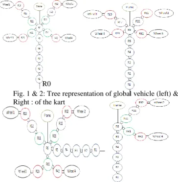
The tree structure is used to draw the reference marks, to raise the arborescence of the mechanism and to define the terminal organs. Figure 1 illustrates the tree structure of global vehicle. The reference R0 is arbitrary defined according to simplified assumptions. The 3D movement of the vehicle is represented by:
𝜉 = [𝑞1, 𝑞2, 𝑞3, 𝑞4, 𝑞5, 𝑞6]𝑇 (1)
These six degrees of freedom are composed by 5 virtual non dynamics bodies and the frame.
- R0 is attached to the ground, R1, R2 … R5 are the virtual bodies which define the posture of the vehicle, and their variables are 𝑞1, 𝑞2, 𝑞3, 𝑞4 𝑎𝑛𝑑 𝑞5;
- R6 is the frame, presented by the variable q6.
The vector of generalized coordinates for the P406, q ∈ R16
is defined as following:
𝑞 = [𝑞𝑖]𝑇with i=1…16, (2)
With R11, R21, R31 and R41 represent the suspension system (𝑞7, 𝑞8, 𝑞9, 𝑞10), R12 and R22 (𝑞11, 𝑞12) the steering locks around the axis z, R13, R32, R23 and R42 (or
𝑞13, 𝑞14, 𝑞15, 𝑞16) are the rotations of four wheels around their
axis y, 𝑞 , 𝑞 ∈ R16
are respectively the vectors of speeds and corresponding generalized accelerations (M’sirdi 2007 [6]).
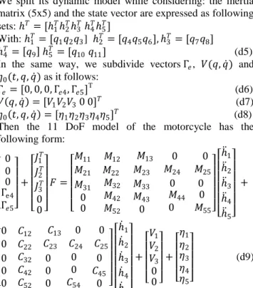
Fig. 1 & 2: Tree representation of global vehicle (left) & Right : of the kart
Fig. 3 left: Tree representation of the quad Fig. 4 right: Tree representation of the motorcycle
Fig. 5: Tree representation of bicycle
We can summarize the DoF belonging to each system in the following table:
R0 P406 QUAD KART MOTO BIKE
DoF 16 15 12 11 9
Table1: DoF for each vehicle C. Dynamic model:
Several formalisms, in the literature, can be used to obtain dynamic models of vehicles. The most often used are: - The formalism of Lagrange (Khalil [7]) (Beurier[8]); - The formalism of Newton-Euler (Khalil [9]).
In this study, we are more interested in the formalism of Lagrange. This formalism describes the equations of the movement in terms of energy which is defined by the following expression:
Γ
𝑖=
𝑑 𝑑𝑡 𝑑𝐿 𝑑𝑞 𝑖−
𝑑𝐿 𝑑𝑞𝑖i=1…n, (3)- With L : Lagrangian of the equal system in E-U ; - E : Total kinetic energy of the system;
- U: Total potential energy of the system.
The vehicle nominal model is developed assuming that the pneumatic contact is permanent and reduced to a single point for each wheel. The dynamics of the vehicle can be described by the passive model (M’sirdi 2004):
𝜏 = 𝑀 𝑞 𝑞 + 𝐶 𝑞, 𝑞 𝑞 + 𝑉 𝑞, 𝑞 + 𝜂0(𝑡, 𝑞, 𝑞 )
𝜏 = Γ𝑒+ Γ = Γ𝑒+ 𝐽𝑇𝐹 𝐹 = 𝑓(𝜆, 𝜎, 𝛼, 𝑞) (4)
The inertia matrix 𝑀(𝑞) of the system is defined in R16x16,
which is a symmetric positive definite matrix. The coefficients of the matrix 𝐶(𝑞, 𝑞 ) of centrifugal and Coriolis forces are established by respecting the property of passivity (M’sirdi [2]).
The vector 𝑉(𝑞, 𝑞 ) is composed by the gravity and frictional forces at the joints.
The vector 𝜂0(𝑡, 𝑞, 𝑞 ) represents the uncertainties and the
neglected dynamics in the vehicle modeling.
The equation (4) demonstrates that input torque consists of two parts; the first part is produced by the active articulations such as motorization, braking and steering. The second one represents the generalized forces due to the contact applied at the terminal organs. These forces of tire-ground contact (longitudinal, lateral and normal of each wheel) are gathered in the vector F.
This Kino-dynamic model, with constraints attached to the tire-ground contact, possesses the following properties:
- P1: The inertia matrix M(q) is Symmetric Positive
Definite (SPD) and its opposite is uniformly restricted.
- P2: With an appropriate definition of 𝐶(𝑞, 𝑞 ) the matrix
𝐴 𝑞, 𝑞 = 𝑀 𝑞 − 2. 𝐶(𝑞, 𝑞 ) is Antisymmetric: 𝑣𝑇𝐴 𝑞, 𝑞 𝑣 = 𝑣𝑇 𝑀 𝑞 − 2. 𝐶 𝑞, 𝑞 𝑣 = 0 ∀𝑣 ∈ 𝑅
- P3: The dynamic equation (4) can be put in a linear
parameter form in a set of dynamic parameter 𝜃 like 𝜏 = 𝜑𝑇𝜃.
The property P1 assures that the effect acceleration function is inertial (stable system). P2 assures that the transfer of 𝜏 − 𝜂0 toward 𝑞 is a passive system and verifies the
inequality of Popov. It assures a sufficient condition of system stability linked to its passivity. These proprieties are verified in the same time as computing the model equation in Maple software.
III. DIVISION OF THE MODEL IN BLOCKS: Our challenge is to describe the vehicle dynamics in terms of blocks and find a common area that connects the five systems studied in paragraph 2. These models have almost the same major components, indeed we have identified five different blocks as follows:
- Translations of the frame (x, y and z); - Rotations of the frame (psi, theta and phi); - Suspension System; - Steering; - Spins wheels.
Afterwards we will split each vehicle in the form of blocks and show that the coupling terms are passive and have low values. Hence the possibility of applying our observers and robust command, and switch easily between different systems.
We subdivided the vehicles into three subsets as follows: - The global model is P406 which is the biggest model; - Second subset contains Quad and motorcycle; - Third subset includes kart and bike.
A. First application for a car (P406): We split the car dynamic model while considering: the inertia matrix (5x5) and the state vector are expressed as following sets (M’sirdi IROS [10]): ℎ𝑇= [ℎ
1 𝑇ℎ 2 𝑇ℎ 3 𝑇ℎ 4 𝑇ℎ 5 𝑇] With:ℎ1𝑇 = [𝑞1𝑞2𝑞3]ℎ𝑇2 = [𝑞4𝑞5𝑞6], ℎ3𝑇 = [𝑞7𝑞8𝑞9𝑞10], ℎ3𝑇= [𝑞11𝑞12]ℎ4𝑇 = [𝑞13𝑞14𝑞15𝑞16] (a5)
In the same way, we subdivide vectors Γ𝑒, 𝑉(𝑞, 𝑞 ) and
𝜂0(𝑡, 𝑞, 𝑞 ) as it follows:
Γ𝑒 = [0, 0, 0, Γ𝑒3, Γ𝑒4]T (a6)
𝑉 𝑞, 𝑞 = [𝑉1𝑉2 𝑉3 0 0]𝑇 (a7)
𝜂0 𝑡, 𝑞, 𝑞 = [𝜂1𝜂2𝜂3𝜂4𝜂5]𝑇 (a8)
The 16 DoF model of the car has the following form:
0 0 0 Γe4 Γ𝑒5 + 𝐽1𝑇 𝐽2𝑇 𝐽3𝑇 0 0 𝐹 = 𝑀11 𝑀12 𝑀13 0 0 𝑀21 𝑀22 𝑀23 𝑀24 𝑀25 𝑀31 0 0 𝑀32 𝑀42 𝑀52 𝑀33 𝑀43 0 0 0 𝑀44 0 0 𝑀55 ℎ1 ℎ 2 ℎ 3 ℎ 4 ℎ 5 + 0 𝐶12 𝐶13 0 0 0 𝐶22 𝐶23 𝐶24 𝐶25 0 0 0 𝐶32 𝐶42 𝐶52 0 0 0 00 𝐶54 0 𝐶45 0 ℎ1 ℎ 2 ℎ 3 ℎ 4 ℎ 5 + 𝑉1 𝑉2 𝑉3 0 0 + 𝜂1 𝜂2 𝜂3 𝜂4 𝜂5 (a9)
The model is described by five equations which correspond respectively to the frame translations, frame rotations, suspension system, the steering and the wheels rotations. From this new representation, we obtain the forces translations as following: (a10)
𝐹𝑇= 𝐽1𝑇𝐹 = 𝑀11ℎ 1+ 𝑀12ℎ 2+ 𝑀13ℎ 3+ 𝐶12ℎ 2+ 𝐶13ℎ 3+ 𝑉1+ 𝜂1 The next equation describes the frame rotations forces.
𝐹𝑅= 𝐽2𝑇𝐹 = 𝑀21ℎ 1+ 𝑀22ℎ 2+ 𝑀23ℎ 3+ 𝑀24ℎ 4+
𝑀25ℎ 5+ 𝐶22ℎ 2+ 𝐶23ℎ 3+ 𝐶24ℎ 4+ 𝐶25ℎ 5+ 𝑉2+ 𝜂2 (a11)
The equation below represents the forces of suspension system (four dampers): (a12)
𝐹𝑠𝑢𝑠𝑝 = 𝐽3𝑇𝐹 = 𝑀31ℎ 1+ 𝑀32ℎ 2+ 𝑀33ℎ 3+ 𝐶32ℎ 2+ 𝑉3+ 𝜂3
The forces of steering and wheels rotations are: (a13)
Г𝑒4= 𝑀42ℎ 2+ 𝑀43ℎ 3+ 𝑀44 ℎ 4+ 𝐶42ℎ 2+ 𝐶45ℎ 5+ 𝑉4+ 𝜂4
Г𝑒5= 𝑀52ℎ 2+ 𝑀55ℎ 5+ 𝐶52ℎ 2+ 𝐶54ℎ 4+ 𝑉5+ 𝜂5 (a14)
Most of the researchers neglect the effect of coupling terms. The spitting of the 16 DoF model is rich in terms of data, especially, the evolution of the coupling terms 𝜂𝑐𝑖 which
connect the different submodels. We can show that these variables are bounded ∀t and the submodels can be written: 11 : ℎ 1= 𝑓1 ℎ1, ℎ 1, 𝐹𝑇 + 𝜂𝑐1 (a15)
12 : ℎ 2= 𝑓2 ℎ2, ℎ 2, 𝐹𝑅 + 𝜂𝑐2 (a16)
2 : ℎ 3= 𝑓3 ℎ3, ℎ 3, 𝐹𝑠𝑢𝑠𝑝 + 𝜂𝑐3 (a17)
31 : ℎ 4= 𝑓4 ℎ4, ℎ 4, Г𝑒4 + 𝜂𝑐4 (a18)
32 : ℎ 5= 𝑓5 ℎ5, ℎ 5, Г𝑒5 + 𝜂𝑐5 (a19)
A.1. Representation in 3 subsystems: - Movements of the frame: The equation (a20) gives a general frame representation (translation and rotation):
1 𝐹𝑇 𝐹𝑅 = 𝑀11 𝑀12 𝑀21 𝑀22 ℎ 1 ℎ 2 + 𝐶12 𝐶22 ℎ 2+ 𝑉1 𝑉2 + 𝜂𝑐1 𝜂𝑐2 (a20)
The two coupling terms 𝜂𝑐1 and 𝜂𝑐2 verify:
𝜂𝑐1= 𝑀13ℎ 3+ 𝐶13ℎ 3+ 𝜂1 (a21)
𝜂𝑐2= 𝑀23ℎ 3+ 𝑀24ℎ 4+ 𝑀25ℎ 5+ 𝐶23ℎ 3+ 𝐶24ℎ 4+
𝐶25ℎ 5+ 𝜂2 (a22)
By choosing the state variables 𝑥11= (ℎ1, ℎ2) and 𝑥12=
(ℎ 1, ℎ 2). We have the following state representation:
𝑥 11 = 𝑥12 𝑥 12= 𝑀1−1(𝐽12𝑇𝐹 − 𝐶1𝑥12− 𝑉12− 𝜇1) 𝑦1 = 𝑠 𝑥11, 𝑥12 (a23) With:𝑀1= 𝑀𝑀11 𝑀12 21 𝑀22 , 𝐶1= 𝐶12 𝐶22 , 𝐽12 𝑇 = 𝐽1𝑇 𝐽2𝑇 ,𝑉12= 𝑉1 𝑉2 and 𝜇1= 𝜂𝑐 1
𝜂𝑐2 Which are respectively the inertia matrix,
the matrix of centrifugal and Coriolis forces, the reduced Jacobian matrix, vector gravity and the vector of coupling terms linked to the first sub system.
- Suspension system:
The suspension system ( 2) contains the fours suspensions in the car.
𝐹𝑠𝑢𝑠𝑝 = 𝑀33ℎ 3+ 𝑉3+𝜂𝑐3 (a24)
𝜂𝑐3= 𝑀31ℎ 1+ 𝐶32ℎ 2+ 𝑀32ℎ 2+ 𝜂3.
Let𝑥2= ( 𝑥21, 𝑥22) = (ℎ3, ℎ 3), the state space
representation of the subsystem ( 2) is then: 𝑥 21= 𝑥22 𝑥 22= 𝑀1−1(𝐽3𝑇𝐹 − 𝑉3− 𝜇2) 𝑦2= 𝑠 𝑥21, 𝑥22 (a25) Where 𝜇2= 𝜂𝑐3 - Dynamic of wheels:
The wheels dynamic ( 3) contains two blocks: the steering of the two front wheels ( 31) and the rotations of four wheels following their axis y( 32).
The equations (a13, a14) give the following dynamic model: Г𝑒4 = 𝑀44ℎ 4+ 𝐶45ℎ 5+ 𝜂𝑐4 (a26)
Г𝑒5= 𝑀55ℎ 5+ 𝐶54ℎ 4+ 𝜂𝑐5 (a27)
By identification, we obtain the coupling terms 𝜂𝑐4 and 𝜂𝑐5 :
𝜂𝑐4= 𝑀42ℎ 2+ 𝑀43ℎ 3+ 𝐶42ℎ 2+ 𝜂4 (a28)
𝜂𝑐5= 𝑀52ℎ 2+ 𝐶52ℎ 2+ 𝜂5 (a29)
If we combine the equations together we will have: Γ𝑒4 Γ𝑒5 = 𝑀44 0 0 𝑀55 ℎ 4 ℎ 5 + 0 𝐶𝐶 34 43 0 ℎ 4 ℎ 5 + 𝜂𝑐4 𝜂𝑐5 (a30)
For the same reasoning, we chose the state variables 𝑥21 = (ℎ4, ℎ5) and 𝑥22= (ℎ 4, ℎ 5), in order to obtain the
following state representation : 𝑥 21= 𝑥22 𝑥 22= 𝑀2−1 Γ𝑒45− 𝐶2𝑥22− 𝜇3 𝑦2= 𝑠 𝑥21, 𝑥22 (a31) With : 𝑀2= 𝑀044 𝑀0 55 ,𝐶2= 0 𝐶45 𝐶54 0 ,Γ𝑒45 = Γ𝑒4 Γ𝑒5 , and 𝜇3= 𝜂𝑐 4
𝜂𝑐5 Which are respectively the reduced inertia
matrix, the reduced matrix of centrifugal and Coriolis forces, the vector of input torque and the vector of coupling terms attached to the third sub system.
B. Second application for a Quad:
Quad is an all-terrain vehicle, also known as a four-wheeler, with one seat that is straddled by the driver, along with handlebars for steering control.
It has only three dampers-springs: - Two front dampers-springs; - Single rear damper-spring.
We split the dynamic model while considering: the inertia matrix (5x5) and the state vector are expressed as following sets: ℎ𝑇 = [ℎ 1 𝑇ℎ 2 𝑇ℎ 3 𝑇ℎ 4 𝑇ℎ 5 𝑇] With:ℎ1𝑇 = [𝑞1𝑞2𝑞3]ℎ2𝑇 = [𝑞4𝑞5𝑞6], ℎ3𝑇 = [𝑞7𝑞8 𝑞9], ℎ3𝑇 = [𝑞10𝑞11]ℎ4𝑇 = [𝑞12𝑞13𝑞14𝑞15] (b5)
In the same way, we subdivide vectors Γ𝑒, 𝑉(𝑞, 𝑞 ) and
𝜂0(𝑡, 𝑞, 𝑞 ) as it follows:
Γ𝑒 = [0, 0, 0, Γ𝑒3, Γ𝑒4]T (b6)
𝑉 𝑞, 𝑞 = [𝑉1𝑉2 𝑉3 0 0]𝑇 (b7)
𝜂0 𝑡, 𝑞, 𝑞 = [𝜂1𝜂2𝜂3𝜂4𝜂5]𝑇 (b8)
0 0 0 Γe4 Γ𝑒5 + 𝐽1𝑇 𝐽2𝑇 𝐽3𝑇 0 𝐽5𝑇 𝐹 = 𝑀11 𝑀12 𝑀13 0 0 𝑀21 𝑀22 𝑀23 𝑀24 𝑀25 𝑀31 0 0 𝑀32 𝑀42 𝑀52 𝑀33 𝑀43 0 0 0 𝑀44 0 0 𝑀55 ℎ1 ℎ 2 ℎ 3 ℎ 4 ℎ 5 + 0 𝐶12 𝐶13 0 0 0 𝐶22 𝐶23 𝐶24 𝐶25 0 0 0 𝐶32 𝐶42 𝐶52 0 0 0 0 0 𝐶54 0 𝐶45 0 ℎ1 ℎ 2 ℎ 3 ℎ 4 ℎ 5 + 𝑉1 𝑉2 𝑉3 0 0 + 𝜂1 𝜂2 𝜂3 𝜂4 𝜂5 (b9)
The model is described by five equations which correspond respectively to the frame translations, frame rotations, suspension system, the steering and the wheels rotations. In conclusion, the difference with the previous car model is in the equation (b9) at the Jacobian level. The term 𝐽5𝑇 is for
description of the single back suspension axle-tree. Thus it will change the block of wheels rotations.
C. Third application for a kart:
The Kart which we dispose is a kind of battery-driven vehicle equipped with 4 mass OPTIMA batteries and an engine with separate excitement (brushless). The maximum speed is about 70 Km/h [H. NASSER, N.K. [11]]. It is generally accepted as the most economic form of motorsport available. Also wheels and tires are much smaller than those used on a normal car. Missing of a suspension system reduces the model of 4 DoF compared to the 16 DoF model of Peugeot 406 (M’sirdi 2004, 2007). We split the previous dynamic model while considering: the inertia matrix (5x5) and the state vector is expressed as following sets: ℎ𝑇= [ℎ 1 𝑇ℎ 2 𝑇0 ℎ 3 𝑇ℎ 4 𝑇] With: ℎ1𝑇 = [𝑞1𝑞2𝑞3] ℎ2𝑇 = [𝑞4𝑞5𝑞6], ℎ3𝑇= [𝑞7𝑞8] ℎ4𝑇 = [𝑞9𝑞10𝑞11𝑞12] (c5)
In the same way, we subdivide vectors Γ𝑒, 𝑉(𝑞, 𝑞 ) and
𝜂0(𝑡, 𝑞, 𝑞 ) as it follows:
Γ𝑒 = [0, 0, 0, Γ𝑒4, Γ𝑒5]T (c6)
𝑉 𝑞, 𝑞 = [𝑉1𝑉20 0 0]𝑇 (c7)
𝜂0 𝑡, 𝑞, 𝑞 = [𝜂1𝜂20 𝜂4𝜂5]𝑇 (c8)
The 12 Dof model of the kart has the following form: 0 0 0 Γe4 Γ𝑒5 + 𝐽1𝑇 𝐽2𝑇 0 0 0 = 𝑀11 𝑀12 0 0 0 𝑀21 𝑀22 0 𝑀23 𝑀24 0 0 0 0 0 𝑀32 0 𝑀42 0 0 𝑀33 0 0 0 𝑀44 ℎ1 ℎ 2 0 ℎ 3 ℎ 4 + 0 𝐶12 0 0 0 0 𝐶22 0 𝐶23 𝐶24 0 0 0 0 0 𝐶32 0 𝐶42 0 0 0 𝐶43 0 𝐶34 0 ℎ1 ℎ 2 0 ℎ 3 ℎ 4 + 𝑉1 𝑉2 0 0 0 + 𝜂1 𝜂2 0 𝜂4 𝜂5 (c9)
The model is described by four equations which correspond respectively to the frame translations, frame rotations, the steering and the wheels rotations.
From this new representation, we estimate the forces translations as following:
𝐹𝑇= 𝐽1𝑇𝐹 = 𝑀11ℎ 1+ 𝑀12ℎ 2+ 𝐶12ℎ 2+ 𝑉1+ 𝜂1 (c10)
The next equation describes the forces rotations of the frame.
𝐹𝑅= 𝐽2𝑇𝐹 = 𝑀21ℎ 1+ 𝑀22ℎ 2+ 𝐶22ℎ 2+ 𝐶23ℎ 3+ 𝐶24ℎ 4+
𝑉2+ 𝜂2 (c11)
The forces of steering and wheels rotations are:
Г𝑒4= 𝑀32ℎ 2+ 𝑀33ℎ 3+ 𝐶32ℎ 2+ 𝐶34ℎ 4+ 𝑉3+ 𝜂4 (c12)
Г𝑒5= 𝑀42ℎ 2+ 𝑀44ℎ 4+ 𝐶42ℎ 2+ 𝐶43ℎ 3+ 𝑉4+ 𝜂5 (c13)
The spitting of the 12 DoF model can be written as: 11 : ℎ 1= 𝑓1 ℎ1, ℎ 1, 𝐹𝑇 + 𝜂𝑐1 (c14)
12 : ℎ 2= 𝑓2 ℎ2, ℎ 2, 𝐹𝑅 + 𝜂𝑐2 (c15)
31 : ℎ 3= 𝑓3 ℎ3, ℎ 3, Г𝑒3 + 𝜂𝑐4 (c16)
32 : ℎ 4= 𝑓4 ℎ4, ℎ 4, Г𝑒4 + 𝜂𝑐5 (c17)
C.1 Representation in 2 under systems:
Movements of the frame: The equation (c18) gives a general frame representation (translation and rotation): 1:
𝐹𝑇 𝐹𝑅 = 𝑀11 𝑀12 𝑀21 𝑀22 ℎ 1 ℎ 2 + 𝐶12 𝐶22 ℎ 2+ 𝑉1 𝑉2 + 𝜂𝑐1 𝜂𝑐2 (c18)
The two coupling terms 𝜂𝑐1 and 𝜂𝑐2 verify:
𝜂𝑐1= 𝜂1 (c19)
𝜂𝑐2= 𝑀23ℎ 3+ 𝑀24ℎ 4+ 𝐶23ℎ 3+ 𝐶24ℎ 4+ 𝜂2 (c20)
By choosing the state variables 𝑥11= (ℎ1, ℎ2) and 𝑥12= (ℎ 1, ℎ 2). We have the following state representation:
𝑥 11 = 𝑥12 𝑥 12= 𝑀1−1(𝐽12𝑇𝐹 − 𝐶1𝑥12− 𝑉12− 𝜇1) 𝑦1= 𝑠 𝑥11, 𝑥12 (c21) With:𝑀1= 𝑀𝑀11 𝑀12 21 𝑀22 , 𝐶1= 𝐶12 𝐶22 , 𝐽12 𝑇 = 𝐽1𝑇 𝐽2𝑇 , 𝑉12= 𝑉1 𝑉2 and 𝜇1= 𝜂𝑐1
𝜂𝑐2 Which are respectively the inertia
matrix, the matrix of centrifugal and Coriolis forces, the reduced Jacobian matrix, vector gravity and the vector of coupling terms linked to the first sub system.
Dynamic of wheels:
The wheels dynamic ( 2) contains two blocks: the steering of the two front wheels ( 31) and the rotations of four wheels following their axis y( 32).
The eq(c12, c13) give the following dynamic model: Г𝑒3= 𝑀33ℎ 3+ 𝐶34ℎ 4+ 𝜂𝑐4 (c22)
Г𝑒4= 𝑀44ℎ 4+ 𝐶43ℎ 3+ 𝜂𝑐5 (c23)
By identification, we obtain the coupling terms 𝜂𝑐4 and 𝜂𝑐5 :
𝜂𝑐4= 𝑀32ℎ 2+ 𝐶32ℎ 2+ 𝜂4 (c24)
𝜂𝑐5= 𝑀42ℎ 2+ 𝐶42ℎ 2+ 𝜂5 (c25)
If we combine the equations together we will have: Γ𝑒4 Γ𝑒5 = 𝑀33 0 0 𝑀44 𝑞 3 𝑞 4 + 0 𝐶34 𝐶43 0 𝑞 3 𝑞 4 + 𝜂𝑐4 𝜂𝑐5 (c26)
For the same reasoning, we chose the state variables 𝑥21 = (ℎ3, ℎ4) and 𝑥22= (ℎ 3, ℎ 4), in order to obtain the
following state representation : 𝑥 21= 𝑥22 𝑥 22= 𝑀2−1 Γ𝑒45− 𝐶2𝑥22− 𝜇2 𝑦2= 𝑠 𝑥21, 𝑥22 (c27) With : 𝑀2= 𝑀033 𝑀0 44 ,𝐶2= 0 𝐶34 𝐶43 0 ,Γ𝑒45 = Γ𝑒4 Γ𝑒5 , and 𝜇3= 𝜂𝑐 4
𝜂𝑐5 Which are respectively the reduced inertia
matrix, the reduced matrix of centrifugal and Coriolis forces, the vector of input torque and the vector of coupling terms attached to the second sub system. In conclusion the main difference with previous models is that there is no suspension dynamics (one line and one column disappear from inertial matrix and Coriolis and centrifuge matrix. The coupling terms are simpler as consequence.
A motorcycle is a single-track, two-wheeled motor vehicle. Different types of motorcycles have different dynamics and these play a role in how a motorcycle performs in given conditions.
We split its dynamic model while considering: the inertia matrix (5x5) and the state vector are expressed as following sets: ℎ𝑇= [ℎ 1 𝑇ℎ 2 𝑇ℎ 3 𝑇 ℎ 4𝑇ℎ5𝑇] With: ℎ1𝑇 = [𝑞1𝑞2𝑞3] ℎ2𝑇 = [𝑞4𝑞5𝑞6], ℎ3𝑇= [𝑞7𝑞8] ℎ4𝑇 = 𝑞9 ℎ5𝑇= [𝑞10 𝑞11] (d5)
In the same way, we subdivide vectors Γ𝑒, 𝑉(𝑞, 𝑞 ) and
𝜂0(𝑡, 𝑞, 𝑞 ) as it follows:
Γ𝑒 = [0, 0, 0, Γ𝑒4, Γ𝑒5]T (d6)
𝑉 𝑞, 𝑞 = [𝑉1𝑉2𝑉3 0 0]𝑇 (d7)
𝜂0 𝑡, 𝑞, 𝑞 = [𝜂1𝜂2𝜂3𝜂4𝜂5]𝑇 (d8)
Then the 11 DoF model of the motorcycle has the following form: 0 0 0 Γe4 Γ𝑒5 + 𝐽1𝑇 𝐽2𝑇 𝐽3𝑇 0 0 𝐹 = 𝑀11 𝑀12 𝑀13 0 0 𝑀21 𝑀22 𝑀23 𝑀24 𝑀25 𝑀31 0 0 𝑀32 𝑀42 𝑀52 𝑀33 𝑀43 0 0 0 𝑀44 0 0 𝑀55 ℎ1 ℎ 2 ℎ 3 ℎ 4 ℎ 5 + 0 𝐶12 𝐶13 0 0 0 𝐶22 𝐶23 𝐶24 𝐶25 0 0 0 𝐶32 𝐶42 𝐶52 0 0 0 0 0 𝐶54 0 𝐶45 0 ℎ1 ℎ 2 ℎ 3 ℎ 4 ℎ 5 + 𝑉1 𝑉2 𝑉3 0 0 + 𝜂1 𝜂2 𝜂3 𝜂4 𝜂5 (d9)
The model is described by five equations which correspond respectively to the frame translations, frame rotations, suspension system, the steering and the wheels rotations. Basing on equation (d9), we constate that the form is similar to the P406 model.
E. Fifth application for a bicycle:
Bicycle, also known as bike, is a pedal-driven, having two wheels attached to frame which one behind the other. We considered a bike without any suspension system and we subdivide bicycle dynamic model while considering: the inertia matrix and the state vector are expressed as following: ℎ𝑇 = [ℎ 1 𝑇ℎ 2 𝑇0 ℎ 3𝑇ℎ4𝑇] With: ℎ1𝑇 = [𝑞1𝑞2𝑞3] ℎ2𝑇 = [𝑞4𝑞5𝑞6], ℎ3𝑇= [𝑞7] ℎ4𝑇 = [𝑞8𝑞9] (e5)
In the same way, we subdivide vectors Γ𝑒, 𝑉(𝑞, 𝑞 ) and
𝜂0(𝑡, 𝑞, 𝑞 ) as it follows:
Γ𝑒 = [0, 0, 0, Γ𝑒3, Γ𝑒4]T (e6)
𝑉 𝑞, 𝑞 = [𝑉1𝑉20 0 0]𝑇 (e7)
𝜂0 𝑡, 𝑞, 𝑞 = [𝜂1𝜂20 𝜂3𝜂4]𝑇 (e8)
The model is described by four equations which correspond respectively to the frame translations, frame rotations, the steering and the wheels rotations.
Then the 9dof model of the bicycle has the following form: 0 0 0 Γe3 Γ𝑒4 + 𝐽1𝑇 𝐽2𝑇 0 0 0 = 𝑀11 𝑀12 0 0 0 𝑀21 𝑀22 0 𝑀23 𝑀24 0 0 0 0 0 𝑀32 0 𝑀42 0 0 𝑀33 0 0 0 𝑀44 ℎ1 ℎ 2 0 ℎ 3 ℎ 4 + 0 𝐶12 0 0 0 0 𝐶22 0 𝐶23 𝐶24 0 0 0 0 0 𝐶32 0 𝐶42 0 0 0 𝐶43 0 𝐶34 0 ℎ1 ℎ 2 0 ℎ 3 ℎ 4 + 𝑉1 𝑉2 0 0 0 + 𝜂1 𝜂2 0 𝜂3 𝜂4 (e9)
In this case, we note that forces and coupling terms have similar form as the electrical kart (see P3.3).
F. Interpretation:
To summarize, the following figure 6 describes the five blocks of the global and the second subset (the frame translations, frame rotations, suspension system, the steering and the wheels rotations).
Fig.6: the 5 blocks of the P406, Quad and motorcycle The following figure 7 describes the four blocks of the third subset (the frame translations, frame rotations, the steering and the wheels rotations) with no suspension system. The 4 blocks of kart and bike dynamic models acquire the same properties as the global system (see paragraph 2). Thus it is important to remark that the coupling terms and the uncertainties of modeling, estimation and noises are going to appear in the same way as passive inputs in the system. So they will be dissipated.
It will be the same for other sub systems of the nominal model, because the same reasoning applies “mutatis mutandis”. The importance of our approach shows that the employement of the neglected terms are well chosen. In this paper we consider the car as a parent agent and quad, kart, motorcycle and bicycle as its descendants. In fact, the reference dynamic model is the 16 DoF model which we will identify blocks of each descendant in this global model to facilitate any task switching from one system to another or from one structure to another. The table 2 shows a correlation between the kart and a P406 models as follows:
- The dashed blocks represent the dynamics of the kart; - The not dashed blocks represent the dynamics provided by the four suspensions of P406.
With this strategy we can classify the five models using only the global car model for ambitions goals such as drawing, motion analysis and diagnosis…
IV. SIMULATION
V.
The dynamic model of the kart without contact is generated with the symbolic calculations software (Maple).
0 100 200 300 400 500 600 700 800 900 1000 -4000 -3000 -2000 -1000 0 1000 2000 3000 4000 Time ms J TF r1 N nuc21 Torque1 0 500 1000 1500 2000 2500 3000 3500 4000 4500 5000 -1000 -500 0 500 1000 1500 time (ms) t o r q u e torque 0 500 1000 1500 2000 2500 3000 3500 4000 4500 5000 -80 -60 -40 -20 0 20 40 time(ms) c o u p li n g t e r m nuc4 0 500 1000 1500 2000 2500 3000 3500 4000 4500 5000 -1 -0.8 -0.6 -0.4 -0.2 0 0.2 0.4 0.6 0.8 1x 10 4 t o r q u e compared torque 0 500 1000 1500 2000 2500 3000 3500 4000 4500 -200 -150 -100 -50 0 50 100 150 200 Time (ms) c o u p li g t e rm nuc5 To validate this decoupled model, detailed in the previous paragraph, we used a modified simulator version of (SimK106N) (G. Beurier [8] M’sirdi [12]). For this simulation, we apply a constant direction -0.7°;
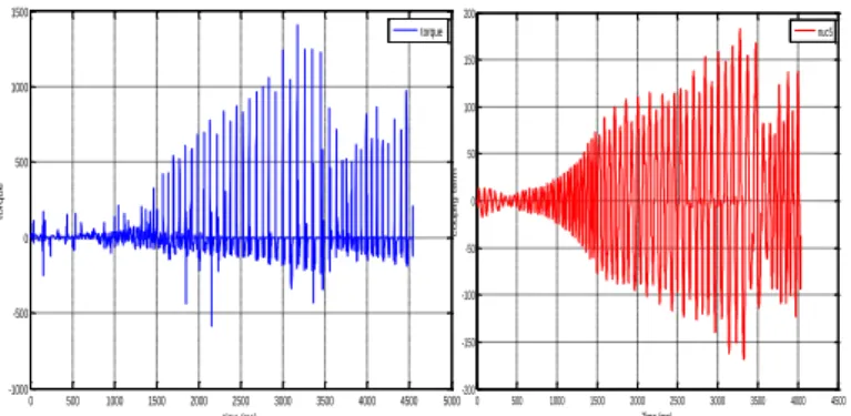
So we will take the kart model for the following simulation as an example to analyze the evolution of coupling terms compared with torques.
Figure 9:The evolution of 2nd coupling term
We compared the terms of the equations c21. We observe that the amplitudes of coupling terms are lower than the input torque (fig. 9). The absence of a suspension system on the kart is translated by vibration of these parameters. On a normal car the coupling terms 𝜂𝑐𝑖 are passive and converge to zero.
Figure 10.a: The evolution of compared torque Figure 10.b: The evolution of 4rd coupling term
Even, we can neglect the 4rdcoupling term to the compared torques (see Fig. 10 and equation c27). On the other side, the excellent attenuation of 𝜂𝑐𝑖 in the case of a car is
explained by the absorption of these parameters at the suspension system level.
Figure 11.a: The evolution of steering torque term Figure 11.b: The evolution of 5th coupling term
Using equation c27, we obtain figure 11 which shows that the 5th coupling term is smaller than the amplitudes of the torque of wheels rotations and it can be neglected. Also the equation (c19) proves that the 1stcoupling term is equal to a neglected term 𝜂1because of the absence of a suspension system.
VI. CONCLUSION
In this paper, a 16 DoF global dynamic model of a car is developed and exploited with its suspension system. This geometrical and kinematics model takes into account the unknown tire–ground contact forces. For diagnosis purpose based on decentralized robust observers, we split the model in sub-blocks in order to illustrate the passivity of the global system and the sub systems. We have also compared dynamics of 5 vehicles. This comparison allows understanding the rationale of the behavior of vehicles in perspectives this will be used for control design and diagnosis. The simulator (SimK106N) was transformed to simulate the dynamic model of five kind of vehicles, allowed us to appreciate the coupling energy level flowing through the whole systems.
REFERENCES
[1] N.K. M'sirdi, A. Rabhi, N. Zbiri, and Y. Delanne: VRIM: Vehicle
Road Interaction Modelling for Estimation of Contact Forces. Accepted
for TMVDA 04. 3rd Int. Tyre Colloquium Tyre Models For Vehicle Dynamics Analysis August 30-31, 2004 University of Technology Vienna. [2] N.K. M'Sirdi, A. Rabhi, Aziz Naamane: Vehicle models and
estimation of contact forces and tire road friction". Invited paper ICINCO:
351-358, 2007.
[3] H.B. Pacejka.: Simplified behavior of steady state turning behavior of
motor vehicles, part 1: Handling diagrams and simple systems. Vehicle System Dynamics 2 1973, pp. 162 - 172.
[4] B. Jaballah- NK M'sirdi - A Naamane, M. Hassani "Estimation of
Longitudinal and Lateral Velocity of Vehicle" , "17th IEEE Mediterranean
Conference on Control and Automation (MED'09).
[5] A Rabhi, NK M'sirdi A Naamane, B Jaballah. Vehicle Velocity Estimation Using Sliding Mode Observers" , in : IEEE, "9th int conf
Sciences and Techniques of Automatic, STA'2008
[6] K. N. M'sirdi, L. H. Rajaoarisoa, J.-F. Balmat, J. Duplaix: Modeling
for Control and diagnosis for a class of Non Linear complex switched systems. Advances in Vehicle Control and Safety AVCS 07, Buenos Aires,
Argentine, February 8-10, 2007.
[7] Khalil w. “Dynamic modelling and identification of a car” 2002 CIFA. [8] G. Beurier Thèse de doctorat de l’UPMC, Paris 6.
[9] Khalil w. Kleinfinger J-F “minimum operations and minimum
parameters of the dynamic model of tree structure robots” IEEE of
Robotics and Automation, déc. 1987
[10] N.K. M'sirdi, B. Jaballah, A. Naamane, H. Messaoud: Robust
Observers and Unknown Input Observers for estimation, diagnosis and control of vehicle dynamics, IEEE/RSJ International Conference on IROS.
[11] H Nasser, N.K. M'Sirdi, , A Naamane « Inboard observers and
sensors for an electrical and autonomous kart” STA 2008.
[12] N. K. M'Sirdi. « Observateurs robustes et estimateurs pour
l'estimation de la dynamique des véhicules et du contact pneu – route ».