Nanoparticles and Taylor Dispersion as a Linear Time-Invariant
System
Philipp Lemal,
†Alke Petri-Fink,
†,‡and Sandor Balog
*
,††Adolphe Merkle Institute, University of Fribourg, Chemin des Verdiers 4, 1700 Fribourg, Switzerland ‡Chemistry Department, University of Fribourg, Chemin du Musée 9, 1700 Fribourg, Switzerland
*
S Supporting InformationABSTRACT: The physical principles underpinning Taylor dispersion offer a high dynamic range to characterize the hydrodynamic radius of particles. While Taylor dispersion grants the ability to measure radius within nearly 5 orders of magnitude, the detection of particles is never instantaneous. It requires afinite sample volume, a finite detector area, and a finite detection time for measuring absorbance. First we show that these practical requirements bias the analysis when the self-diffusion coefficient of particles is high, which is typically the case of small nanoparticles. Second we show that the accuracy of the technique may be recovered by treating Taylor dispersion as a linear time-invariant system, which we prove by analyzing the Taylor dispersion spectra of two iron-oxide nanoparticles measured under
identical experimental conditions. The consequence is that such treatment may be necessary whenever Taylor dispersion analysis is not optimized for a given size but dedicated to characterize broad groups of particles of varying size and material.
C
haracterizing the size of particles dispersed or suspended in viscoelastic media is fundamental in many fields of academic research and also has strong implication for industrial manufacturing processes. Indeed, size defines several phys-icochemical properties, including but not limited to catalytic reactivity, dissolution rate, appearance, and stability in, e.g., inks and paints, delivery of drug formulations, and texture and mouthfeel in food science.The traditional experimental techniques dedicated to particle size analysis are transmission and scanning electron microscopy, dynamic light scattering, particle tracking analysis, small-angle X-ray, and neutron scattering. Thefirst attempt of adopting Taylor dispersion1−3 to characterize colloidal particles was successful,4 yet the technique was not attracting immediate attention from the communities interested in particles. Fortunately, the technique now appears to be experiencing a renaissance, and thus, currently there is an active interest in implementing the technique for particle systems, including organic, inorganic, metallic, and nonmetallic particles.5−12
Taylor dispersion is the combination of three independent phenomena: optical extinction, translational self-diffusion, and sheer-enhanced dispersion of particles subjected to a steady laminar flow in a microfluidic channel, usually driven by a pressure gradient in a cylindrical capillary tube. The velocity profile of the laminar flow disperses the homogeneous band of the injected particles, which creates a concentration and induces a spontaneous net transport of particles via transla-tional self-diffusion. As a result, the band broadens.7 The rate of band-broadening is defined by the velocity profile and translational diffusion coefficient of the particles. The
hydro-dynamic radius is determined from the self-diffusion coefficient (D) via the Stokes−Einstein equation (D = kBT/6πηr),13−15
and D is determined through analyzing the so-called “taylorgram”, which is the temporal record of the optical absorbance of the particle band at a given distance from the injection point. Given the Lambert−Beer law and a linear detector response, the taylorgram of uniform particles of hydrodynamic radius r resulting from an ideal experiment, where the injected sample band and detection volumes are infinitely thin, is written as1−3
= − − δ
A r t t( , ; )0 a t t0/ e (t t0) /rt 2
(1) where a is the amplitude,δ = πηY2k T2
B , Y the capillary radius,η the
viscosity of the fluid, T the temperature, kB the Boltzmann
constant, and t0= x/v, the so-called residence time defined by
the distance between detection and injection points (x = xdet−
xinj) and the mean velocity of theflow (v) averaged over the
cross section of the capillary.Equation 1is essentially a time-dependent Gaussian function, whose width increases with the residence time and particle size. Therefore, by determining the residence time and the width of the absorbance profile, one can determine the hydrodynamic radius. Classical Taylor dis-persion requires that (i) the Reynolds number (2ρYv/η, where ρ is the density of the fluid) is small, (ii) the rate of axial diffusion of the particles in the tubes is small compared to convection, that is, the inequality 69≤ vY/D (Peclet number)
http://doc.rero.ch
Published in "Analytical Chemistry 91(2): 1217–1221, 2019"
which should be cited to refer to this work.
is satisfied, and (iii) the residence time is much larger than the characteristic (dimensionless) diffusion time on a distance equal to the capillary radius, that is, the inequality 1.4≤ tD=
Dt0/Y2 is satisfied. Cottet et al. showed that these conditions
could be considerably eased if the user tolerates the consequent small relative error.16
It has been recognized early that even if the vital experimental conditions are fulfilled, the profile given by eq 1, where the sample and detection volumes are described by Dirac delta functions, is in fact never truly attained in real experiments. The exact theoretical profile may be closely approximated by a careful instrument design where systematic errors may be treated as very small perturbations. In these cases, corrections may be applied to adjust the experimentally derived values, such as residence time and profile variance.17If the range of diffusion coefficients is known a priori, to optimize the experiment is straightforward. In other words, for a given range of particle sizes, one may alwaysfind a valid combination of operation parameters that ensures that the analysis is of high quality.16,18
While careful instrument design is the essence of any analytical technique, the practice of Taylor dispersion aims to achieve a status similar to that of dynamic light scattering, in a sense that one single instrument and the related analysis should be able to address a wide range of particle sizes without the need of calibrating and validating new operation parameters from one particle system to another, which is not only sluggish but promotes fragile traceability. Indeed, the capillary diameter, the distance, and the size of the capillary window are not varied routinely but changed only when the capillary is replaced. Routinely adjustable parameters are driving pressure, ramp time, and injected sample volume. This is crucial when considering that weakly absorbing (or scattering7) suspensions require relatively large sample and detection volume that cannot be treated as small errors.17
In order to unfold the high dynamic range, inherent in Taylor dispersion, with one single instrument and afixed set of operational parameters, we reconstructeq 1for arbitrary large perturbations. Our basis is given by recognizing that Taylor dispersion may be treated as a linear time-invariant system, where the impulse response function has essential importance in the description of the system (Figure 1).
Since Taylor dispersion is a linear time-invariant system,eq 1 describes exactly the impulse-response function of an ideal Taylor dispersion setup.19 The behavior of a linear time-invariant system is described completely by its impulse
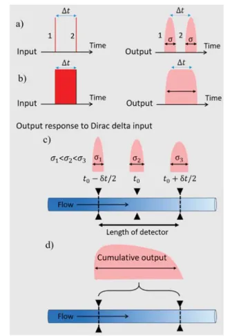
response, and hence the output to any arbitrary input can be calculated. The linearity is ensured by the characteristics of the differential equation governing the dynamics of the particle concentration.1,20 Linear systems have the property that the input is linearly related to the output. Changing the input in a linear way will change the output in the same linear way. Accordingly, linear combinations of distinct inputs will produce linear combinations of the related outputs. Time-invariant systems have the property that the form of the output for a given input does not depend on when that input was applied (Figure 2a,b). Furthermore, Taylor dispersion is integrative in the output (Figure 2c,d).
This is the approach we will adopt in this letter to describe
eq 1in experimentally relevant situations. Thefinite volume of the analyte can be accounted for by afinite injection time Δt
Figure 1. Idealized view of Taylor dispersion experiments: injected particles, while traveling the distance between injection and detection points in t0 residence time, are dispersed by the interplay between
pressure-driven laminar flow and translational diffusion. At the detection point, their optical absorbance is determined as a function of time. If (i) the width of the injected sample-band is infinitely narrow and (ii) the absorbance is determined on an infinitely narrow cross section of theflow, the absorbance is described byeq 1.
Figure 2. Taylor dispersion experiments as a linear time-invariant system when the absorbance is measured on an infinitely narrow cross section (Dirac delta function) of the flow. (a) The system is time-invariant because a given time-delay on the input results in the same time-delay on the output. Accordingly, the output of two Dirac delta impulses separated by some Δt time will be two signals (eq 1) of exactly the same width and shape separated byΔt time. (b) If the input, i.e., the injection, is stable and continuous duringΔt time (i.e., a top-hat function), the output will be a broadened signal, which is given by the convolution ofeq 1with the input signal. (c) However, even if the width of the injected sample-band is infinitely narrow, the absorbance is always determined over afinite distance defined by the length of the detector’s sensitive area. Accordingly, along the length of the detector, the residence times are different, and the width of the signals increase with residence time. (d) Therefore, in any real experiment, the output measured is a cumulative signal, where the overall time difference δt is defined by the detector length and flow velocity.
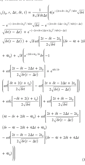
(Figure 2b), and the finite volume of the detected analyte reaching the detector window can be accounted for by afinite δt time (Figure 2d). Following the linear properties, we express these perturbations by a double integral:
∫ ∫
δ δ Δ = Δ δ δ −Δ − + A r t t t t t t A r x y x y ( , , , ; ) 1 1 ( , , ) d d x t t t t t t t 0 /2 /2 0 0 (2) The result of the integration, although being lengthy, can be readily obtained in a close form:δ π δ δ δ δ δ π δ δ δ δ π δ δ δ δ δ δ δ δ δ δ δ δ δ δ δ δ δ δ δ δ δ Δ = Δ − − − Δ + − Δ + − − − + + + − + − − Δ + − Δ + + + − + − Δ + − Δ + − + + + + − − + − + + − Δ − − Δ − − + Δ + − − − Δ − − Δ − + + Δ + δ δ δ δ δ δ − δ δ δ δ δ δ − + − − − + + − + − Δ − −Δ − + + Δ + −Δ − + L N MMM MMM MMM c e ddd ddd ddd f h ggg ggg ggg L N MMM MMM MM L N MMM MMM M c e ddd ddd ddd dd f h ggg ggg ggg gg L N MMM MMM M c e ddd ddd ddd f h ggg ggg ggg c e ddd ddd ddd dd f h ggg ggg ggg gg \ ^ ]]] ]]] ] c e ddd ddd ddd f h ggg ggg ggg \ ^ ]]] ]]] ] c e ddd ddd ddd f h ggg ggg ggg c e ddd ddd ddd dd f h ggg ggg ggg gg c e ddd ddd ddd dd f h ggg ggg ggg gg \ ^ ]]] ]]] ]] \ ^ ]]] ]]] ]]] A t r t t t t t rt rt r t t r t t t t t rt r t t t r t t t t r t t t t t rt t t t t r t t t t t rt t t t rt t r t t t t t t r t t r t t t t t t t t r t t r t t t t ( , , , , ) 1 8 4(e e e ( ) e ( ) ) erf 2 2 2 ( 4 2 4 ) e 1 erf 2 2 2 2 ( ) e erf 2( ) 2 erf 2 2 2 2 ( ) erfc 2( ) 2 erf 2 2 2 (4 2 4 ) erf 2 2 2 2 ( ) ( 4 2 4 4 ) erf 2 2 2 2 ( ) ( 4 2 4 4 ) x t t t rt t t t rt t t t t r t t t t t t r t t t t r t r 0 (2 2 ) /4 ( 2 2 ) /4 (2 2 2 ) /4 ( ) ( 2 2 2 ) /4 ( ) 0 0 2 4 / 0 4 / 0 0 0 0 0 0 0 0 0 02 02 02 02 0 (3)
Equation 3is adequate for interpreting Taylor dispersion, of either uniform particles or particles of moderate polydispersity, recorded with arbitrary injection and detection volumes and, thus, is not limited to small perturbations. By usingeq 3, it is straightforward to show that the residence time (t0) is
increasing withΔt/2 and the variance of the taylorgram (σ2) is increasing with (δt2 + Δt2)/12. Accordingly, the relative
accuracies regarding the residence time and variance areΔt/2t0
and (δt2 + Δt2)/(6t
0δr), respectively. Since the bias is
proportional to the square of the injection and detection times (i.e., volumes) and inversely proportional to residence time and particles size, the accuracy is decreasing with particle size at a given set of operational parameters. To deal with these systematic inaccuracies, it is most common to implement two
detection points, where one determined two variances (σ22,
σ12) and residence times (t2, t1). By using the differences in
variances and residence times determined from the recorded taylorgrams: πη σ σ = − − r k T Y t t 4 B 2 22 12 2 1 (4)
eq 4 aims at minimizing the bias resulting from a non-negligible pressure ramp and injection.21,22 However, this approach is inefficient when systematic errors owing to the practice of instrumentation are beyond small perturbations, which to the best of our knowledge, has remained untreated until now. To illustrate, let us consider the trivial case when the windows sizes are not exactly the same at both detection points. To impart resistance and mechanical strength, capillaries are coated with a protective polymer layer. This layer strongly absorbs in the UV−vis range and must be removed around the detection points. This is a very delicate step, with limited control over the exactness of the area. Accordingly, the biases will not be equal, and they will not cancel out in eq 4. While this might not stand out for larger particles and longer residence times, the characterization of small particles may suffer from this nonrecognized inaccuracy. To demonstrate the benefit of usingeq 3instead ofeq 1, we synthesized two batches of superparamagnetic iron oxide nanoparticles (SPIONs) and characterized their aqueous dispersions stabilized by citric acid (CA). The image analyses of TEM micrographs (Figure 3) show narrow size distributions with a radii of 6.0± 0.7 nm (mean ± STD) and 9.9 ± 0.6 nm, respectively.
To determine their diffusion coefficients and the corre-sponding hydrodynamic radii via Taylor dispersion, we recorded taylorgrams at two detection windows. Figure 4a shows two sets of representative data. The residence times were between 600 and 700 and 900−1000 s, respectively, and the ramping time was less than 5 s. As expected, the taylorgrams showed bimodality, where the narrower absorb-ance peak is attributed to the CA, and the broader peak is attributed to the SPIONs. Consequently, we, respectively, fitted the bimodal combinations of eq 1 and eq 3 to the taylorgrams (Figure 4b,c). The variances and residence times obtained via thefits were used to determine the particle radius via eq 4 and the Stokes−Einstein relationship, and Figure 5
shows thefinal results of the analyses.
Figure 3. TEM micrographs of the two citrate-stabilized SPIONs and the resulting distributions of the image analyses. The scale bar marks 50 nm.
Given the small dimensions and the nonzero imaginary part of the refractive index of the SPIONs, their optical extinction is dominated by absorption, and thus, the hydrodynamic radius measured by TDA is a volume-weighted average expressed by the raw moments of the size distribution: ⟨r4⟩/⟨r3⟩.7,9 The triangular bracket denote ensemble average, which is rapidly estimated from the TEM distribution. Accordingly, the radius
determined by Taylor dispersion is expected to be around 6.2 and 10.0 nm for the smaller and large SPIONs, respectively. Regarding the smaller SPIONs, the 0.99 confidence intervals of the radius determined via two-window measurements are, respectively, 5.5−6.4 nm when residence times and variances are determined viaeq 3and 3.9−5.3 nm when residence times and variances are determined via eq 1. The latter is entirely inconsistent with the value expected from the TEM analysis. Regarding the larger SPIONs, the 0.99 confidence intervals of the radius determined via two-window measurements are, respectively, 6.3−12.6 nm and 7.4−11.2 nm. Both intervals are consistent with the value expected from the TEM analysis. Therefore, as anticipated, the accuracy of an instrument with given operation parameters may be strongly dependent on the size of the particle.
To summarize, by treating Taylor dispersion as a linear time-invariant system, we extended the validity to larger injection and detection volumes increasing the quality of detection. This approach is new, promotes accuracy, and is dedicated to general-purpose instruments, where, while the operational parameters are not optimized for a given specific size, the versatility in sizing capacity is of high interest.
■
MATERIALS AND METHODSThe SPIONs were synthesized by thermal decomposition.23,24 Iron(III) chloride hexahydrate of ACS Reagent grade were purchased from Sigma-Aldrich, Merck KGaA, and Acros Organics. Sodium oleate (>97%) and tri-n-octylamine (>97%) were supplied by TCI Chemicals. Absolute ethanol (100%) and n-hexane (98%) of ACS Reagent grade were purchased from VWR Chemicals. Sigma-Aldrich supplied oleic acid (90%, technical grade), 1,2-dichlorobenzene (DCB, 99%) and n,n-dimethylformamide (DMF, ≥ 99.8%). Diethyl ether (ACS Reagent grade) and ammonium hydroxide solution (25%) were obtained from Honeywell Burdick & Jackson. Acetone (technical grade) was supplied by Reactolab SA. All chemicals were used as received. Each aqueous solution was prepared with deionized water received from a Milli-Q system (resistivity = 18.2 MΩ cm, Millipore AG). To transfer the SPIONs in aqueous solutions, a ligand exchange with citric acid (CA) was performed.25Colloidal stability was ensured by adding an excess of unbound CA (60 mg/mL) into the dispersions and subsequent adjustment to pH 7−8.26The CA (Sigma-Aldrich, ACS reagent,≥99.5%) was dissolved in Milli-Q water to obtain a 60 mg/mL solution.
For transmission electron microscopy (TEM), diluted samples were dropcasted onto 300 mesh carbon membrane-coated copper grids following a procedure described else-where.27TEM experiments were carried out on a FEI Tecnai Spirit operating at a voltage of 120 kV and equipped with a side-mounted Veleta CCD camera (Olympus). The core diameters of the nanoparticles were determined using an automatized size distribution analysis macro in ImageJ (v1.50i).
Taylor dispersion spectra were collected by a capillary electrophoresis injection system (Prince 560 CE Autosampler, Prince Technologies B.V.) using a fused silica capillary (74.5 μm inner diameter, Polymicro Technologies, Phoenix, AZ) at constant temperature of 25°C. The running buffer was Milli-Q-water. Analytes with a volume of approximately 112 nL were injected for 12 s at 200 mbar (ramp time, 4.8 s). The pressure of 90 mbar (ramp time, 3 s) drove the samples through the capillary with a mean velocity of around 1 mm/s. In our Figure 4. (a) Two sets of taylorgrams of the smaller SPIONs shown
inFigure 3(on the left). The repeatability is excellent, and thus, the taylorgrams are shifted vertically for the sake of visibility. The taylorgrams show bimodality, where the narrower absorbance peak is attributed to the CA, and the broader peak is attributed to the SPIONs. (b) The bestfit ofeq 1is drawn in dashed orange, and the bestfit ofeq 3is drawn in blue. The light blue curve shows the ideal experimental taylorgram corresponding to infinitely small volumes, drawn via the bestfiteq 3. (c) The decomposition of the best bimodal fits ofeq 1(dashed orange) andeq 3(blue).
Figure 5. Residence times and variances obtained viaeqs 1and3(in orange and blue, respectively) for the (a) smaller and (b) larger SPIONs. To compare the slopes determined viaeq 4, the blue line is shifted near to the orange line. The small yet relevant deviation in the slope in the case of the small SPIONs clearly shows the result of bias originating fromeq 1.
experiments, the duration of the pressure ramp was negligible compared to the residence times, and accordingly we did not need to apply any correction for this small perturbation.21The full length of the capillary was 145.5 cm, equipped with two detection windows with a width of 1 cm each. The distance to the first and second window was 72.5 and 104.5 cm, respectively. Absorbance was recorded by an ActiPix D100 UV−vis area imaging detector (Paraytec, York, U.K., 20 Hz sampling rate) using a band-pass filter (520 nm center wavelength, 10 nm fwhm) coupled with a neutral density filter (10% transmission, Edmund Optics, York, U.K.). The detector corrects the intensity values for dark current, controls the intensity of illumination, and performs the background measurement on the respective running buffer before each run. The extinction of the particles is expected to be collected in the linear range of the detector throughout the measurements, and the resulting absorbance is determined by taking into account variations in the illumination, solvent backgrounds, and dark current. To analyze the taylorgrams, routines were coded by using Mathematica (version 11.3, Wolfram Language, Wolfram Research, Inc., Champaign, IL). Tofit our model against the experimental data, we used an unconstrained nonlinear model fit. The details along with a complete set of results are presented in theSupporting Information.
■
ASSOCIATED CONTENT S*
Supporting InformationThe Supporting Information is available
■
AUTHOR INFORMATION Corresponding Author *E-mail:[email protected]. ORCID Alke Petri-Fink:0000-0003-3952-7849 Sandor Balog:0000-0002-4847-9845 Author ContributionsP.L. synthesized the particles, collected the Taylor dispersion data, and collected and analyzed the TEM micrographs. A.P-F. supervised P.L. S.B. conceived the project, developed the analytical approach, and analyzed the Taylor dispersion data. S.B. wrote the manuscript with contribution from the other authors.
Notes
The authors declare no competingfinancial interest.
■
ACKNOWLEDGMENTSThe authors are grateful for the financial support of the Adolphe Merkle Foundation, the University of Fribourg, and the Swiss National Science Foundation through the National Centre of Competence in Research Bio-Inspired Materials and the Grant SNF No. 159803 (P.L. and A.P.-F.).
■
REFERENCES(1) Taylor, G. Proc. R. Soc. London, Ser. A 1953, 219, 186−203. (2) Taylor, G. Proc. R. Soc. London, Ser. A 1954, 225, 473−477. (3) Aris, R. Proc. R. Soc. London, Ser. A 1956, 235, 67−77. (4) Belongia, B. M.; Baygents, J. C. J. Colloid Interface Sci. 1997, 195, 19−31.
(5) Pyell, U.; Jalil, A. H.; Pfeiffer, C.; Pelaz, B.; Parak, W. J. J. Colloid Interface Sci. 2015, 450, 288−300.
(6) Pyell, U.; Jalil, A. H.; Urban, D. A.; Pfeiffer, C.; Pelaz, B.; Parak, W. J. J. Colloid Interface Sci. 2015, 457, 131−140.
(7) Balog, S.; Urban, D. A.; Milosevic, A. M.; Crippa, F.; Rothen-Rutishauser, B.; Petri-Fink, A. J. Nanopart. Res. 2017, 19, 287.
(8) Fichtner, A.; Jalil, A.; Pyell, U. Langmuir 2017, 33, 2325−2339. (9) Balog, S. Anal. Chem. 2018, 90, 4258−4262.
(10) Urban, D. A.; Milosevic, A. M.; Bossert, D.; Crippa, F.; Moore, T. L.; Geers, C.; Balog, S.; Rothen-Rutishauser, B.; Petri-Fink, A. Colloid and Interface Science Communications 2018, 22, 29−33.
(11) Oukacine, F.; Gèze, A.; Choisnard, L.; Putaux, J.-L.; Stahl, J.-P.; Peyrin, E. Anal. Chem. 2018, 90, 2493−2500.
(12) d’Orlyé, F.; Varenne, A.; Gareil, P. Journal of Chromatography A 2008, 1204, 226−232.
(13) Einstein, A. Ann. Phys. 1905, 322, 549−560. (14) Einstein, A. Ann. Phys. 1906, 324, 289−306. (15) Einstein, A. Ann. Phys. 1911, 339, 591−592.
(16) Cottet, H.; Biron, J.-P.; Martin, M. Analyst 2014, 139, 3552− 3562.
(17) Alizadeh, A.; Nieto de Castro, C. A.; Wakeham, W. A. Int. J. Thermophys. 1980, 1, 243−284.
(18) Chamieh, J.; Leclercq, L.; Martin, M.; Slaoui, S.; Jensen, H.; Østergaard, J.; Cottet, H. Anal. Chem. 2017, 89, 13487−13493.
(19) Rao, K. D. Signals and Systems; Birkhäuser Basel, 2018. (20) Gupta, V. K.; Bhattacharya, R. N. Water Resour. Res. 1983, 19, 945−951.
(21) Sharma, U.; Gleason, N. J.; Carbeck, J. D. Anal. Chem. 2005, 77, 806−813.
(22) Chamieh, J.; Cottet, H. Journal of Chromatography A 2012, 1241, 123−127.
(23) Park, J.; An, K.; Hwang, Y.; Park, J.-G.; Noh, H.-J.; Kim, J.-Y.; Park, J.-H.; Hwang, N.-M.; Hyeon, T. Nat. Mater. 2004, 3, 891.
(24) Hou, Y.; Xu, Z.; Sun, S. Angew. Chem., Int. Ed. 2007, 46, 6329− 6332.
(25) Lattuada, M.; Hatton, T. A. Langmuir 2007, 23, 2158−2168. (26) de Sousa, M. E.; Fernández van Raap, M. B.; Rivas, P. C.; Mendoza Zélis, P.; Girardin, P.; Pasquevich, G. A.; Alessandrini, J. L.; Muraca, D.; Sánchez, F. H. J. Phys. Chem. C 2013, 117, 5436−5445. (27) Michen, B.; Geers, C.; Vanhecke, D.; Endes, C.; Rothen-Rutishauser, B.; Balog, S.; Petri-Fink, A. Sci. Rep. 2015, 5, 9793.