Sensitivity checks for the local average treatment effect

(1)

Sensitivity checks for the local average treatment effect

Martin Huber

March 13, 2014

University of St. Gallen, Dept. of Economics

Abstract: The nonparametric identification of the local average treatment effect (LATE) hinges on the satisfaction of three instrumental variable assumptions: (1) Unconfounded assignment of the instrument, (2) no average direct effect of the instrument on the outcome within compliance types (exclusion restric-tion), and (3) weak monotonicity of the treatment in the instrument. While (1) often appears plausible in experiments when using randomization as instrument for actual participation, (2) and (3) may be con-troversial. For this reason, this paper proposes easily implementable sensitivity checks to assess the ro-bustness of the LATE to deviations from either the exclusion restriction or monotonicity. An empirical illustration based on female labor supply data is also provided.

Keywords: instrumental variable, treatment effects, LATE, sensitivity analysis. JEL classification: C21, C26.

I have benefitted from comments by an anonymous referee. Financial support from the Swiss National Sci-ence Foundation grant PBSGP1 138770 is gratefully acknowledged. Address for correspondSci-ence: Martin Huber (martin.huber@unisg.ch), SEW, University of St. Gallen, Varnb¨uelstrasse 14, 9000 St. Gallen, Switzerland.

(2)

1 Identifying the LATE

Suppose we are interested in the effect of a binary endogenous treatment D on an outcome Y and have available a binary instrument Z. Denote by D(z) the potential treatment state for instrument Z = z and by Y (d, z) the potential outcome for treatment D = d and instrument Z = z. As discussed in Angrist, Imbens, and Rubin (1996), the population can be categorized into four types (denoted by T ∈ {a, c, d, n}), depending on how the treatment reacts to the instrument: compliers (D(1) = 1, D(0) = 0), always takers (D(1) = 1, D(0) = 1), never takers (D(1) = 0, D(0) = 0), and defiers (D(1) = 0, D(0) = 1). However, the types are not identified from the data, because any observed treatment-instrument-combination either reveals D(1) or D(0), so that any observation may belong to one of two candidate types. Under the following assumptions, the local average treatment effect (LATE) on compliers is nevertheless identified. Assumption 1:

Pr(T = t|Z = 1) = Pr(T = t|Z = 0) for t ∈ {a, c, d, n} (unconfounded type).

Assumption 1 states that the instrument is assigned independently of the types (as in randomized trials) so that the share of any type conditional on the instrument is equal to its unconditional proportion. Therefore, any conditional treatment probability consists of two type proportions:

P1|1= πa+ πc, P0|1= πd+ πn, P1|0 = πa+ πd, P0|0= πc+ πn, (1)

where πt ≡ Pr(T = t), t ∈ {a, c, n}, and Pd|z ≡ Pr(D = d|Z = z). Similarly, each of the four

observed conditional means E(Y |D = d, Z = z) is a mixture or weighted average of the mean potential outcomes of two types conditional on the instrument (denoted by E(Y (d, z)|T = t, Z = z)), where the weights depend on the relative proportions:

(3)

Assumption 2:

E(Y (d, 1)|T = t, Z = 1) = E(Y (d, 0)|T = t, Z = 0) = E(Y (d)|T = t) for d ∈ {0, 1} and t ∈ {a, c, d, n} (mean exclusion restriction),

Assumption 2 states that the instrument does not affect the mean potential outcomes within any subpopulation, e.g. E(Y (1, 1)|T = a, Z = 1) = E(Y (1, 0)|T = a, Z = 0) = E(Y (1)|T = a). Assumption 3:

Pr(D(1) ≥ D(0)) = 1, Pr(D(1) > D(0)) > 0 (monotonicity),

Assumption 3 rules out defiers (type d), but implies the presence of compliers (type c).

As defiers do not exist, the shares of the remaining types in (1) are identified by P_0|1 = πn,

P1|0 = πa, P1|1− P1|0 = P0|0− P0|1 = πc. Furthermore, the mean potential outcomes of always

takers under treatment and never takers under non-treatment are point identified, because (3) simplifies to E(Y |D = 1, Z = 0) = E(Y (1)|T = a) and (5) to E(Y |D = 0, Z = 1) = E(Y (0)|T = n). Finally, plugging E(Y |D = 1, Z = 0) and E(Y |D = 0, Z = 1) into (2) and (4) allows solving the equations for the mean potential outcomes of compliers under either treatment state:

E(Y (1)|T = c) = P1|1· E(Y |D = 1, Z = 1) − P1|0· E(Y |D = 1, Z = 0) P1|1− P1|0

,

E(Y (0)|T = c) = P0|0· E(Y |D = 0, Z = 0) − P0|1· E(Y |D = 0, Z = 1) P1|1− P1|0

. (6)

The difference of the latter gives the LATE and can be shown to simplify to the probability limit of the Wald estimator _{E(D|Z=1)−E(D|Z=0)}E(Y |Z=1)−E(Y |Z=0).

2 Sensitivity analysis

We subsequently propose novel sensitivity checks for the robustness of the LATE under deviations from either Assumption 2 (exclusion restriction) or 3 (monotonicity), whereas Assumption 1 is assumed to be satisfied (which appears plausible in randomized trials). It is important to note that we separately consider violations of one assumption while maintaining the respective other

(4)

one (rather than assuming joint violations of Assumptions 2 and 3).1 This work is related to the growing literature on modelling violations of the exclusion restriction (see for instance Altonji, Elder, and Taber (2005), Choi and Lee (2012), Conley, Hansen, and Rossi (2012), and Nevo and Rosen (2012) for parametric approaches and Flores and Flores-Lagunes (2013) and Mealli and Pacini (2013) for nonparametric bounds) or of monotonicity (see Richardson and Robins (2010)).

A violation of the exclusion restriction occurs if the instrument has a non-zero average direct effect on the types’ mean potential outcomes. Then, the conditional mean outcomes E(Y |D = 1, Z = 1) and E(Y |D = 0, Z = 1) not only consist of the (mixtures of) mean potential outcomes of the types, but also of the direct effect (which is absent under Z = 0). We therefore add the potentially heterogenous average direct effects of Z to the mean potential outcomes of the compliers, always takers, and never takers, which are denoted by γc, γa, and γn:

For instance, γc = E(Y (1)|T = c, Z = 1) − E(Y (1)|T = c, Z = 0), because E(Y (1)|T = c, Z =

1) 6= E(Y (1)|T = c, Z = 0) if Assumption 2 does not hold. Using (7) in (6) gives

E(Y (1)|T = c) = P1|1· E(Y |D = 1, Z = 1) − P1|0· (E(Y |D = 1, Z = 0) + γa) P1|1− P1|0

− γc,

E(Y (0)|T = c) = P0|0· E(Y |D = 0, Z = 0) − P0|1· (E(Y |D = 0, Z = 1) − γn) P1|1− P1|0

, (8)

which are the bias-corrected mean potential outcomes among compliers. Therefore, the LATE is

LATE = E(Y |Z = 1) − E(Y |Z = 0) − P1|0· γa− P0|1· γn P1|1− P1|0

− γc. (9)

If we have no prior belief on whether such a heterogeneity exists, we may consider homogeneous

1

Note that sensitivity analysis under a joint violation of Assumptions 2 and 3 would need to account for interactions between the parameters gauging deviations from either Assumption 2 or Assumption 3 suggested further below, which is out of the scope of this note.

(5)

direct effects across types so that γa = γn= γc= γ. For this special case, (9) simplifies to

LATE = E(Y |Z = 1) − E(Y |Z = 0) − γ P1|1− P1|0

. (10)

This corresponds to the probability limit of the slope coefficient in TSLS when regressing D on one and Z in the first stage and Y − Zγ on one and the first stage prediction of D in the second stage, as considered in Conley, Hansen, and Rossi (2012). Therefore, if γ is homogeneous across types, our identification result is numerically equivalent, however, the interpretation differs: Whereas we confine ourselves to the LATE, the parametric restrictions in Conley, Hansen, and Rossi (2012) imply a constant individual (and thus, average) treatment effect. Under heterogenous γa, γn, γc,

the LATE no longer simplifies to (10) or the probability limit of TSLS. If heterogeneity should be permitted, sensitivity analysis based on parametric models therefore appears less attractive than relying on the mean potential outcome framework advocated here. On the other hand, it has to be acknowledged that our sensitivity analysis only applies to binary treatments (while extending our method to non-binary instruments would not be difficult), whereas parametric approaches also allow for more general treatment variables.

As a second contribution, we consider a violation of monotonicity (Assumption 3), which entails two issues. Firstly, the shares of the compliers or any other type are no longer point identified, because without assuming monotonicity, e.g. P1|1− P1|0= πc− πd⇔ P1|1− P1|0+ πd=

πc. Secondly, the mean potential outcomes of the always and never takers are no longer identified,

which is required for the point identification of the compliers’ mean potential outcomes under treatment and non-treatment. The reason is that E(Y |D = 1, Z = 0) = E(Y (1)|T = a) + E(Y (1)|T = d) and E(Y |D = 0, Z = 1) = E(Y (0)|T = n) + E(Y (0)|T = d) are mixtures of the mean potential outcomes of defiers and always or never takers, respectively. Therefore, the parameters to be manipulated in sensitivity checks are the share of defiers (which deterministically sets the share of any other type) as well as the mean potential outcomes of the always takers and compliers under treatment and of the never takers and compliers under non-treatment.

(6)

Concerning the latter problem, note that one may express the potential outcome of one pop-ulation as proportion of that of the other poppop-ulation in the respective mixture. Let E(Y (1)|T = a) = ρaE(Y (1)|T = c) with the ratio ρa = E(Y (1)|T = a)/E(Y (1)|T = c) and E(Y (0)|T = n) =

ρnE(Y (0)|T = c) with the ratio ρn= E(Y (0)|T = n)/E(Y (0)|T = c). It follows that (2) and (4)

can be rewritten in terms of the mean potential outcomes of the compliers only:

Solving for the potential outcomes of the compliers yields

E(Y (1)|T = c) = (πa+ πc) · E(Y |D = 1, Z = 1) ρaπa+ πc

, E(Y (0)|T = c) = (πn+ πc) · E(Y |D = 0, Z = 0) ρnπn+ πc

.(12)

In the sensitivity analysis, ρa, ρn have to be varied over a plausible range. E.g., if ρa = 1, then

E(Y |D = 1, Z = 1) = E(Y (1)|T = c), implying that the mean potential outcomes of always takers and compliers are equal. A natural starting point for choosing ρa and ρn is

φa= E(Y |D = 1, Z = 0) P1|1·E(Y |D=1,Z=1)−P1|0·E(Y |D=1,Z=0) P1|1−P1|0 , φn= E(Y |D = 0, Z = 1) P0|0·E(Y |D=0,Z=0)−P0|1·E(Y |D=0,Z=1) P1|1−P1|0 , (13)

where φa and φn are the ratios of the respective quantities in (6) if monotonicity (along with the

other assumptions) is satisfied. Therefore, under moderate deviations from monotonicity, φaand

φn are most likely not too different from the actual ratios ρa and ρn. By setting ρa = βaφa and

ρn= βnφn we can use any βa> 0, βn> 0 different to unity to gauge the supposed violation as a

function of the empirically advised outcome ratios.

On top of βa, βn(or ρa, ρndirectly), we also need to incorporate uncertainty about the defier

πn+ πc= P0|0 in (12) as well as ρa= βaφa and ρn= βnφn, we obtain

(7)

Sensitivity analysis w.r.t. to non-monotonicity therefore requires varying three parameters, namely βa, βn, (or ρa, ρn) and πd, over a plausible range.

3 Empirical illustration

Angrist and Evans (1998) aim at assessing the effect of fertility on female labor supply using the US Census Public Use Micro Samples (PUMS). As fertility and labor supply are most likely endogenous, the authors use the sex ratio of the first two children as instrument for fertility (to get at least one more child). The supposedly randomly assigned sex of children should not directly affect labor supply, while monotonicity is motivated by US parents’ general preference for mixed sex siblings. However, as Rosenzweig and Wolpin (2000) argue, having mixed sex siblings may violate the exclusion restriction by directly affecting both the marginal utility of leisure and child rearing costs and, thus, labor supply. Also the satisfaction of monotonicity for every parent in the population appears questionable in the light of empirical evidence on the preference for boys in some cultures, see for instance Lee (2008). We separately investigate deviations from the mean exclusion restriction and monotonicity, considering the 1980 wave of the PUMS data. Treatment D indicates whether a mother has three or more children (158,751 observations) or just two (236,089). Z is one if the first two children have the same sex (199,548) and zero otherwise (195,292). The outcome Y is hours worked per week. The first stage regression of D on Z suggests that same sex increases the probability of a third child by roughly 6 percentage points. The Wald estimator predicts a reduction of 5.187 hours among compliers and is highly significant (robust standard error: 1.006). TSLS conditioning on additional covariates (age, education, marital status, race, year of first birth) gives a similar effect of -4.545 hours (robust standard error: 0.959).

Concerning potential violations of Assumption 2, increased costs of mixed sex siblings (e.g. no room-sharing or hand-me-downs) may induce women to provide more labor to increase household income. On the other hand, mixed sex siblings may be more time consuming due to sex-specific

(8)

activities so that females may substitute time at work by time with children. We assume the cost argument to (weakly) outweigh the time substitution argument, implying γa, γc, γn ≥ 0.

Furthermore, we suspect the average direct effect to be largest for the never takers, who arguably have the highest valuation of work life and earnings due to their choice not to have further children irrespective of the sex ratio. Accordingly, the always takers are supposed to have the lowest direct effect due to their arguably high preference for family life. This suggests γn > γc > γa. Table

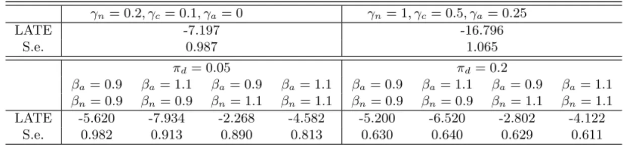
1 (upper panel) reports the LATE estimates for two different choices of γn, γc, γa, including

bootstrap standard errors (based on 999 bootstrap draws). Due to the small first stage, the results are quite sensitive to violations of Assumption 2. Already moderate average direct effects on never takers and compliers (γn = 0.2, γc = 0.1, γa = 0) decrease the LATE based on Wald

estimation considerably by roughly 2 to -7.197 hours per week. Under more severe direct effects on all subpopulations (γn= 1, γc= 0.5, γa= 0.25)2 the negative LATE is even much stronger.

The estimates of φa and φn are 1.11 and 1.02, respectively. This suggests that if

Assump-tions 1-3 hold, always takers work more hours than compliers under treatment, while never takers and compliers are fairly comparable under non-treatment. Table 1 (lower panel) gives the LATE estimates under a violation of Assumption 3 using various combinations of βa, βn, and πd.

Specif-ically, βa and βn vary between 0.9 and 1.1, implying moderate deviations from the empirically

advised potential outcome ratios. πd is set to 0.05 and 0.2, in order to investigate the sensitivity

of the results to both small and more substantial shares of defiers (which may exist if the findings in Lee (2008) carry over to some socio-economic groups in the US). The estimates suggest that the negativity of the labor supply effect of fertility is robust to the violations of monotonicity considered, as all LATEs remain significantly below zero.3

2

Even larger direct effects appear unreasonable as γn = 1 already amounts to more than 5% of the average

working hours per week observed in the sample (18.798 hours) and more than 20% of the absolute value of the LATE estimate under the satisfaction of Assumptions 1-3 (-5.187 hours).

3_{Note that the LATE ceteris paribus increases in β}

n and decreases in βa. E.g. for πd = 0.05 and βn = 1.1,

the LATE is significantly negative at the 5% level when setting βa to 0.85 or larger values (one-sided hypothesis

(9)

Table 1: Violations of the exclusion restriction (upper panel) or monotonicity (lower panel) γn= 0.2, γc= 0.1, γa= 0 γn= 1, γc= 0.5, γa= 0.25 LATE -7.197 -16.796 S.e. 0.987 1.065 πd= 0.05 πd= 0.2 βa= 0.9 βa= 1.1 βa= 0.9 βa= 1.1 βa= 0.9 βa= 1.1 βa= 0.9 βa= 1.1 βn= 0.9 βn= 0.9 βn= 1.1 βn= 1.1 βn= 0.9 βn= 0.9 βn= 1.1 βn= 1.1 LATE -5.620 -7.934 -2.268 -4.582 -5.200 -6.520 -2.802 -4.122 S.e. 0.982 0.913 0.890 0.813 0.630 0.640 0.629 0.611

Note: S.e.: Bootstrap standard errors based on 999 bootstrap draws.

References

Altonji, J. G., T. E. Elder,andC. R. Taber (2005): “An Evaluation of Instrumental Variable Strategies for Estimating the Effects of Catholic Schooling,” The Journal of Human Resources, 40, 791–821.

Angrist, J.,andW. Evans (1998): “Children and their parents labor supply: Evidence from exogeneous variation in family size,” American Economic Review, 88, 450–477.

Angrist, J., G. Imbens,andD. Rubin (1996): “Identification of Causal Effects using Instrumental Variables,” Journal of American Statistical Association, 91, 444–472.

Choi, J.-y.,and M.-j. Lee (2012): “Bounding endogenous regressor coefficients using moment inequalities and generalized instruments,” Statistica Neerlandica, 66, 161–182.

Conley, T. G., C. B. Hansen, and P. E. Rossi (2012): “Plausibly Exogenous,” Review of Economics and Statistics, 94, 260–272.

Flores, C. A.,andA. Flores-Lagunes (2013): “Partial Identification of Local Average Treatment Effects with an Invalid Instrument,” Journal of Business & Economic Statistics, 31, 534–545.

Lee, J. (2008): “Sibling size and investment in childrens education: an Asian instrument,” Journal of Population Economics, 21, 855–875.

Mealli, F.,andB. Pacini (2013): “Using secondary outcomes and covariates to sharpen inference in instrumental variable settings,” Journal of the American Statistical Association, 108, 1120–1131.

Nevo, A., and A. M. Rosen (2012): “Identification with Imperfect Instruments,” Review of Economics and Statistics, 94, 659–671.

Richardson, T. S.,andJ. M. Robins (2010): “Analysis of the Binary Instrumental Variable Model,” in Heuris-tics, probability and causality: a tribute to Judea Pearl, ed. by R. Dechter, H. Geffner,andJ. Y. Halpern, pp. 415–440, London, UK. College Publications.

(10)

Rosenzweig, M. R., and K. I. Wolpin (2000): “Natural ”Natural Experiments” in Economics,” Journal of Economic Literature, 38, 827–874.