HAL Id: hal-00117348
https://hal.archives-ouvertes.fr/hal-00117348
Preprint submitted on 13 Dec 2006HAL is a multi-disciplinary open access
archive for the deposit and dissemination of sci-entific research documents, whether they are pub-lished or not. The documents may come from teaching and research institutions in France or abroad, or from public or private research centers.
L’archive ouverte pluridisciplinaire HAL, est destinée au dépôt et à la diffusion de documents scientifiques de niveau recherche, publiés ou non, émanant des établissements d’enseignement et de recherche français ou étrangers, des laboratoires publics ou privés.
The Sumatran earthquake impact on Earth Rotation
from satellite gravimetric measurements
Christian Bizouard, Lucia Seoane
To cite this version:
Christian Bizouard, Lucia Seoane. The Sumatran earthquake impact on Earth Rotation from satellite gravimetric measurements. 2006. �hal-00117348�
The Sumatran earthquake impact on Earth Rotation from
satellite gravimetric measurements
Christian Bizouard
Luc´ıa Seoane Corral
Paris Observatory, 61 avenue de l’Observatoire, 75014 Paris,
Tel.: +0033140512335
christian.bizouard@obspm.fr
september 2006
Abstract
From the satellite gravity field measurements (mission GRACE and LAGEOS) we computed the changes in inertia moments of the Earth, which have followed the gigantic Sumatra Earthquake of December 26, 2004. Our approach is based upon the geoid height variations, which has been caused by the Earthquake. According to those gravimetric data, the pole was shifted up to 2 mas towards 90oEast and the length of day dropped up
to -5 µs. The phase obtained for the pole shift contradicts that one derived from seismic model.
Keywords : Earth rotation Sumatra Earthquake Gravity field variation GRACE
1
Introduction
Whereas the influence of earthquakes on Earth rotation is a recurrent theme since the sixties, nothing has been ever observed. The gigantic Earthquake, that took place on 2004 December 26 at 00h 58min 51s UTC, about 200 km from the western coast of northern Sumatra (epicenter of latitude 3.298◦ and longitude 95.778◦), has constituted an opportunity for recording a possible
effect. Indeed its magnitude on the Richter scale reached at least m = 9, that makes it the third or forth biggest Earthquake ever recorded after those of Chile (1960, m = 9.5), Alaska (1964, m = 9.2), Kamchatka (1959, m = 9). The earthquake occurred as thrust-faulting on the interface of the India plate and the Burma microplate. In a period of minutes, the faulting released elastic strains that had accumulated for centuries from ongoing subduction of the India plate beneath the overriding Burma microplate. The ground over 1000 km fault was displaced in average by about 11 m. Probably as well shaken as the Earth, some geophysicists, relieved by journalists, claimed in the following hours of the catastrophe, that a sudden polar shift had been observed. In the same time we began our investigation.
Until now the unique way for estimating the influence of the Earthquakes on the Earth rotation was to model the seismic displacement according to the seismic parameters, to derive the changes in Earth inertia moments, and in virtue of the angular momentum balance the rotational effect itself. We had performed this study by applying the Dahlen model (1973), and concluded that the giant Sumatra Earthquakes produced polar shift of about 1-3 cm, too small quantity to be distinguished from daily polar motion associated with atmospheric, oceanic and hydrological excitation (Bizouard, 2005). By applying their own model, Gross and Chao (2006) reached a similar conclusion and estimated that the lenght of day (LOD) should have decreased by a few µs (far below the observed accuracy of 20 µs). For the largest earthquake ever recorded (Chile, 1960) the displacement would have reached 30 cm, and could have been noticed in polar motion whether this later one has been measured by means of modern geodetic techniques.
But the recent observations of the Earth’s gravity field by the mission GRACE (Gravity Recovery and Climate Experiment), begun in 2002, bring a new approach for tackling this problem. Looking at the variations of geoid height around December 26 2004, as measured by GRACE, Loyer (2006), member of the french team GRGS (”Groupement de Recherche pour la G´eod´esie Spatiale”), noticed a depression of about 1 cm in Indonesia (Fig. 1)-A. From that drop in geoid height the redistribution of mass caused by this earthquake could be tracked and the associated rotational effect could be derived.
Our paper is devoted to this challenge. In section 2 a short description of the GRACE data is given. In section 3 we confirm that the lowering of the geoid was indeed caused by this earthquake. In section 4 the Sumatran rotational effect is computed.
2
Geoid height variation from GRACE and LAGEOS
observations
The satellite mission GRACE, always in progress, aims at the very precise determination of the Earth’s gravity field, especially of its temporal variations. By combining the GRACE ob-servations to those of the satellite LAGEOS (mostly reliable for the low degrees of the geopo-tential), the GRGS team (France) produced a solution, which acts as international standard today (Biancale et al., 2005). This solution, extending at the present time over 3 years (July 2002-September 2005), regularly lengthens thanks to the treatment of the new observations. It consists in a static part, of which the spherical harmonic development extends up to degree 150, and a variable part, of which the spherical harmonic development extends up to degree 50. For the variable part the Stokes coefficients are given with 10 days step (July 2002-September 2005). The variable gravity field is also translated into 105 1o× 1o latitude-longitude grids of
the geoid height (referred to the reference ellipsoid) with a 10 days step. The spatial resolution of this geoid grids reaches 3.2o. It should be noticed that the variable part was freed from well
modeled variations :
• effect of terrestrial tides : Convention 2003 of the IERS (International Earth Rotation and Reference Systems Service).
the ECMWF (European Center of Meteorological Weather Forecast) provided every 6 hours / oceanic barotropic model ”MOG2D”
• effect of the oceanic tides : model ”FES-2004” of the LEGOS (Midi-Pyr´en´es Observatory). The observed variations mostly reflects hydrological effect and non-modeled oceanic circulation.
Precision. The normalised Stokes coefficients ¯Clm and ¯Slm are given with a precision below
10−11. The grids of geoid height are not provided with their uncertainties. By carrying out
independent analysis, Wahr et al.. (2006) confer to them errors from σ = 0.2 mm (spatial frequencies associated with Stokes coefficients of degrees 10-20) to σ = 0.7 mm (degree 40).
Link with the inertia moments of the Earth. In the terrestrial frame Oxyz, by assuming
a biaxial Earth the inertia matrix takes the form :
I= I11 I12 I13 I12 I22 I23 I13 I23 I33 = A + c11 c12 c13 c12 A + c22 c23 c13 c23 C + c33 (1)
where cij with i, j = 1, 2, 3 are the increments of inertia moment associated with the mass
distribution at a given time.
The coefficients of interest are I13, I23 et I33 or their increments. They are directly linked
to the Stokes coefficients (Clm, Slm) of degree 2 by the relations (see e.g. Lambeck, 1980) :
I13 = −MeRe2C21 (2) I23 = −MeRe2S21 (3) I33 = 1 3T r(I) − 2 3MeR 2 eC20 (4)
where T r(I) = I11 + I22 + I33. On the reasonable assumption that the mechanical system
preserved its mass, it is showed that the trace remains constant (Rochester & Smylie 1974). Therefore, a redistribution of masses causing a variation ∆C20 of the Stoke coefficient C20
induces the axial inertia moment increment : ∆I33 = −
2 3MeR
2
e∆C20 (5)
3
”Sumatran effect” on geoid height
First glance at the geoid height. In a premonitory study published a few month before the catastrophe, Mikhailov et al. (1994) announced the possibility to detect huge earthquake by GRACE. In a first approximation a seism produces a permanent redistribution of masses. Its duration (approximately 10 minutes) is negligible in comparison with the time sampling of the geoid grid, given every 10 days by stacking the measurements over one month. One
−150 −100 −50 0 50 100 150 −90 −60 −30 0 30 60 90 Geoid height (cm) −1 −0.5 0 0.5 (A) −150 −100 −50 0 50 100 150 −90 −60 −30 0 30 60 90 Geoid height (cm) −0.5 −0.4 −0.3 −0.2 −0.1 0 0.1 0.2 0.3 0.4 0.5 (A)
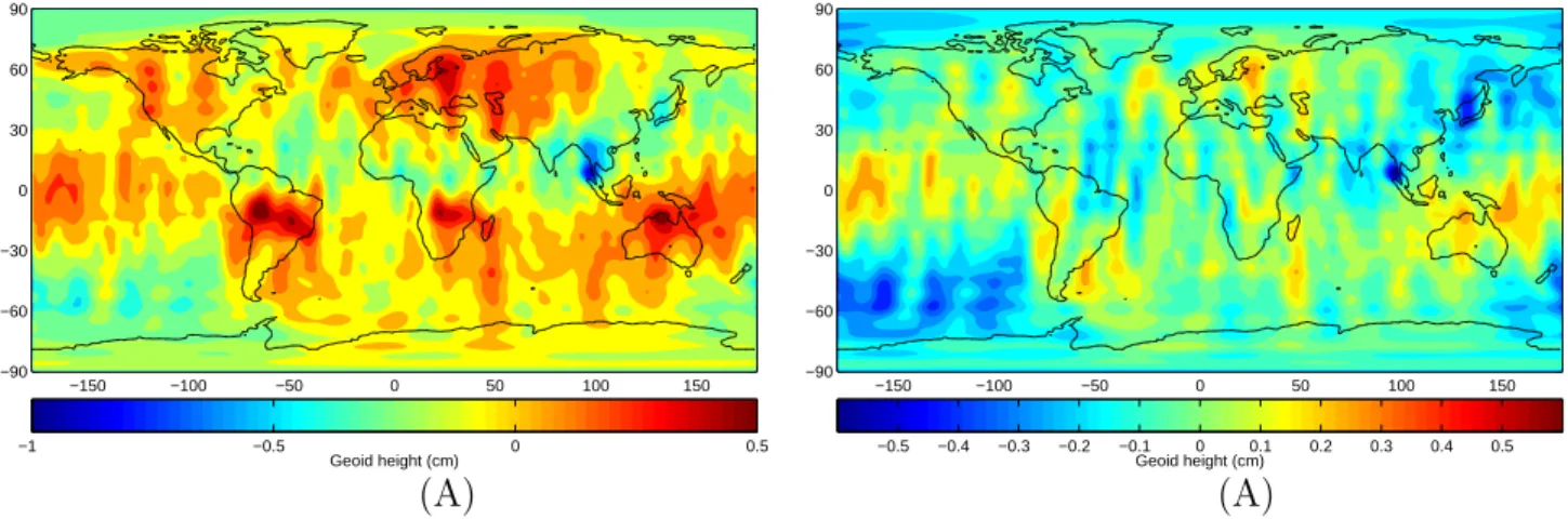
Figure 1: Difference of the monthly geoid grids preceding and following the seism of Sumatra (A) ; freed from seasonal variation (B).
thus expects that, over the zone affected by the seism, the geoid height has undergone quasi-permanent offsets. Indeed, by subtracting the monthly grid preceding the Sumatran seism (from Novembrer 25, 2004 to December 24,2004) to the one following it (from December 25, 2004 to January 23, 2005) Loyer (2006) noticed an obvious anomaly on the area of Sumatra. In this zone the geoid dropped from almost 1 cm, as attested by Fig. 1.
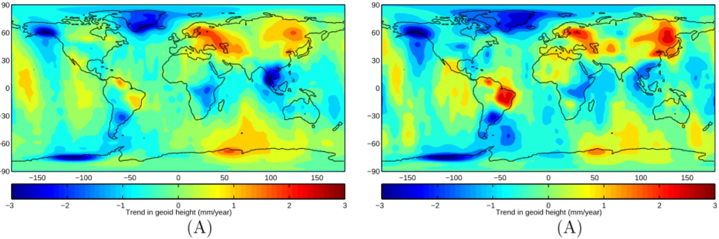
Let us see whether some trend become apparent in the geoid height over the whole data set. This one is estimated as a linear term for each point of the grid. The result displayed on Fig. 2-A confirms a lowering on the zone of Sumatra up to 3 mm/year. This trend is clearly linked with the event of December 26, 2004, because such a trend, estimated over the period before the seism, as showed by Fig. 2-B almost disappears.
We can also see significant reduction of geoid height on Greenland, Alaska and Antarctic. As the equation (9) justifies it (see there-after) the linear trend in these area is connected with the decrease of the geopotential, that we can interpret by a local loss of mass produced by the continental ice melting. This could testify the global warning and its impact on polar ice. For more detail on the quantity of melted mass, one will refer to the studies of Velicogna et al. (2005).
From the geoid height, we shall try to determine the variation of the coefficients ∆C21 and
∆S21associated with the zone of the seism and in return the variations of the moments of inertia
∆I13 and ∆I23 according to the equations (2), (3), (5) and their effect on terrestrial rotation.
Hereafter one describes the steps to be followed to isolate and estimate “the Sumatran effect” starting from the geoid height. The calculation and figures were carried out by programming under MATLAB.
Removing of the seasonal variations in the geoid height. The geoid undergoes seasonal variations, at the level of 1 cm over Indonesia, which could produce artifacts. For that reason they have been removed by least square procedure.
−150 −100 −50 0 50 100 150 −90 −60 −30 0 30 60 90
Trend in geoid height (mm/year)
−3 −2 −1 0 1 2 3 (A) −150 −100 −50 0 50 100 150 −90 −60 −30 0 30 60 90
Trend in geoid height (mm/year)
−3 −2 −1 0 1 2 3
(A)
Figure 2: Linear trend in geoid height form July 2002 to September 2005 (A); time interval before Sumatra event (B)
Monthly effect. We define the monthly effect on the geoid height as the difference of the grid just preceding December 26, 2004 (November 25, 2004- December 24, 2004) to the grid just following the fateful date (December 25, 2004-January 23, 2005), of course freed from the seasonal effect. It is drawn on the Fig. 1-B. By comparison with the Fig. 1-A, it can be noticed that the seasonal effect had artificially increased the monthly variation seen on Sumatra by about 3 mm.
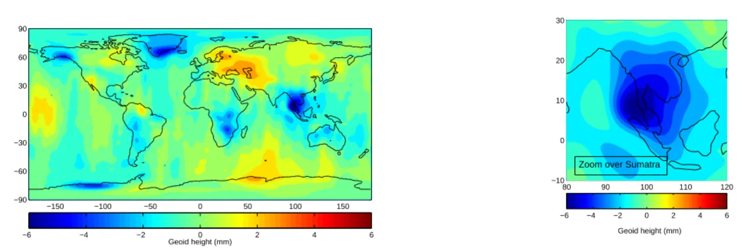
Permanent effect. To confirm the permanent nature of the systematic displacement of the geoid in the zone of Sumatra around the date of the earthquake, we have estimated for each point of the grid the constant term on the period preceding this date and the constant term on the period after the seism, the difference ∆h constituting the permanent effect at the point considered. The result appears on the Fig. 3 and reveals in an obvious way that the geoid dropped overall in the area of Sumatra by approximately 6 mm. The formal uncertainties of the estimated shifts are lower than 0.5 mm over Indenosia, and globally lower than 0.7 mm. That corresponds to the precision given by Wahr et al. (2006) (see section 2), and those offsets present a ratio ”signal/noise” larger than 6. Notice that the shift is more considerable than for the two consecutive grids around the seism date (Fig. 1).
To confirm this effect, we carried out the same calculation for other consecutive time in-tervals, which precede that of the seism and we noted that the Indonesia did not arise, as illustrated by the whole set of graphs of the Fig. 4-A/B/C. For consecutive periods after the seism (May 2005) the difference of the constant terms is also quasi null on Sumatra (Fig. 4-D). That confirms the fact that the drop observed in the Sumatra region is well associated with the date of December 26, 2004.
−150 −100 −50 0 50 100 150 −90 −60 −30 0 30 60 90 Geoid height (mm) −6 −4 −2 0 2 4 6 80 90 100 110 120 −10 0 10 20 30 Geoid height (mm) −6 −4 −2 0 2 4 6
Zoom over Sumatra
Figure 3: Difference of constant terms estimated after and before the Sumatra seism.
−150 −100 −50 0 50 100 150 −90 −60 −30 0 30 60 90 Geoid height (mm) −6 −4 −2 0 2 4 6
(A)[July 2002-July 2004]-[July 2004-Dec. 2004]
−150 −100 −50 0 50 100 150 −90 −60 −30 0 30 60 90 Geoid height (mm) −6 −4 −2 0 2 4 6
(B)[July 2002-Jan. 2004]-[Jan. 2004-Dec. 2004]
−150 −100 −50 0 50 100 150 −90 −60 −30 0 30 60 90 Geoid height (mm) −6 −4 −2 0 2 4 6
(C)[July 2002-Jan. 2003]-[Jan. 2003 -Dec. 2004]
−150 −100 −50 0 50 100 150 −90 −60 −30 0 30 60 90 Geoid height (mm) −6 −4 −2 0 2 4 6
(D) [Jan. 2005-May 2005]-[May 2005-Sep. 2005]
Figure 4: Difference of constant terms estimated over two consecutive time intervals before the seism (A), (B), (C); after the seism (D) : no drop observed in Indonesia.
4
Rotational effect
Influence of an Earthquake on the Earth rotation When mass redistribution occurs inside the Earth, off-diagonal elements of the earth inertia matrix referred to the cartesian terrestrial frame 0xyz c13 = −RMexz dm and c23 = −
R
Meyz dm can change, as well as the
equatorial relative angular momentum h = h1+ ih2. It follows that the Earth wobbles around
the rotation axis in space, and from a terrestrial point of view the rotation axis moves with respect to the crust. For an elastic Earth model, the coordinates of the Celestial Intermediate Pole p = x − iy obey the equation (see e.g. Munk and MacDonald, 1960):
p + i ˙p σC = ks ks− k2 ( c (C − A) + h (C − A)Ω) (6) where Ω is the mean Earth angular velocity, c = c13+ ic23, C the axial inertia moment of the
Earth, A the equatorial one, k2 ≈ 0.3 the Love number of degree 2, ks≈ 0.94 the Secular Love
number, σC the Chandler pulsation (Ω/433 ≈ ksk−ks 2(C − A)/A). In the case of an earthquake,
c can be modeled as a step function. The effect of relative angular momentum h is negligible, because it is not permanent. Then it can be easily shown that the consequence of the polar motion is a sudden offset of the pole, and a modification of the amplitude of the Chandler component according to : ∆p = Ωc Aσc − Ωc Aσc eiσC(t−t0) (7) Mass redistribution is also accompanied by variation of axial inertia moment, c33 and axial
angular momentum h3. In virtue of the angular momentum conservation of the solid Earth
the rotation velocity is changed, equivalently Length of Day LOD0 undergoes the increment
∆LOD given by : ∆LOD LOD0 = c33 C + hr 3 ΩC (8)
Angular momentum associated with seismic displacements is huge (typically 1028 kg m2 s−1,
see Seoane, 2006) during the first 100 µs, but disappears after the seism (typical duration of 10 minutes). The only remaining effect is that of the axial inertia increment.
Changes of the Stokes coefficients of degree 2 and inertia moments of the Earth. The drop of the geoid height over Indonesia provides the changes in the Stokes coefficients C21, S21, C20 caused by the seism. Hence, by the relations (2), (3) and (5) we obtain the
increments in inertia moments c13= ∆I13, c23= ∆I23 and c33= ∆I33.
Variation of geopotential Wo (δW ) before and after the seism is obtained from the
modifi-cation of geoid height.
Indeed let us place on a point P on the geoid before the seism where the potential is Wo.
After the seism, in this same point, the potential becomes Wo+ ∆W . Let us consider a point
P0 being located on the deformed geoid and on the same line of force than P. We have on this
line of force :
WP0 − WP = ~∇W.
−→ PP0
By projection on the outer normal to the geoid ( ~n ), this equation is written : Wo− (Wo+ ∆W ) = dW d~n ∆h = −g∆h that is : ∆W = g∆h (9)
where ∆h is the variation of geoid height and g the field of gravity, which can be considered as constant (g = 9.83 m s−2) in order to evaluate ∆W starting from h. Having obtained
∆W , we shall calculate the corresponding Stokes coefficients ∆C21 and ∆S21. To isolate the
effect of Sumatra, ∆W is restricted to the associated area (the fluctuation ∆W is taken as null everywhere else). Moreover we make the approximation r = Re. The variations of the Stokes
coefficients result from the well-known relations : ∆C20 = Re GMe 5 4π Z Z S ∆W (θ, λ)P20(cos θ) sin θ dθ dλ ∆C21 = Re GMe 5 12π Z Z S
∆W (θ, λ)P21(cos θ) cos λ sin θ dθ dλ
∆S21 = Re GMe 5 12π ZZ S
∆W (θ, λ)P21(cos θ) sin λ sin θ dθ dλ
(10)
These double integrals are computed by trapezoidal method.
Determination of the area affected by the seism. Actually it is a rather delicate task to determine the area which has to be taken in these integrals. The larger is the surface, the more will be integrated fluctuations not linked with Sumatra event, and the influence of the errors will grow. Displacements of the ground surface as observed by GPS (Vigny et al., 2005) suggest to consider circular zone of 30◦ arc radius around the epicenter. On the other hand,
the seismic area S can be deduced from the seismic moment M = µSD where µ is the shear modulus (≈ 75 Gpa) and D is the slip (D = 10 m). The typical value for the seismic moment (for a review see Gross and Chao, 2006), M ≈ 1023 Nm, gives a typical aftershock area surface
of 100 000 km 2 (3o x 3o). This can be considered as the smallest zone disturbed by the seism.
Anyway there is no a priori reason to privilege a given surface. Therefore computations were done for spheric caps centered on the epicenter (latitude 3.5o and longitude 95.5o) of increasing
area, from 3◦ to 180◦ (the whole Earth’s surface).
Effect on polar motion. The effect on the rotation pole follows from equation (7): p(t) = x − iy = Ω(∆I13+ i∆I23)
Aσc
(1 − eiσct) (11)
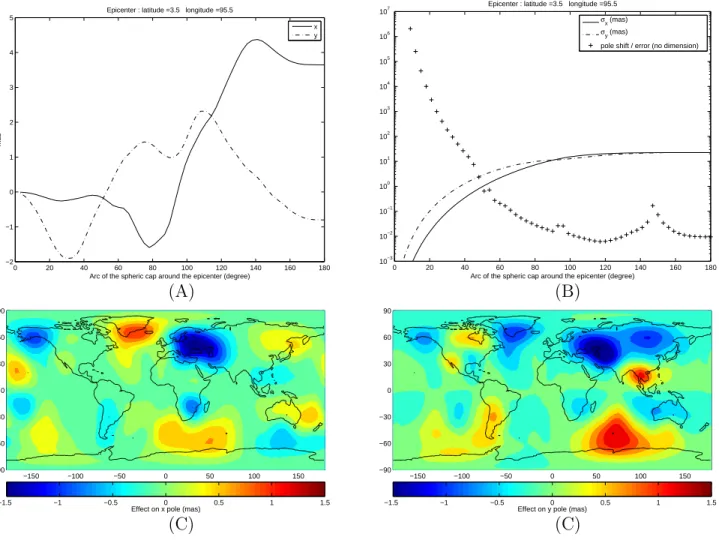
On Fig. 5-A, the x and y components of the polar shift p = Ω(∆I13+ i∆I23)/(Aσc) are
strong dependence on the area. Whereas x remains below 0.3 mas for regional area (below 30o), the y component present a significant increase, and reaches a local minimum of -2 mas for
the arc radius of 30o. We attempted to assess the precision of these results. The uncertainties,
displayed on 5-B, are obtained from the integrals taking absolute value of the function to be integrated and ∆W = gσh ; σh is the “mean error” of the permanent geoid shift, taken equal
to 0.5 mm (see section 3). From radius larger than 40o, the ratio of the pole shift |p| over its
uncertainty drops below 3, and contribution of the ice caps becomes dubious.
To get a better insight of the effective seismic area, we plot on Fig. 5-C/D the contribution on polar motion of each 10o radius spherical cap over the 5o x 5o latitude-longitude grid. Clear
patterns take shape, putting forward the Sumatra effect (on y pole exclusively) and important contributions of Central Asia (-1.5 mas for y), South Indian Ocean/Antarctic (1 mas for y) and Greenland (1 mas for x). The strong variations observed in Central Asia and Indian Ocean cannot be caused by the Sumatra Earthquakes, they have other causes either hydrological or linked with oceanic circulation. Therefore the effective seismic zone cannot be hardly extended beyond 30o. Then, if we favor the 30o spheric cap as the effective seismic area, the “Sumatran
polar shift” as well the corresponding inertia increment and Stokes coefficients admit the values reported in table 1.
∆C21 ∆S21 ∆I13 ∆I23 Polar motion shift (mas)
(kg m2) x y
9.0 10−13 −7.0 10−12 −2.1 1026 1.7 1027 −0.25 ± 0.1 −2 ± 0.5
Table 1: Sumatra pole shift for 30o spheric cap around the epicenter
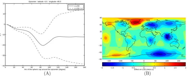
Effect on the length of day. From equation (8) the length of day undergoes a constant variation :
∆LOD LOD0
= ∆I33
C (12)
On Fig. 6-A, the LOD increment is showed as a function of the arc radius of the spheric cap around the epicenter. We notice a continuous decreasing until 80o. The increment becomes
stable from 120o and reach constant value of −13µs. Error are computed in a way similar to
those for polar shfit and are also drawn on Fig. 6-A. We plot on Fig. 6-B the contribution on LOD of each 10o radius spherical cap over the a 5o x 5o latitude-longitude grid covering the
Earth. Strongest fluctuations patterns appears in the same area as for polar motion. However a peculiar feature appears : negative increments in the eastern hemisphere and positive in the western ones.
Then, if we favor the 30o spheric cap as the effective seismic area, the “Sumatran LOD
change” as well the corresponding inertia increment and Stokes coefficient admit the values reported in table 2.
0 20 40 60 80 100 120 140 160 180 −2 −1 0 1 2 3 4 5
Arc of the spheric cap around the epicenter (degree)
mas
Epicenter : latitude =3.5 longitude =95.5
x y (A) 0 20 40 60 80 100 120 140 160 180 10−3 10−2 10−1 100 101 102 103 104 105 106 107
Arc of the spheric cap around the epicenter (degree) Epicenter : latitude =3.5 longitude =95.5
σx (mas)
σy (mas)
pole shift / error (no dimension)
(B) −150 −100 −50 0 50 100 150 −90 −60 −30 0 30 60 90
Effect on x pole (mas)
−1.5 −1 −0.5 0 0.5 1 1.5 (C) −150 −100 −50 0 50 100 150 −90 −60 −30 0 30 60 90
Effect on y pole (mas)
−1.5 −1 −0.5 0 0.5 1 1.5
(C)
Figure 5: Pole shift in function of the spheric cap : x/y pole on increasing spheric caps centered around the epicenter (A) ; uncertainties on pole shift estimates (B); x pole on 10o spheric caps
0 20 40 60 80 100 120 140 160 180 −40 −30 −20 −10 0 10 20
Arc of the spheric cap around the epicenter (degree)
µ
s
Epicenter : latitude =3.5 longitude =95.5
∆ LOD ∆ LOD ±σ (A) −150 −100 −50 0 50 100 150 −90 −60 −30 0 30 60 90
Effect on LOD (micro s)
−2 −1.5 −1 −0.5 0 0.5 1 1.5 2
(B)
Figure 6: LOD increment in function of the spheric cap : over increasing spheric caps centered around the epicenter (A) ; over 10o spheric caps (B)
∆C20 ∆I33 LOD increment
(kg m2) (µs)
2.8 10−11 −4.6 1027 −5.0 ± 1.5
Table 2: Sumatran effect on the length of day
5
Discussion
Thanks to the data of the mission GRACE combined with those of LAGEOS, seismic effect on terrestrial rotation has been estimated independently from a geophysical model. Our re-sults have to be compared to the ones derived by the classical approach, integrating seismic parameters into dislocation models. Such an estimation have been done by Bizouard (2005) (model of Dahlen, 1973) and Gross and Chao (2006). As shown in the table 3, both models give more or less convergent value for polar shift. The amplitude, according to the assimilated seismic parameters, can reach 1-2 mas, typical value that we also obtained for 20-30o spheric
caps around the epicentre. Geophysical models give a prevalent effect for x component (along Greenwich meridian), whereas it is always the opposite for us (see Fig. 5-A). The geopotential approach contradict seismic modeling, which might be too simplistic. Therefore we call into question the modeling of seismic displacements or the observed seismic parameters.
C.Bizouard(2005) Gross and Chao(2006) Param. Sism. Haward CMT −0.7 + i 0.1 mas −0.7 + i 0.5 mas
Param. Sism. Stein (2005) −1.7 + i 0.45 mas
Table 3: Sumatran effect on polar motion from seismic displacement modeling : C. Bizouard (2005) (two sets of seismic parameters) and Gross and Chao (2006).
The effect (≈ 1 mas) is well above the precision of the observations (0.05 mas). However it is not easily separable from other geophysical excitation on this date, that is why nobody could clearly highlight it. In the past the seisms of Chile (1960) and Alaska (1964) would have caused a shift of the pole higher than 10 mas (30 cm), that would have been easily detected by the current techniques.
For the length of the day Chao & Gross (2006) modeled the increment of axial inertia mo-ment and obtained a drop of 2-6 µs confirmed by our result (5 µs). This effect is undetectable in the LOD, because the precision on this parameter is of 20 µs.
These results are founded on hypothesis that the earthquake caused permanent geoid dis-placement. Actually, post-seismic deformation can produce relaxation of the geoid. The exten-sion of GRACE data will allow us to investigate post-seismic evolution. On the other hand, we could better isolate the seismic effect by modeling and removing the hydrologic influence on the gravity field.
This study is a bright demonstration of the richness of the observations of the satellites GRACE supplemented by those of satellites LAGEOS. They made possible to reconstitute the gravity field with a precision and a space resolution such as the global redistributions yesterday invisible have been lately “photographed”. Thus they lead to the possibility of constraining model of seismic displacement, and more generally determine internal mass motion. Besides this pure geophysical interest, they allow us to investigate episodic changes in Earth’s rotation.
AcknowledgmentsThis study started when Sylvain Loyer (Centre National d’Etude Spatiale, CNES) showed us his rough determination of the Sumatran drop in geoid height. We also highly appreciate the help of his co-worker Jean-Michel Lemoine (CNES) for the GRACE data description.
References
[Biancale(2005)] Biancale R., J.M. Lemoine, G. Balmino, S. Bruinsma, F. Perosanz, J.C. Marty, S. Loyer, P. G´gout, Strasbourg (2005), 3 years of geoid variations from GRACE and LA-GEOS data at 10-day intervals over the period from July 29th, 2002 to September 30th, 2005, http://bgi.cnes.fr:8110/geoid-variations/README.html or CD-ROM, CNES/GRGS product.
[Bizouard(2005)] Bizouard, C. (2005), Influence of the Earthquakes on Polar Motion with Em-phasis on the Sumatra Event, published in Actes Les Journ´ees Systmes de R´ef´erence 2005 CBK Warsaw.
[Dahlen(1973)] Dahlen, F.A. (1973), A correction to the excitation of the Chandler woobble by earthquakes. Geophys. J. R. astr. Soc. 32 : pp. 203-217.
[Chao(2006)] Gross, R., Chao B.F (2006), The rotational and gravitational signature of the December 26, 2004 Sumatran earthquake, Surv. Geophys. DO1 10.1007/s10712-006-9008-1.
[Lambeck(1980)] Lambeck, K. (1980), The Earth’s Variable Rotation: Geophysical Causes and Consequences. Cambridge University Press.
[Lemoine(2006)] Lemoine, J.M., 2006, private communication. [Loyer(2006)] Loyer, S., 2006, private communication.
[Mikhailov(2004)] Mikhailov V., Tikhotsky S., Diament M., Panet I., Ballu V. (2004), Can tectonic processes be recovered from new gravity satellite data. Earth and Planetary Science Letters 228, 281-297.
[Mink(1960)] Munk, W.H and MacDonald, G.J.F (1960), The Rotation of the Earth, Cam-bridge University Press.
[Rochester(1974)] Rochester, M.G., and Smylie, D.E. (1974), On Changes in the Trace of the Earth’s Inertia Tensor. J.Geophys. Res. : 89, pp. 1077-1087.
[Seoane(2006)] Seoane L. (2006), Nouveaux aperus sur la rotation terrestre partir de l’observation du champ de gravit´e, Rapport de Stage de Master M2, Observatoire de Paris. [velicogna1(2005)] Velicogna, I., and Wahr, J. (2005), Greenland mass balance from GRACE.
Geophysical Research Letters : Vol. 32.
[velicogna2(2005)] Velicogna, I., Wahr, J., Hanna, E. and Huybrechts, P., (2005), Short term mass variability in Greenland, from GRACE. Geophysical Research Letters: Vol. 32.
[Vigny(2005)] Vigny, C., Simons, W.J.F, Abu, S., Bamphenyu, R., Satirapod, C., Choosakul, N., Subarya, C., Socquet, A., Omar, K., Abidin, H.Z. and Ambrosius, B.A.C. (2005), Insight into the 2004 Sumatra-Andaman Earthquake from GPS Measurements in Southeast Asia. Nature : Vol 436.
[Wahr(2006)] Wahr, J., Swenson, S. et Velicogna, I. (2006), Accuracy of GRACE mass esti-mates. Geophysical Research Letters, Vol. 33.