HAL Id: hal-01677362
https://hal.sorbonne-universite.fr/hal-01677362
Submitted on 8 Jan 2018
HAL is a multi-disciplinary open access archive for the deposit and dissemination of sci-entific research documents, whether they are pub-lished or not. The documents may come from teaching and research institutions in France or abroad, or from public or private research centers.
L’archive ouverte pluridisciplinaire HAL, est destinée au dépôt et à la diffusion de documents scientifiques de niveau recherche, publiés ou non, émanant des établissements d’enseignement et de recherche français ou étrangers, des laboratoires publics ou privés.
Impact of a shallow groundwater table on the global
water cycle in the IPSL land–atmosphere coupled model
Fuxing Wang, Agnès Ducharne, Frédérique Cheruy, Min-Hui Lo, Jean‑yves
Grandpeix
To cite this version:
Fuxing Wang, Agnès Ducharne, Frédérique Cheruy, Min-Hui Lo, Jean‑yves Grandpeix. Impact of a shallow groundwater table on the global water cycle in the IPSL land–atmosphere coupled model. Climate Dynamics, Springer Verlag, In press, �10.1007/s00382-017-3820-9�. �hal-01677362�
Impact of a shallow groundwater table on the global water cycle
in the IPSL land–atmosphere coupled model
Fuxing Wang1 · Agnès Ducharne2 · Frédérique Cheruy1 · Min‑Hui Lo3 · Jean‑Yves Grandpeix1
25°S–60°S) are significantly impacted by the WT, showing a decrease in air temperature (−0.5 K over mid-latitudes and −1 K over tropics) and an increase in precipitation. The latter can be explained by more vigorous updrafts due to an increased meridional temperature gradient between the equator and higher latitudes, which transports more water vapour upward, causing a positive precipitation change in the ascending branch. Over the West African Monsoon and Australian Monsoon regions, the precipitation changes in both intensity (increases) and location (poleward). The more intense convection and the change of the large-scale dynamics are responsible for this change. Transition zones, such as the Mediterranean area and central North America, are also impacted, with strengthened convection resulting from increased ET.
Keywords Groundwater table · Land–atmosphere · Near
surface climate · IPSL-CM · West African Monsoon 1 Introduction
Groundwater systems are dynamic and adjust to many factors (e.g., climate changes, groundwater withdrawal, land use, terrain elevation, slope, etc.). Observations show that water table depths vary at diurnal, seasonal and inter-annual scales (Fan et al. 2007), and recent changes in groundwater storage can be detected across almost the whole globe (Richey et al. 2015). Modelling studies based on climate change projections by General Circu-lation Models (GCMs, e.g., ECHAM4, HadCM3), usu-ally downscaled and bias-corrected, reveal large poten-tial changes of groundwater recharge and related water resources, that can exceed ±30% by the 2050s, but with
Abstract The main objective of the present work is to
study the impacts of water table depth on the near surface climate and the physical mechanisms responsible for these impacts through the analysis of land–atmosphere coupled numerical simulations. The analysis is performed with the LMDZ (standard physics) and ORCHIDEE models, which are the atmosphere-land components of the Institut Pierre Simon Laplace (IPSL) Climate Model. The results of sensitivity experiments with groundwater tables (WT) prescribed at depths of 1 m (WTD1) and 2 m (WTD2) are compared to the results of a reference simulation with free drainage from an unsaturated 2 m soil (REF). The response of the atmosphere to the prescribed WT is mostly concen-trated over land, and the largest differences in precipita-tion and evaporaprecipita-tion are found between REF and WTD1. Saturating the bottom half of the soil in WTD1 induces a systematic increase of soil moisture across the continents. Evapotranspiration (ET) increases over water-limited regimes due to increased soil moisture, but it decreases over energy-limited regimes due to the decrease in down-welling radiation and the increase in cloud cover. The tropi-cal (25°S–25°N) and mid-latitude areas (25°N–60°N and
* Fuxing Wang
fuxing.wang@lmd.jussieu.fr
1 Laboratoire de Météorologie Dynamique, IPSL, CNRS, Sorbonne Universités, UPMC, 75005 Paris, France 2 Sorbonne Universités, UPMC, CNRS, EPHE, UMR 7619
METIS, 4 place Jussieu, 75005 Paris, France
3 Department of Atmospheric Sciences, National Taiwan University, Taipei, Taiwan
uncertain regional patterns (Döll 2009; Taylor et al.
2013; Portmann et al. 2013; Habets et al. 2013).
Conversely, the fluctuations of groundwater levels have potential impacts on the climate due to their influence on soil moisture profiles and ET rates. Many studies have shown that the inclusion of groundwater processes in land surface models improves the simulated water budget over land (e.g. Ducharne et al. 2000; Liang et al. 2003; Xie et al. 2012; Maxwell et al. 2015). However, stud-ies regarding the feedback of groundwater change to the climate are limited. Yuan et al. (2008) show that incor-porating water table dynamics into the regional climate model RegCM3 significantly increases the recycling rate and precipitation efficiency over semiarid regions (local aquifer-atmosphere feedbacks) in the East Asian mon-soon area. Anyah et al. (2008) find that the groundwater table induces an enhanced ET in the more arid western regions of the United States, where soil water is a strong limiting factor of ET. In the more humid regions (where ET is rather limited by surface energy availability), the wetter soil does not generally lead to systematic increases in ET. Jiang et al. (2009) report that the incorporation of vegetation and groundwater dynamics into the Weather Research and Forecasting (WRF) model produces more precipitation in the Central United States, which is related to a positive land–atmosphere feedback mechanism in the summer, also reported over Europe by Campoy et al. (2013). Modelling studies also indicate that groundwater-fed irrigation increases ET by 4% over the continental United States (Ozdogan et al. 2010) and increases down-wind precipitation by 15–30% in the high plains of the United States in July (De Angelis et al. 2010). Similar effects are found in response to anthropogenic groundwa-ter exploitation by Zen et al. (2017) and Zou et al. (2014), at global and at regional scales, respectively.
Most of the above studies/analyses have been carried out at regional scales (e.g., over Asia and the United States). At the global scale, Lo and Famiglietti (2011) analyse the con-tributions of groundwater dynamics to the spatial–temporal variability of precipitation by using the National Center for Atmospheric Research (NCAR) Community Atmosphere Model. The addition of groundwater yields an increase of precipitation in the tropical land regions of the North-ern Hemisphere in the boreal summer (explained by the ‘rich get richer’ mechanism; that is, the Hadley circulation transports more water vapour upward, causing a positive precipitation anomaly in the ascending branch) and in the transitional climatic zones (e.g., Central US, Sahel) where soil moisture and precipitation are strongly coupled (Koster et al. 2004). Krakauer et al. (2013) suggest that adding an aquifer to the Goddard Institute for Space Studies (GISS) ModelE GCM affects the seasonality and inter-annual per-sistence of the soil moisture and climate.
The motivation of the present study is to further inves-tigate the global scale responses of climatic variables and patterns to the groundwater table, through model analysis. We use a state-of-the-art land–atmosphere model, which is part of the full IPSL climate model involved in all the CMIP (Coupled Model Intercomparison Project) phases. Our specific objective is to elucidate the physical mecha-nisms that are responsible for the precipitation changes when a groundwater table is accounted for beneath the land surface over the entire globe. To provide a systematic assessment of the impacts of water table depth (WTD) on near surface climate, the proposed protocol overlooks the space and time variations of the WTD, which is set to be constant at different depths. The numerical experiment and the methodology for the analysis are described in Sect. 2. The impacts of the water table depth on global scale evapo-ration, precipitation and land–atmosphere coupling are dis-cussed in Sect. 3. Conclusions are drawn in Sect. 4. 2 Numerical design
2.1 The LMDZOR model
The land–atmosphere coupled simulations are performed with the LMDZ-ORCHIDEE model, which is a compo-nent of the IPSL climate model. It couples the ORCHI-DEE land surface model (De Rosnay et al. 2002; Krinner et al. 2005) and the LMDZ5A atmospheric model (Hourdin et al. 2006), which includes a robust version of the physics code, known as the standard physics and also used in the IPSL-CM5A climate model (Dufresne et al. 2013). Radia-tion follows the scheme of Fouquart and Bonnel (1980) for the solar contributions and of Morcrette et al. (1986) for the infrared contributions. In the planetary boundary layer, the turbulent transport is parameterized via a vertical diffusion approach (Laval et al. 1981), and the Louis (1979) method is applied to describe the surface boundary layer. Conden-sation is parameterized separately for convective and non-convective clouds. For non-non-convective clouds, the cloud cover and cloud water content are deduced from the large-scale total water (vapor + condensed) and moisture at sat-uration (Bony and Emanuel 2001). In convective regions, the parameterization of clouds is coupled to the convective scheme of Emanuel (1991), with condensation and rainfall as the fundamental outputs. The resulting precipitation is characterized as convective precipitation.
In this study, ORCHIDEE includes a dynamic phenol-ogy (simulated by the STOMATE module), through which the leaf area index (LAI) responds to the environmental conditions (Krinner et al. 2005). The vegetation carbon pools (including leaf mass and thus LAI) are prognostically calculated as a function of a dynamic carbon allocation,
fed by photosynthesis, which is positively linked to tran-spiration, and evolves with the surface water and energy budgets. The latter are calculated at the grid cell scale with classical soil-vegetation-atmosphere-transfer formulations, through which the evapotranspiration is partitioned into four parallel fluxes, namely transpiration, bare soil evapora-tion, interception loss, and snow sublimation.
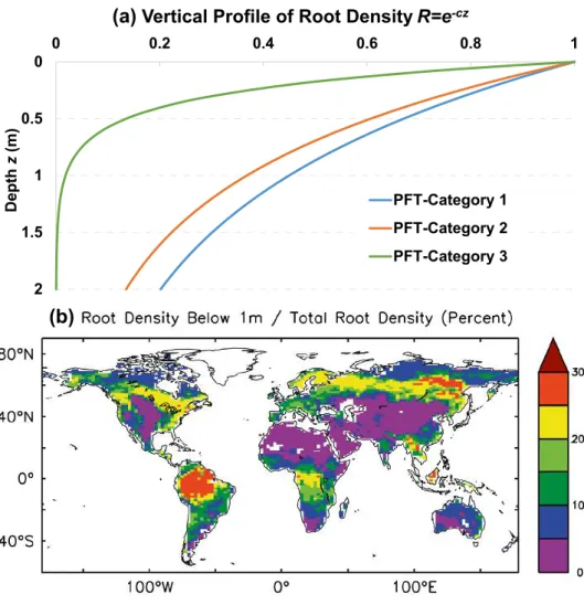
In each grid cell, the vegetation heterogeneity is described using fractions of different plant functional types (PFTs), deduced from high resolution land cover maps. In the present study, we use the maps used for the IPSL-CM5 simulations (Dufresne et al. 2013). In each PFT but the bare soil one, all the vegetation properties depend on the PFT through look-up tables. This is the case of the root density, which decreases exponentially with depth, with a decay factor depending on the PFT (Fig. 1a). The resulting root profiles are constant over time, and expand over the full soil depth for all the PFTs, although the forest PFTs have more deep roots than the crops and grasses (Fig. 1b). Another important PFT property is the fraction that is effectively covered by foliage, which increases exponentially with the LAI owing to an extinction coefficient of 0.5 (Krinner et al.
2005). The complementary fraction is assumed to be bare of vegetation, and does not contribute to interception loss nor transpiration but only to bare soil evaporation.
The latter two fluxes depend on soil moisture and their calculation is coupled to the soil hydrology processes. As detailed in Campoy et al. (2013), the unsaturated water flow is described at each land point by the one-dimensional Richards equation, transformed to use volumetric water content θ (in m3/m3) as a state variable:
in this equation, z is the vertical coordinate (m), counted positively downward; t is time (s); K is the unsaturated hydraulic conductivity (m/s); and D is the soil water dif-fusivity (m2/s), which links θ to the matric potential.
These two parameters are described based on the Mualem (1976)—Van Genuchten (1980) model, with parameters taken from Carsell and Parrish (1988). They depend on the dominant soil texture of each grid cell, defined here from the soil texture map of Reynolds et al. (2000). The lateral (1) 𝜕𝜃 𝜕t = − 𝜕 𝜕z [ D(𝜃)𝜕𝜃(z, t) 𝜕z − K(𝜃) ] − s(z, t),
Fig. 1 The vertical profile of
root density over 2 m depth over three different plant func-tion types a: category 1 (blue,
c = 0.8) corresponds to tropical broad-leaved evergreen, tropi-cal broad-leaved rain-green, temperate broad-leaved ever-green, temperate broad-leaved summer-green, and boreal needleleaf summer-green, category 2 (orange, c = 1) corre-sponds to temperate needleleaf evergreen, boreal needleleaf evergreen, and boreal broad-leaved summer-green, category 3 (green, c = 4) corresponds to C3/C4 grass/agriculture; and the cumulated root density below 1 m compared to total root density (%, b) 0 0.2 0.4 0.6 0.8 1 0 0.5 1 1.5 2 Depth z (m)
(a)
Vertical Profile of Root Density R=e-czPFT-Category 1 PFT-Category 2 PFT-Category 3
fluxes between adjacent grid cells are neglected, and the internal vertical water fluxes are only driven by a sink term, s(z,t) (in m3/m3/s), representing the extraction of water by
roots to fulfil transpiration, and by water fluxes at the top and bottom soil boundaries: infiltration and bare soil evapo-ration at the top; gravitational drainage at the bottom. The soil depth is 2 m with 22 layers, including 22 calculation nodes (the 16 deepest nodes are regularly spaced at every 12.5 cm, while the top 6 are denser).
At the soil bottom, gravitational drainage equals the hydraulic conductivity K(θ) of the bottom node. At the soil surface, the water infiltration rate is limited by the hydrau-lic conductivity of the surface layers, which defines a Hor-tonian surface runoff (d’Orgeval et al. 2008). The bare soil evaporation originates from the bare soil fraction of the grid cell, and proceeds at a potential rate, unless soil water becomes limiting. The transpiration originates from the grid cell fraction that is effectively covered by foliage, for the part with no intercepted water. It is calculated from the potential evaporation limited by a stress function which depends on the soil moisture profile convoluted to the root density profile (de Rosnay et al. 2002).
The solar forcing, greenhouse gases, aerosols, land-use, sea surface temperatures (SST), and sea-ice exhibit inter-annual variability, following the AMIP5 protocol (the fifth phase of the Atmospheric Model Intercomparison Project, Taylor et al. 2012). The model resolution used for this study is 144 (longitude) × 142 (latitude) with 39 vertical levels, and the integration time step is 30-min. The LMDZ-ORCHIDEE model demonstrates good skills in simulating the hydrological cycle at global scales (e.g., Hourdin et al.
2006; Dufresne et al. 2013; Brands et al. 2013).
2.2 The sensitivity experiment
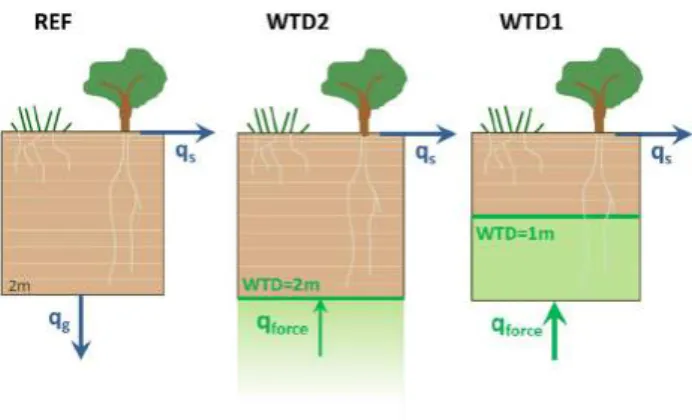
In the control simulation (REF), ORCHIDEE is run with a 2-m soil, discretized along 22 calculation nodes, with free gravitational drainage at the soil bottom. The sensitivity tests are designed by forcing a globally uniform water table at different depths, 1 and 2 m, corresponding to the sim-ulations WTD1 and WTD2, respectively (Fig. 2). To this end, all of the calculation nodes at or below the prescribed WTD are forced to remain saturated, which corresponds to replacing the gravitational drainage with an upward water flux, offsetting the soil moisture depletion by ET (Campoy et al. 2013). In practice, this upward forcing flux (qforce in
Fig. 2) is defined at each time step as the amount of water required to bring the required nodes to saturation after a normal integration of the Richards equation. The latter integration, however, uses an impermeable bottom to pre-vent massive leaching of the saturated layers by continuity if gravitational drainage was maintained.
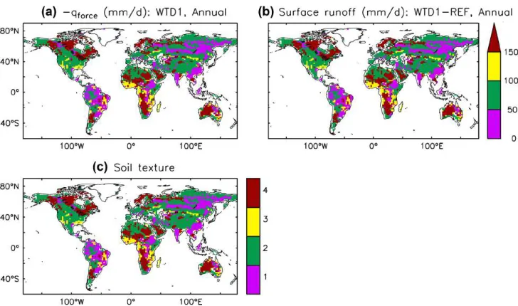
Figure 3a–c shows that very high qforce is needed in
sandy soils, which combine high saturated hydraulic con-ductivity and low matric potential, and therefore easily release water for transpiration. In contrast, the lowest qforce
are found in clay soils, with low saturated hydraulic con-ductivity and high matric potential. This qforce corresponds
to an addition of water to the climate system, which modi-fies the global water balance. This protocol is very similar to the ones where soil moisture or the related water stress on ET is forced, as pioneered by Shukla and Mintz (1982) to assess the influence of the land evaporation rate on the simulated water cycle, and further developed to decipher how the land surface state contributes to the climate vari-ability (GLACE project, Koster et al. 2006) and climate change trajectories (GLACE-CMIP, Seneviratne et al.
2013). In comparison to these pieces of work, qforce allows
us to quantify how we violate the water balance (Fig. 3a), and to better analyze the consequences. We find that qforce
mostly transfers to surface runoff, which increases a lot in simulation WTD1 to evacuate the forced water input that does not lead to increased soil moisture or ET (Fig. 3b). This surface runoff increase has no impact on the simu-lated climate, since the ocean’s water budget is overlooked in AMIP simulations. Note the water budget is perfectly closed when qforce is included in the calculation.
Another issue with the proposed experiment design is that we force a uniform water table depth regardless of rooting depth variations, so the direct tapping from the roots below the water table might strongly shape our results. This assumption can be rejected at first order for the LMDZOR model since most regions have a small percent-age of deep roots (<10% below 1 m, Fig. 1b). Logically, the smallest values correspond to arid areas with sparse veg-etation, and the highest ones are found in densely forested
Fig. 2 Schematic of the main soil water fluxes in the control
simu-lation (REF) and in the forced water depth simusimu-lations (WTD2 and WTD1). The unsaturated and saturated zones are depicted in brown and green, respectively, and the represented water fluxes are the sur-face runoff (qs), drainage (qg), and upward forcing flux (qforce)
areas (Amazon, Indonesia, Eastern Russia), but they remain under 30%, and the cumulated root density is much smaller below than above 1 m (>70%).
For initialization, we start with equilibrium soil moisture maps obtained from preliminary warm-up simulations with the above versions of ORCHIDEE in off-line mode (using meteorological forcing from Sheffield et al. 2006). The LMDZOR model is then spun up for 10 years with a clima-tological SST. The historical simulations follow with inter-annually varying SSTs from 1979 to 2005. We checked that the total soil moisture shows a negligible trend over the last 8 years of the spin-up in at least 98% of the land points according to at least one of two trend criteria: (C1) the linear trend of the total soil moisture content over the evaluation period is less than 1% of the initial moisture; or (C2) the Mann–Kendall trend test (with Sen’s method fol-lowing Burkey 2006) is not significant (p value <0.01 with null hypothesis of no trend).
We carried out each simulations of the paired experi-ment (REF vs WTD1 or WTD2) over 27 years after spin-up, which is considered to be enough to statistically detect mean changes in front of the inter-annual variabil-ity. To this end, we used the Student test to assess if the
simulations have different 27-year means at the significance level of 5%. We also used the Wilcoxon signed-ranked test, which is non-parametric test, to confirm the results (not shown). Many recent studies still use this approach (e.g., Forster 2016; Lin 2016) despite the development of ensem-ble methods.
3 Results and discussions
3.1 Inter‑comparison of globally averaged near‑surface variables
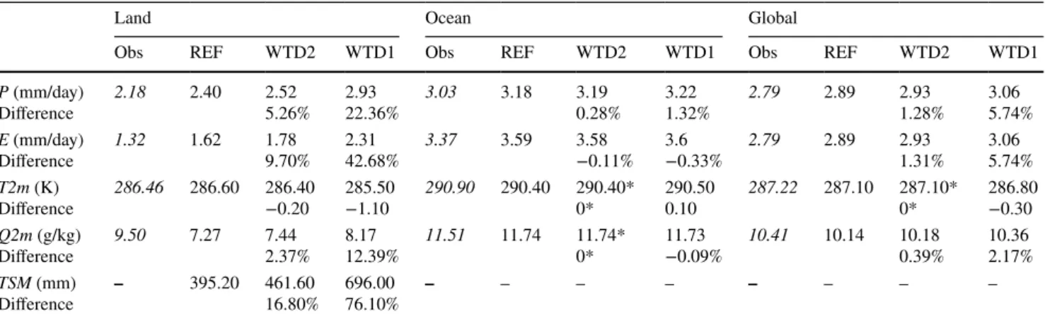
The evaporation (E), precipitation (P), near surface air temperature and humidity (T2M and Q2M) are compared in Table 1 for all simulations (REF, WTD1, WTD2) along with the reference observations/reanalysis data (Rodell et al. 2015; Kalnay et al. 1996) as the averages over land, ocean and globally. For both WTDs, the impacts on the near-surface meteorology are larger over land than over the oceans. This is reasonable because WTs are only pre-scribed over land, and sea surface temperatures are forced in all simulations, as discussed by Krakauer et al. (2016)
Fig. 3 The annual mean forcing flux (qforce, times by −1 to get
posi-tive values, in mm/d) in WTD1 (a), the annual mean difference of surface runoff (in mm/d) between WTD1 and REF (b), and the soil texture map of the two simulations, clustered in four categories (c): category 1 (magenta) corresponds to Silt Loam, Clay Loam, Sandy
Clay, Silty Clay, and Clay of USDA soil textures; category 2 (green) corresponds to Silt, Loam, Silty Clay Loam of USDA soil textures; category 3 (yellow) corresponds to Sandy Clay Loam of USDA soil texture; category 4 (red) corresponds to Sand, Loamy Sand, and Sandy Loam of USDA soil textures
regarding the effect of irrigation on the climate. The pre-scribed saturation at the soil bottom leads to wetter soil in WTD1 and WTD2 than in REF, which induces an increase of E by 10–40%. As a result, the land surface is cooled by about −0.2 to −1.1 K, and precipitation increases by 5–20% in the two simulations with forced WTD. The changes of E, P, Q2M and T2M are monotonous with the decrease of WTD, and the differences between WTD1 and REF are much larger than those between WTD2 and REF. Therefore, we focus hereafter on the comparison between REF and WTD1 to better detect the impact of the WT on the near-surface climate.
3.2 Spatial distributions of near‑surface variable variations over the globe
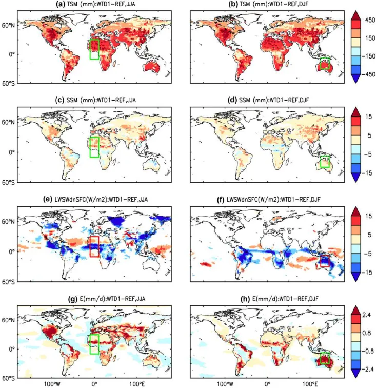
The following analysis is supported by seasonal maps of the differences in the near-surface variables between REF and WTD1 (Figs. 4, 5, 6), complemented by equivalent maps for REF (Fig. S1) and WTD1 (Fig. S2). Note that the difference maps only show colors in grid points where WTD1-REF is statistically significant (with a Student test at the 5% significance level).
The total soil moisture (TSM, over the 2 metres of soil) displays a very widespread increase in WTD1 (Fig. 4a, b). The first order effect comes from imposing saturation across the lowest metre of soil, so the increase is larger in dry areas, where the forced saturation has a larger relative impact. We preferred to focus on the surface soil moisture (SSM, over the top 10 cm), which interacts more directly with the rest of the water cycle. The SSM increases signifi-cantly over most regions between REF and WTD1, in both June–July–August (JJA) and December–January–February (DJF), owing to the capillary rise from the 1 m deep WT (Fig. 4c, d).
Evapotranspiration (ET) is key to the soil moisture— climate interactions and we expect most of the inferred impacts of soil moisture on the climate to be caused by its control on the ET in soil-moisture-limited regimes (Seneviratne et al. 2010). The variability of E over land is controlled by the availability of surface energy (total downwelling solar and thermal radiation fluxes) and the availability of surface soil moisture (e.g., Boé and Ter-ray 2008). Indeed, the soil moisture increase in WTD1 induces a higher E in WTD1, mainly over arid and semi-arid regions, because of reduced water stress (Fig. 4g, h). In contrast, E decreases over tropical regions, owing to the decrease of downwelling radiation at the surface (Fig. 4e, f), which is related with an increase in cloud cover (not shown), as previously shown by Schär et al. (1999). Quan-titatively, most ET changes can be attributed to the tran-spiration (Fig. 5a, b), which increases where both the TSM increase and the total root density is large (Fig. 1). However, most areas with high root density, corresponding to dense deep roots, show weak or negative transpiration change, for two reasons: they are already very wet in the REF simu-lation, and they undergo a decrease of downwelling radia-tion. Eventually, the areas with the largest proportion of deep roots are not the ones with the largest changes of ET or transpiration, which confirms that the direct tapping of the water table by deep roots does not strongly shape the simulation results. The patterns of LAI changes (Fig. 5c, d) closely match those of the transpiration changes, owing to the coupling between the transpiration and photosynthesis. The bare soil evaporation changes (Fig. 5e, f) closely fol-low the SSM variations: bare soil evaporation increases in arid areas, owing to enhanced capillary rise from the 1 m WT, while it decreases where the transpiration increases a lot. The main reason is the increase of LAI, which together increases the potential transpiration and related root water
Table 1 The precipitation (P), evaporation (E), T2m, Q2m and total soil moisture (TSM) in REF, WTD1 and WTD2
The observed latent heat flux and precipitation are from Rodell et al. (2015). The T2m and Q2m are from NCEP reanalysis (1981–2010) (Kalnay et al. 1996). The italic values correspond to observations or reanalyses. The values indicated with * for WTD1 and WTD2 mean the difference from REF is statistically NOT significant (t test, p < 0.05)
Land Ocean Global
Obs REF WTD2 WTD1 Obs REF WTD2 WTD1 Obs REF WTD2 WTD1
P (mm/day) Difference 2.18 2.40 2.525.26% 2.9322.36% 3.03 3.18 3.190.28% 3.221.32% 2.79 2.89 2.931.28% 3.065.74% E (mm/day) Difference 1.32 1.62 1.789.70% 2.3142.68% 3.37 3.59 3.58−0.11% 3.6−0.33% 2.79 2.89 2.931.31% 3.065.74% T2m (K) Difference 286.46 286.60 286.40−0.20 285.50−1.10 290.90 290.40 290.40*0* 290.500.10 287.22 287.10 287.10*0* 286.80−0.30 Q2m (g/kg) Difference 9.50 7.27 7.442.37% 8.1712.39% 11.51 11.74 11.74*0* 11.73−0.09% 10.41 10.14 10.180.39% 10.362.17% TSM (mm) Difference – 395.20 461.6016.80% 696.0076.10% – – – – – – – –
uptake, but also reduces the bare soil fraction from which bare soil evaporation originates.
Because of the cooling effect of E, the 2-m air temper-ature (TAS) and sensible heat flux (not shown) decrease over most regions, but there is a small increase of TAS over the ITCZ in Africa in DJF (Fig. 6a, b). The forcing
of the WT also affects the near-surface specific humid-ity (HUSS, Fig. 5g, h). The variation patterns for HUSS and E are the same in most regions, except in very arid zones (Sahara Desert, Saudi Arabia, Iran), which exhibit the largest HUSS increases while the increase of E is weak. This weak increase comes from the fact that, in
Fig. 4 The difference between REF and WTD1 on average over JJA
(left) and DJF (right) for the total soil moisture (TSM), top 10 cm soil moisture (SSM), downward total radiation at surface (LWSWdnSFC), and evaporation (E). All averages are performed over 27 years (1979–
2005), and the statistical significance of the mean differences is tested at each point with a Student test (p = 0.05). The areas with insignifi-cant changes are left blank
these areas of sparse vegetation, the total ET is largely dominated by bare soil evaporation (Fig. 5a, b, e, f), which benefits from the 1 m WT through capillary rise only, while transpiration can extract water from the entire soil depth through the root profile. The small evapora-tion increase may lead to a strong increase of specific
humidity because the very dry atmosphere in REF over deserts is not prone to convection because of the high surface pressure and remains far from condensation conditions (Fig. S2g, h). This seems consistent with the increase of E being larger than that of P (shown by the reduced P–E).
Fig. 5 Same as Fig. 4 but for transpiration, mean LAI (weighted mean over the vegetation PFTs, excluding the bare soil PFT), bare soil evapora-tion and specific humidity at surface (HUSS)
The change of P from REF to WTD1 occurs mostly over land and mostly in the summer hemisphere (Fig. 6c, d). The most significant variations are found over the Inter-Tropical Convergence Zone (ITCZ), the United States (in JJA), Spain (JJA), and northern Australia (in DJF). Unlike the variations of E (increases over arid regions, decreases over humid regions, Fig. 4g, h), P increases over both arid
and humid regions. Over dry regions (e.g., the western US in JJA, Spain in JJA, northern China in JJA, northern Australian in DJF, etc.), P is quite small in the REF sim-ulation, and it is greatly increased in WTD1 (Figs. 6c, d, S1k, l, S2k,l). The moisture convergence P–E significantly increases over the ITCZ in WTD1 (Fig. 6e, f). In contrast, over the mid-latitudes, the increase in P is often smaller
Fig. 6 Same as Fig. 4 but for 2-m air temperature (TAS), precipitation (P), the moisture flux convergence (P–E), and the convective precipitation (PRC)
than that of E, corresponding to a decrease of P–E, which extends over the coastal oceans. Over the ocean, the P and P–E anomalies are mainly significant over the tropics (e.g., a significant decrease in P over the Indian Ocean in DJF and over the Pacific in both seasons, Fig. 6c, d) and can be explained by changes of atmospheric circulation rather than by local E changes.
We performed the same analysis for the differences between WTD2 and REF (Figs. S3–S5). The change pat-terns are very similar to the ones described above between REF and WTD1, but areas with statistically significant dif-ferences are much smaller, as the magnitude of the corre-sponding differences, in agreement with Sect. 3.1. These weak significant differences in the average maps between WTD2 and REF support that the larger significant differ-ences found between WTD1 and REF are not a statistical accident.
3.3 Impact of WTD on tropical precipitation
To understand the physical mechanisms of the P variations over the tropics, the Hadley and Ferrel circulations are
studied. The zonal mean meridional stream function (ΨM)
is widely used to describe the mean meridional circulation of the atmosphere (e.g., Gastineau et al. 2008; Levine and Schneider 2011). It is given by,
where v is the meridional wind (m/s), a is the radius of the earth (m), p is the air pressure (Pa) and g is the acceleration of gravity (m/s2).
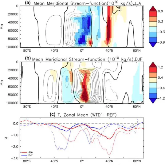
In Fig. 7, the stream-function (global zonal mean) cor-responding to a clockwise circulation is positive (North-ern Hemisphere, DJF), whereas the stream-function cor-responding to a counter-clockwise circulation is negative (Southern Hemisphere, JJA). From REF to WTD1, we find a negative change of the mean meridional stream-function in JJA (over 0–10°N, ascending branch, Fig. 7) and a posi-tive change in DJF (over 5°S–10°N, ascending branch), meaning a strengthened Hadley circulation that has been shifted poleward (northward in JJA and southward in DJF) (2) ΨM= 2𝜋a cos 𝜙 g p ∫ 0 vdp,
Fig. 7 a, b The mean
meridi-onal (both land and ocean) stream-function (1010 kg/s) for JJA and DJF over 1979–2005. The difference between REF and WTD1 is displayed in
colour for the statistically
significant values with p = 0.05, while the values for REF appear as contours (with solid/dashed
lines for positive/negative
values). c The zonal mean of the air temperature integrated from the surface to 800 hPa for WTD1-REF over land + ocean (thick line) and over land (thin
line) in JJA (red) and DJF (blue)
averaged across 1979–2005 [statistically significant (at
p = 0.05) values in solid line and
insignificant values in dashed
in WTD1. The more intense Hadley circulation corre-sponds to a positive precipitation change in the ascending branch (0–15°N in JJA, and 0–15°S in DJF). More specifi-cally, we get a higher moisture convergence over the ITCZ (excluding the Pacific, possibly because this ocean is too large to be significantly affected by changes in ET over land). This is fed by a large zone of decreased convergence (Fig. 6e, f), mostly where there was divergence in REF, which is consistent with the moisture fluxes associated with the meridional Hadley circulation.
Many GCM studies indicate that the Hadley circulation strength is closely related to the meridional temperature gradients (ΔH) between the tropics and mid-latitudes (e.g.,
Levine and Schneider 2011; Seo et al. 2014). The zonal means in Fig. 7c show that the changes in the boundary layer air temperatures (integrated from surface to 800 hPa) from REF to WTD1 are different over the tropics and mid-latitudes. Around the equator, where the temperature is at a maximum in REF, the T decreases by −0.5 K over the globe (−1.0 K over land) in both JJA and DJF. The decrease of T in the boundary layer is larger in the subtropics and mid-latitudes (around −1 K over the globe and −2.5 K over land) than over equator for both JJA and DJF, which leads to a stronger temperature gradient between the equator and mid-latitudes (up to 40°N). This gradient increase is statis-tically significant over both the land and oceans, although less so over the oceans because of the forced SST.
3.4 Impact of WTD on the West African and Australian Monsoons
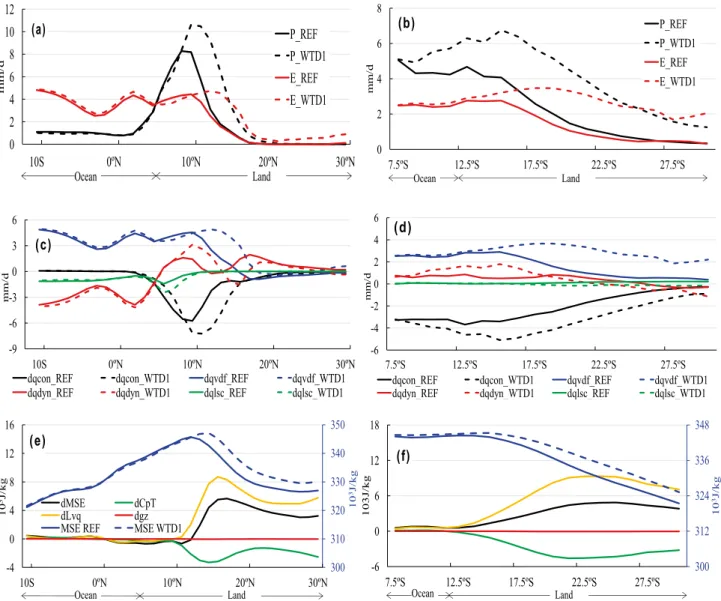
Monsoon systems are linked to the meridional Hadley circulation, although they are strongly altered by smaller scale land/sea contrasts. Over the West African Monsoon (WAM) region, the monsoon flux is below 800 hPa, and it ends between 15°N and 20°N. The location of the maxi-mum precipitation moves from approximately 8°N (REF) to 10°N (WTD1, Fig. 8a).
In July, the monsoon flux is well established and quasi-steady. Hence, the air humidity can be assumed to be constant:
where q is the monthly mean water content of the monsoon flux at a given latitude integrated between the surface and 800 hPa and between 10°W and 10°E; and the indices ‘DYN’, ‘CON’, ‘VDF’, and ‘LSC’ represent the air humid-ity tendencies due to large-scale circulation, convection, boundary layer processes (vertical diffusion of moisture) and large scale condensation, respectively. The moisture flux decomposition in REF and WTD1 for WAM is plotted
(3) 𝜕q 𝜕t | | | |DYN + 𝜕q 𝜕t | | | |CON + 𝜕q 𝜕t | | | |VDF + 𝜕q 𝜕t | | | |LSC ≈ 0,
in Fig. 8c in order to understand the variations of the mois-ture sources/sinks due to the groundwater table. The increased 𝜕q
𝜕t
| |
|DYN (mostly related to changes of the Hadley
circulation) is mainly responsible for the intensified precip-itation between 7°N and 20°N. Between 10°N and 20°N, the increased 𝜕q
𝜕t
| |
|VDF (higher ET from the land surface to the
atmosphere) induces a stronger convection (represented by
𝜕q 𝜕t
| |
|CON) in WTD1, leading to a higher precipitation.
The monsoonal precipitation is also closely linked with the moist static energy (MSE) because the transformation of enthalpy and latent energy available in the lower tropo-sphere into geopotential energy in the upper levels is the main signal of convection (Gaetani et al. 2017). The MSE is defined as,
where gz is the geopotential energy (J/kg), g is the gravi-tational acceleration (m/s2), z is the geopotential height
(m), CpT is the enthalpy (J/kg), Cp is the specific heat of dry air at constant pressure (J/kg·K), T is the temperature (K), Lvq is the latent energy associated with evaporation
and condensation of water (J/kg), Lv is the latent heat of evaporation (J/kg), and q is the specific humidity (kg/kg). Figure 8e shows that the MSE is reinforced over West Africa (10°N–30°N). Among the three components, the latent energy is the main contributor to the MTE difference between REF and WTD1 because of the increased humid-ity in WTD1. The enthalpy becomes lower in WTD1 com-pared to REF because of the decreased temperature. The change in geopotential is small. At local scales, the larger MSE leads to increased convection, favouring larger rain-fall (Zheng and Eltahir 1998; Steiner et al. 2009). This is consistent with the results of Gaetani et al. (2017), who compared the response of the WAM to global warming in several CMIP5 models. They found that the response of IPSL-CM5A, with the same LMDZ5A physics as used in the current study, is dominated by its sensitivity to radia-tive forcing (stronger CO2), leading to an enhanced P over Sahel because of the instability caused by enhanced ET.
The above mechanisms work for the Australian mon-soon (AM) as well. Over the AM region (Fig. 8, right), the maximum precipitation moves further south (from approxi-mately 13°S in REF to 16°S in WTD1). Over 12°S–16°S, the large-scale dynamics (𝜕q
𝜕t
| |
|DYN increases in WTD1) play
a key role in the precipitation change. Over 18°S–30°S (central Australia), the increase in the precipitation in WTD1 is mainly related to the increase in the evaporation (higher 𝜕q
𝜕t
| |
|VDF for WTD1), which leads to higher MSE and
stronger convection (Fig. 8, right). This positive evapotran-spiration-precipitation feedback corresponds to the same
(4) MSE = gz + CpT + Lvq,
mechanism of local moisture recycling involved in the mid-latitudes ‘hot spots’ (as analysed below). The Indian Mon-soon also displays a poleward shift of the monMon-soonal rain belt in Fig. 6c but is not discussed here because the Indian Monsoon is not well represented in REF.
3.5 Impact of WTD on land–atmosphere coupling
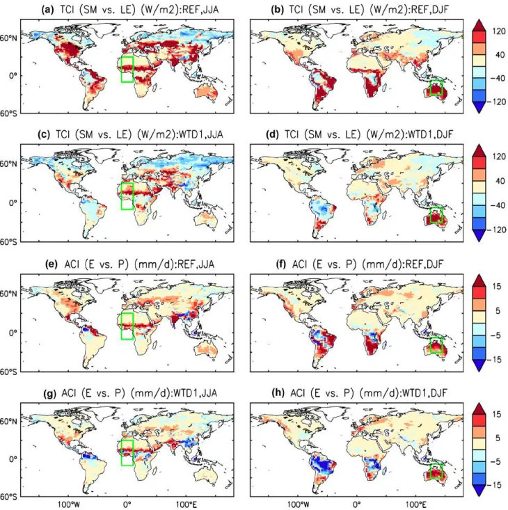
There are various land–atmosphere feedbacks, and we focus on the soil moisture-ET and ET-precipitation couplings. The soil moisture-ET coupling strength is quantified here by the terrestrial coupling index (TCI) of Dirmeyer (2011).
It is based on the correlation of the latent heat flux (LE) and SSM, multiplied by the variance of LE to indicate where the variations of SSM may induce non negligible variations of LE: a positive TCI indicates that the soil moisture sup-ply is the principal control on latent heat flux and a nega-tive TCI indicates that the energy is the limiting factor. The calculation is adapted to monthly data following Dirmeyer et al. (2013) and Cheruy et al. (2014), using 27 monthly mean values for the period 1979–2005. The seasonal val-ues over JJA and DJF are the averages of the corresponding monthly values. In REF, the TCI is strongly positive over areas of transitional soil moisture, including most semi-arid 30ºN 20ºN 10ºN 0ºN 10S 0 2 4 6 8 10 12 d/ m m P_REF P_WTD1 E_REF E_WTD1 Ocean Land (a) 7.5ºS 12.5ºS 17.5ºS 22.5ºS 27.5ºS 0 2 4 6 8 d/ m m P_REF P_WTD1 E_REF E_WTD1 (b) Ocean Land 30ºN 20ºN 10ºN 0ºN 10S -9 -6 -3 0 3 6 d/ m m
dqcon_REF dqcon_WTD1 dqvdf_REF dqvdf_WTD1 dqdyn_REF dqdyn_WTD1 dqlsc_REF dqlsc_WTD1
(c) 7.5ºS 12.5ºS 17.5ºS 22.5ºS 27.5ºS -6 -4 -2 0 2 4 6 d/ m m
dqcon_REF dqcon_WTD1 dqvdf_REF dqvdf_WTD1 dqdyn_REF dqdyn_WTD1 dqlsc_REF dqlsc_WTD1
(d) 300 310 320 330 340 350 30ºN 20ºN 10ºN 0ºN 10S -4 0 4 8 12 16 10 3J/kg 10 3J/kg dMSE dCpT dLvq dgz MSE REF MSE WTD1
Ocean Land (e) 300 312 324 336 348 7.5ºS 12.5ºS 17.5ºS 22.5ºS 27.5ºS -6 0 6 12 18 10 3J/kg g k/ J 3 0 1 Ocean Land (f)
Fig. 8 Comparison of REF (solid line) and WTD1 (dashed line) over
the WAM and AM regions: a, b the precipitation (P, black) and evap-oration (E, red); c, d the four tendencies of the monsoon flux water content due to convection (𝜕q
𝜕t
| |
|CON, black), vertical diffusion in the
boundary layer (𝜕q
𝜕t
| |
|VDF, blue), large scale circulation (
𝜕q
𝜕t
| |
|DYN, red),
and large scale condensation (𝜕q
𝜕t
| |
|LSC, green); e, f the moist static
energy (MSE) for REF (solid blue, axis on right) and WTD1 (dashed
blue, axis on right), the change of MSE (dMSE, black), enthalpy
(dCpT, green), latent energy (dLvq, yellow), and geopotential energy
(dgz, red) integrated from the surface to 800 hPa. All values are aver-aged over 1979–2005 and over 10°W–10°E in WAM in July and over 125°E–145°E in DJF for the AM. The corresponding boxes are
regions, meaning that the soil moisture is the dominant fac-tor that controls the variations of E (Fig. 9a, b). In contrast, E is mainly limited by the available energy at the surface over the regions where TCI is negative (humid regions). The patterns of positive TCIs in REF are strikingly simi-lar to the differences in the ET between WTD1 and REF (Fig. 4g, h), which means that the WTD has an impact on E where there is a strong SSM-E coupling. The coverage of the positive TCI decreases and the coverage of negative
TCI increases in WTD1 (Fig. 9c, d), showing a weakening of the soil moisture-ET coupling strength (Fig. 10a, b). The reason for this is that SSM does not vary much in WTD1, so its covariance with E is smaller than in REF and is not offset by the small variance of the denominator.
Over the mid-latitudes, the most significant impacts of the WT (or soil moisture) on precipitation are positive (P increases) and found over the transition zones where the land–atmosphere coupling is strong (Koster et al. 2004),
Fig. 9 The terrestrial coupling index (TCI, W/m2, a–d) of Dirmeyer et al. (2013), and the atmosphere coupling index (ACI, mm/d, e–h) for REF (first and third row) and WTD1 (second and fourth row) over JJA (left) and DJF (right)
including the central US, Spain, and northern China (Fig. 6c, d). The precipitation variations over the mid-lat-itudes mainly come from increases of convective precipi-tation (Fig. 6g, h). The patterns of increased precipitation
in WTD1 are very consistent with the ones of increased E, which reveals a strong positive ET-precipitation feed-back, despite the decrease in TCI from REF to WTD1 (Figs. 9a–d, 10a, b). Several recent studies also indicate
Fig. 10 The difference between REF and WTD1 for terrestrial
cou-pling index (TCI a, b), atmosphere coucou-pling index (ACI c, d), lift-ing condensation level height (e, f), as well as the correlation between
latent heat flux (LE) and surface specific humidity (HUSS g, h) over JJA (left) and DJF (right)
that this positive land–atmosphere feedback (correspond-ing to a local recycl(correspond-ing of E into precipitation) is the main mechanism responsible for the summer precipitation changes over the central US due to groundwater influence (Lo and Famiglietti 2011; Anyah et al. 2008) and soil mois-ture change (Koster et al. 2004; Ducharne and Laval 2000; Milly and Dunne 1994).
This analysis is confirmed by the atmosphere coupling index (ACI, Fig. 9e–h), which is constructed as the TCI, but between E and P, their correlation coefficient being multi-plied by the variance of P. Thus, high ACI are found where both the variations of P and the correlation between P and ET are high. Like the TCI, the ACI does not reveal causal relationship between the two correlated variables, and only quantifies their coupling. The comparison of Fig. 6c, d with Fig. 9e, f shows that precipitation increases where the ACI is strongly positive in REF, which also corresponds to the areas of high TCI. The ACI also tends to decreases in these areas in WTD1 (Fig. 10c, d). To investigate this further, we compare the ACI with other metrics proposed by Dirmeyer et al. (2013) to investigate land–atmosphere interactions. The height of the lifting condensation level (LCL) decreases in WTD1 (Fig. 10e, f), which corresponds to a cooling and moistening of the boundary layer (higher saturation mixing ratio at cloud base) and a larger precipi-tation likelihood (Betts 2007; Dirmeyer et al. 2013). This is consistent with a weaker ACI since the land component becomes relatively less effective to trigger precipitation when the internal potential of the atmosphere to conden-sate (measured by the LCL) is enhanced. The correlation between the latent heat flux and atmospheric humidity is also shown to decrease with WTD1 over most of the land surface (Fig. 10g, h), which results from weaker humidity variations when the air gets moister and approaches satura-tion. Eventually, the TCI, ACI and correlation of latent heat flux-humidity (Fig. 10a–d, g, h) reveal consistent change patterns, which support the ability of ACI in measuring the land–atmosphere coupling strength. Over the Sahara (and other arid regions in REF), the three indices increase because these arid areas get closer to transition zones in WTD1.
4 Conclusion
There has been a growing number of studies on groundwa-ter and climate ingroundwa-teractions (Taylor et al. 2013). However, the physical processes responsible of the groundwater table influence on the global water cycle remain overlooked. This was the main focus of this work, using the LMDZ-ORCHI-DEE model (the land–atmosphere component of IPSL-CM model). The WTD was set at 1 and 2 m below surface in
the sensitivity experiments compared with the control sim-ulation (free drainage at the bottom of a 2 m soil).
The overall sensitivity is not very strong, and requires a shallow WT (at 1 m) to emerge, consistently with the results of Kollet and Maxwell (2008) at the mesoscale. In this case, the largest impacts on the near surface climate are mostly restricted to the continental domain, over the non-arid regions of the tropics and mid-latitudes. The interac-tion between the WT and precipitainterac-tion can be explained by three processes. First, imposing a saturated moisture condi-tion in the soil (at 1 m) induces a quasi-systematic increase of the soil moisture with the greatest variation occurring in arid and semi-arid regions. Second, over water-limited regions, the ET increases in WTD1 (by 1–2 mm/day, except for the Sahara region) due to higher soil moisture. As a consequence, the soil moisture-ET coupling strength (Dirmeyer 2011) is weakened and the spatial coverage of the regions where E is controlled by soil moisture decrease in WTD1. Over the energy-limited regions, the ET decreases in WTD1 due to the increase of cloud cover and the decrease of downwelling radiation.
In a third step, the overall increase in the moisture supply to the atmosphere in WTD1 leads to significant increases of precipitation over land. It is found that the WT mostly increases the precipitation intensity and the extent of the rain belts, but not the main P patterns, which is consistent with Lo and Famiglietti (2011). In the mid-latitudes, the main precipitation changes are found in the transition zones (e.g., the Mediterranean area and central North America), and involve a positive ET-precipitation feedback, through which higher E leads to strengthened convection and higher P in WTD1. Increases of P are also found throughout the tropics, although the explanatory pro-cesses are more complex and involve an enhanced Hadley circulation. We find smaller changes in the air temperature over the tropics (−0.5 K), where the temperature is the maximum, than over the mid-latitudes (−1 K), leading to an increase of the meridional temperature gradient between the equator and higher latitudes. This causes a positive pre-cipitation change in the ascending branch (0–15°N in JJA and 0–15°S in DJF).
The groundwater table is also shown to influence the monsoon systems. Over the WAM and AM regions, the rain belt moves poleward over land in the presence of a shallow WT because of modified large scale dynamics and enhanced convection, which can be related to the increased boundary layer MSE over West Africa and Australia in WTD1. Over the WAM area, these changes may be seen as an improvement in the LMDZOR model, which displays a systematic southward bias of the precipitation position in summer (this has also been reported for the CMIP5 coupled models by Roehrig et al. 2013). However, this adjustment
is obtained from a very unrealistic situation, with a WT at 1 m over large arid areas (the Sahara, central Australia).
It should be underlined that the above results are model dependent, with sensitivities that could change with dif-ferent atmospheric parametrizations and dynamics (e.g., Cheruy et al. 2013; Hourdin et al. 2013; Gaetani et al.
2017), or with a different root distribution or water stress function in the land surface model. The results reported here with the LMDZOR model are currently being com-pared to similar results with two other state-of-the-art climate models (from the CNRM, Centre National de Recherches Météorologiques; and CESM, Community Earth System Model) to assess their robustness.
In addition, the WTD1 and WTD2 simulations are not intended to provide a realistic water cycle. First, the water table depth forcing involves an addition of water to the cli-mate system, as previously discussed. Second, the changes of the WT over space and time are cancelled in our sen-sitivity experiment, and there is no feedback between the WT and climate. In particular, the real groundwater table is not expected to be shallow everywhere (Fan et al. 2013). Indeed, the goal was to identify a generic sensitivity of the climate to the WTD, in a way that could complement stud-ies of climate sensitivity to water stress alleviation follow-ing those of Shukla and Mintz (1982). Our main results are consistent with this abundant literature, especially regard-ing the higher land surface fluxes of sensitivity in arid to semi-arid zones, the different land–atmosphere interactions in the tropical and mid-latitude areas, and the fact that the large-scale circulation patterns are only marginally altered and are thus mainly controlled by atmospheric and oce-anic dynamics (e.g., Milly and Dunne 1994; Ducharne and Laval 2000; Guo et al. 2006; Seneviratne et al. 2010, 2013).
It can also be noted that the WTD1 experiment reported here can be seen as a generalization of numerical irrigation experiments based on surveyed irrigated areas and/or inten-sities (e.g. Boucher et al. 2004; Guimberteau et al. 2012; Wey et al. 2015; Krakauer et al. 2016), in which irrigation would be applied over all land areas independently from any effective water resource limitation. Since the irrigation time is intermittent, the irrigation experiment might have lower impacts on near surface climate than that of WTD1.
The effects of the shallow WT on the global water cycle found in the present study call for further work to intro-duce a realistic and dynamic groundwater description in the IPSL-CM, as well as in other climate models, as already pioneered by Lo and Famiglietti (2011) and Vergnes et al. (2014). It is particularly important in the framework of future climate projections, as groundwater, because of its long residence time, could help alleviate the projected arid-ity increase over land (Berg et al. 2016) and the strength-ened heat extremes, as reported by Keune et al. (2016) based on simulations of the European heat wave in 2003.
The potential effects of GW dynamics on other extremes over larger scales remain unclear.
Acknowledgements The authors sincerely thank two
anony-mous reviewers for their insightful comments. They gratefully acknowledge the financial support provided by the IGEM project ‘Impact of Groundwater in Earth system Models’, co-funded by the French Agence Nationale de la Recherche (ANR Grant no. ANR-14-CE01-0018-01) and the Taiwanese Ministry of Science and Technology (MoST). The IDRIS computational facilities (Institut du Développement et des Ressources en Informatique Scientifique, CNRS, France) were used to perform all the IPSL-CM simulations.
References
Anyah RO, Weaver CP, Miguez-Macho G, Fan Y, Robock A (2008) Incorporating water table dynamics in climate modeling: 3. Sim-ulated groundwater influence on coupled land-atmosphere vari-ability. J Geophys Res 113:D07103. doi:10.1029/2007JD009087
Berg A, Findell K, Lintner B, Giannini A, Seneviratne SI, van den Hurk B, Lorenz R, Pitman A, Hagemann S, Meier A, Cheruy F, Ducharne A, Malyshev S, Milly PCD (2016) Land-atmosphere feedbacks amplify aridity increase over land under global warm-ing. Nat Clim Change 6:869–874. doi:10.1038/nclimate3029
Betts AK (2007) Coupling of water vapor convergence, clouds, precipitation, and land-surface processes. J Geophys Res 112:D10108. doi:10.1029/2006JD008191
Boé J, Terray L (2008) Uncertainties in summer evapotranspira-tion changes over Europe and implicaevapotranspira-tions for regional cli-mate change. Geophys Res Lett 35:L05702. doi:10.1029/200 7GL032417
Bony S, Emanuel KA (2001) A parameterization of the cloudiness associated with cumulus convection; evaluation using toga coare data. J Atmos Sci 58:3158–3318
Boucher O, Myhre G, Myhre A (2004) Direct influence of irrigation on atmospheric water vapour and climate. Clim Dyn 22:597– 603. doi:10.1007/ss00382-004-0402-4
Brands S, Herrera S, Fernández J, Gutiérrez JM (2013) Howwell do CMIP5 earth system models simulate present climate conditions in Europe and Africa? Clim Dyn 41(3–4):803–817. doi:10.1007/ s00382-013-1742-8
Burkey J (2006) A non-parametric monotonic trend test comput-ing Mann–Kendall Tau, Tau-b, and Sens Slope written in Mathworks-MATLAB implemented using matrix rotations. King County, Department of Natural Resources and Parks, Science and Technical Services section. Seattle. Washington. USA. http://www.mathworks.com/matlabcentral/fileexchange/ authors/23983. Accessed Nov 2015
Campoy A, Ducharne A, Cheruy F, Hourdin F, Polcher J, Dupont JC (2013) Response of land surface fluxes and precipitation to different soil bottom hydrological conditions in a general circu-lation model. J Geophys Res 118:10725–10739. doi:10.1002/ jgrd.50627
Carsel R, Parrish R (1988) Developing joint probability distribu-tions of soil water retention characteristics. Water Resour Res 24(5):755–769. doi:10.1029/WR024i005p00755
Cheruy F, Campoy A, Dupont J-C, Ducharne A, Hourdin F, Haeffelin M, Chiriaco M, Idelkadi A (2013) Combined influence of atmos-pheric physics and soil hydrology on the simulated meteorology at the SIRTA atmospheric observatory. Clim Dyn 40:2251–2269. doi:10.1007/s00382-012-1469-y
Cheruy F, Dufresne JL, Hourdin F, Ducharne A (2014) Role of clouds and land-atmosphere coupling in midlatitude continental
summer warm biases and climate change amplification in CMIP5 simulations. Geophys Res Lett 41:6493–6500. doi:10.1002/201 4GL061145
d’Orgeval T, Polcher J, de Rosnay P (2008) Sensitivity of the West African hydrological cycle in ORCHIDEE to infiltration pro-cesses. Hydrol Earth Syst Sci 12:1387–1401. doi:10.5194/ hess-12-1387-2008
De Rosnay P, Polcher J, Bruen M, Laval K (2002) Impact of a physi-cally based soil water flow and soil-plant interaction representa-tion for modeling large-scale land surface processes. J Geophys Res 107:D11. doi:10.1029/2001JD000634
De Angelis A, Dominguez F, Fan Y, Robock A, Kustu MD, Robin-son D (2010) Evidence of enhanced precipitation due to irriga-tion over the Great Plains of the United States. J Geophys Res 115:D15115. doi:10.1029/2010JD013892
Dirmeyer PA (2011) The terrestrial segment of soil moisture–cli-mate coupling. Geophys Res Lett 38:L16702. doi:10.1029/201 1GL048268
Dirmeyer PA, Jin Y, Singh B, Yan X (2013) Trends in land–atmos-phere interactions from CMIP5 simulations. J Hydrometeorol 14:829–849. doi:10.1175/JHM-D-12-0107.1
Döll P (2009) Vulnerability to the impact of climate change on renew-able groundwater resources: a global-scale assessment. Environ Res Lett 4:035006. doi:10.1088/1748-9326/4/3/035006
Ducharne A, Laval K (2000) Influence of the realistic description of soil-holding capacity on the global water cycle in a GCM. J Clim 13(24):4393–4413
Ducharne A, Koster RD, Suarez MJ, Stieglitz M, Kumar P (2000) A catchment-based approach to modeling land surface processes in a general circulation model: 2. Parameter estimation and model demonstration. J Geophys Res 105(D20):24823–24838. doi:10.1 029/2000JD900328
Dufresne J, Foujols M, Denvil S et al (2013) Climate change pro-jections using the IPSL-CM5 Earth System Model: from CMIP3 to CMIP5. Clim Dyn 40:2123–2165. doi:10.1007/ s00382-012-1636-1
Emanuel K (1991) A scheme for representing cumulus convection in large-scale models. J Atmos Sci 48:2313–2329
Fan Y, Miguez-Macho G, Weaver CP, Walko R, Robock A (2007) Incorporating water table dynamics in climate modeling: 1. Water table observations and equilibrium water table simula-tions. J Geophys Res 112:D10125. doi:10.1029/2006JD008111
Fan Y, Li H, Miguez-Macho G (2013) Global patterns of ground-water table depth. Science 339(6122):940–943. doi:10.1126/ science.1229881
Forster PM, Richardson T, Maycock AC, Smith CJ, Samset BH, Myhre G, Andrews T, Pincus R, Schulz M (2016) Recommen-dations for diagnosing effective radiative forcing from climate models for CMIP6. J Geophys Res Atmos 121:12460–12475. doi :10.1002/2016JD025320.
Fouquart Y, Bonnel B (1980) Computations of solar heating of the Earth’s atmosphere: a new parametrization. Contrib Atmos Phys 53:35–62
Gaetani M, Flamant C, Bastin S, Janicot S, Lavaysse C, Hourdin F, Braconnot P, Bony S (2017) West African monsoon dynamics and precipitation: the competition between global SST warming and CO2 increase in CMIP5 idealised simulations. Clim Dyn. doi:10.1007/s00382-016-3146-z
Gastineau G, Le Treut H, LI L (2008) Hadley circula-tion changes under global warming condicircula-tions indi-cated by coupled climate models. Tellus A 60:863–884. doi:10.1111/j.1600-0870.2008.00344.x
Guimberteau M, Laval K, Perrier A, Polcher J (2012) Global effect of irrigation and its impact on the onset of the Indian sum-mer monsoon. Clim Dyn 39(6):1329–1348. doi:10.1007/ s00382-011-1252-5
Guo ZC et al (2006) GLACE: the global land-atmosphere coupling experiment. Part II: Analysis. J Hydrometeorol 7:611–625. doi:10.1175/JHM511.1
Habets F, Boé J, Déqué M, Ducharne A, Gascoin S, Hachour A, Mar-tin E, Pagé C, Sauquet E, Terray L, Thiéry D, Oudin L, Viennot P (2013) Impact of climate change on surface water and ground water of two basins in Northern France: analysis of the uncer-tainties associated with climate and hydrological models, emis-sion scenarios and downscaling methods. Clim Change 121:771– 785. doi:10.1007/s10584-013-0934-x
Hourdin F, Musat I, Bony S et al (2006) The LMDZ4 general circula-tion model: Climate performance and sensitivity to parametrized physics with emphasis on tropical convection. Clim Dyn 27:787– 813. doi:10.1007/s00382-006-0158-0
Hourdin F, Foujols MA, Codron F, Guemas V, Dufresne JL, Bony S, Denvil S, Guez L, Lott F, Ghattas J, Braconnot P, Marti O, Meurdesoif Y, Bopp L (2013) Impact of the LMDZ atmospheric grid configuration on the climate and sensitivity of the IPSL-CM5A coupled model. Clim Dyn 40:2167–2192. doi:10.1007/ s00382-012-1411-3
Jiang X, Niu GY, Yang ZL (2009) Impacts of vegetation and ground-water dynamics on warm season precipitation over the Central United States. J Geophys Res 114:D06109. doi:10.1029/200 8JD010756
Kalnay E, Kanamitsu M, Kistler R et al (1996) The NCEP/NCAR 40-year reanalysis project. Bull Am Meteorol Soc 77:437–470. doi:10.1175/1520-0477(1996)077<0437:TNYRP>2.0.CO;2
Keune J, Gasper F, Goergen K, Hense A, Shrestha P, Sulis M, Kollet S (2016) Studying the influence of groundwater representations on land surface–atmosphere feedbacks during the European heat wave in 2003. J Geophys Res Atmos 121:13301–13325. doi:10.1 002/2016JD025426
Kollet SJ, Maxwell RM (2008) Capturing the influence of groundwa-ter dynamics on land surface processes using an integrated, dis-tributed watershed model. Water Resour Res 44:W02402. doi:10 .1029/2007WR006004
Koster RD, Dirmeyer PA, Guo Z, Bonan G, Chan E, Cox P, Gordon CT, Kanae S, Kowalczyk E, Lawrence D et al (2004) Regions of strong coupling between soil moisture and precipitation. Science 305:1138–1140. doi:10.1126/science.1100217
Koster RD, Sud YC, Guo Z, Dirmeyer PA, Bonan G, Oleson KW, Chan E, Verseghy D, Cox P, Davies H, Kowalczyk E, Gordon CT, Kanae S, Lawrence D, Liu P, Mocko D, Lu C, Mitchell K, Malyshev S, McAvaney B, Oki T, Yamada T, Pitman A, Taylor CM, Vasic R, Xue Y (2006) GLACE: the global land–atmos-phere coupling experiment. Part I: overview. J Hydrometeorol 7:590–610. doi:10.1175/JHM510.1
Krakauer NY, Puma MJ, Cook BI (2013) Impacts of soil–aquifer heat and water fluxes on simulated global climate. Hydrol Earth Syst Sci 17:1963–1974. doi:10.5194/hess-17-1963-2013
Krakauer NY, Puma MJ, Cook BI, Gentine P, Nazarenko L (2016) Ocean–atmosphere interactions modulate irrigation’s cli-mate impacts. Earth Syst Dyn 7:863–876. doi:10.5194/ esd-7-863-2016
Krinner G, Viovy N, de Noblet-Ducoudré N, Ogée J, Polcher J, Friedlingstein P, Ciais P, Sitch S, Prentice IC (2005) A dynamic global vegetation model for studies of the coupled atmosphere-biosphere system. Global Biogeochem Cycles 19:GB1015. doi:1 0.1029/2003GB002199
Laval K, Sadourny R, Serafini Y (1981) Land surface processes in a simplified general circulation model. Geophys Astrophys Fluid Dyn 17:129–150
Levine XJ, Schneider T (2011) Response of the Hadley circulation to climate change in an aquaplanet GCM coupled to a simple repre-sentation of ocean heat transport. J Atmos Sci 68:769–783. doi:1 0.1175/2010JAS3553.1
Liang X, Xie Z, Huang M (2003) A new parameterization for surface and ground water interactions and its impact on water budgets with the variable infiltration capacity (VIC) land surface model. J Geophys Res 108(D16):8613. doi:10.1029/2002JD003090
Lin G, Wan H, Zhang K, Qian Y, Ghan SJ (2016) Can nudging be used to quantify model sensitivities in precipitation and cloud forcing? J Adv Model Earth Syst 8:1073–1091. doi:10.1002/20 16MS000659
Lo MH, Famiglietti JS (2011) Precipitation response to land subsur-face hydrologic processes in atmospheric general circulation model simulations. J Geophys Res 116:D05107. doi:10.1029/20 10JD015134
Louis JF (1979) A parametric model of vertical eddy fluxes in the atmosphere. Bound Layer Meteorol 17:187–202. doi:10.1007/ BF00117978
Maxwell RM, Condon LE, Kollet SJ (2015) A high resolution simula-tion of groundwater and surface water over most of the continen-tal US with the integrated hydrologic model ParFlow v3. Geosci Model Dev 8:923–937. doi:10.5194/gmd-8-1-2015
Milly, PCD, Dunne KA (1994) Sensitivity of the global water cycle to the water-holding capacity of land. J Climate 7:506–526 Morcrette JJ, Smith L, Fouquart Y (1986) Pressure and temperature
dependence of the absorption in longwave radiation parametriza-tions. Contrib Atmos Phys 59:455–469
Mualem Y (1976) A new model for predicting the hydraulic conduc-tivity of unsaturated porous media. Water Resour Res 12(3):513– 522. doi:10.1029/WR012i003p00513
Ozdogan M, Rodell M, Beaudoing HK, Toll DL (2010) Simulating the effects of irrigation over the United States in a land surface model based on satellite-derived agricultural data. J Hydromete-orol 11(1):171–184. doi:10.1175/2009JHM1116.1
Portmann FT, Doell P, Eisner S, Floerke M (2013) Impact of cli-mate change on renewable groundwater resources: assess-ing the benefits of avoided greenhouse gas emissions usassess-ing selected CMIP5 climate projections. Environ Res Lett 8:024023. doi:10.1088/1748-9326/8/2/024023
Reynolds CA, Jackson TJ, Rawls WJ (2000) Estimating soil water-holding capacities by linking the Food and Agriculture Organi-zation Soil map of the world with global pedon databases and continuous pedotransfer functions. Water Resour Res 36(12):3653–3662
Richey AS, Thomas BF, Lo MH, Reager JT, Famiglietti JS, Voss K, Swenson S, Rodell M (2015) Quantifying renewable groundwa-ter stress with GRACE. Wagroundwa-ter Resour Res 51:5217–5238. doi:10 .1002/2015WR017349
Rodell M, Beaudoing HK, L’Ecuyer TS et al (2015) The observed state of the water cycle in the early twenty-first century. J Clim 28:8289–8318. doi:10.1175/JCLI-D-14-00555.1
Roehrig R, Bouniol D, Guichard F, Hourdin F, Redelsperger JL (2013) The Present and Future of the West African Monsoon: a process-oriented assessment of CMIP5 simulations along the AMMA Transect. J Clim 26:6471–6505. doi:10.1175/ JCLI-D-12-00505.1
Schär C, Lüthi D, Beyerle U (1999) The soil–precipitation feedback: a process study with a regional climate model. J Clim 12:722–741. doi:10.1175/1520-0442(1999)012<0722:TSPFAP>2.0.CO;2
Seneviratne SI, Corti T, Davin EL, Hirschi M, Jaeger EB, Lehner I, Orlowsky B, Teuling AJ (2010) Investigating soil moisture-cli-mate interactions in a changing climoisture-cli-mate: a review. Earth Sci Rev 99(3–4):125–161. doi:10.1016/j.earscirev.2010.02.004
Seneviratne SI et al (2013) Impact of soil moisture-climate feedbacks on CMIP5 projections: First results from the GLACE-CMIP5 experiment. Geophys Res Lett 40:5212–5217. doi:10.1002/ grl.50956
Seo KH, Frierson DMW, Son JH (2014) A mechanism for future changes in Hadley circulation strength in CMIP5 climate change simulations. Geophys Res Lett 40:5251–5258. doi:10.1002/201 4GL060868
Sheffield J, Goteti G, Wood EF (2006) Development of a 50-yr high-resolution global dataset of meteorological forcings for land sur-face modeling. J Clim 19(13):3088–3111
Shukla J, Mintz Y (1982) Influence of land-surface evapotranspiration on the earth’s climate. Science 215:1498–1501
Steiner AL, Pal JS, Rauscher SA, Bell JL, Diffenbaugh NS, Boone A, Sloan LC, Giorgi F (2009) Land surface coupling in regional climate simulations of the West African monsoon. Clim Dyn 33:869–892. doi:10.1007/s00382-009-0543-6
Taylor KE, Stouffer RJ, Meehl GA (2012) An overview of CMIP5 and the experiment design. Bull Am Meteorol Soc 93:485–498. doi:10.1175/BAMS-D-11-00094.1
Taylor RG, Scanlon B, Döll P, Rodell M, van Beek R, Wada Y, Longuevergne L, Leblanc M, Famiglietti JS, Edmunds M, Kon-ikow L, Green TR, Chen J, Taniguchi M, Bierkens MFP, Mac-Donald A, Fan Y, Maxwell RM, Yechieli Y, Gurdak JJ, Allen DM, Shamsudduha M, Hiscock K, Yeh P, Holman I, Treidel H (2013) Groundwater and climate change. Nat Clim Change 3:322–329. doi:10.1038/NCLIMATE1744
Van Genuchten M (1980) A closed-form equation for predicting the hydraulic conductivity of unsaturated soils. Soil Sci Soc Am J 44(5):892–898. doi:10.2136/sssaj1980.036159950044000500 02x
Vergnes J-P, Decharme B, Habets F (2014) Introduction of ground-water capillary rises using subgrid spatial variability of topog-raphy into the ISBA land surface model. J Geophys Res Atmos 119:11065–11086. doi:10.1002/2014JD021573
Wey HW, Lo MH, Lee SY, Yu JY, Hsu HH (2015) Potential impacts of wintertime soil moisture anomalies from agricultural irriga-tion at low latitudes on regional and global climates. Geophys Res Lett 42:8605–8614. doi:10.1002/2015GL065883
Xie Z, Di Z, Luo Z, Ma Q (2012) A quasi-three-dimensional vari-ably saturated groundwater flow model for climate modeling. J Hydrometeorol 13:27–46. doi:10.1175/JHM-D-10-05019.1
Yuan X, Xie Z, Zheng J, Tian X, Yang Z (2008) Effects of water table dynamics on regional climate: a case study over east Asian monsoon area. J Geophys Res 113:D21112. doi:10.1029/200 8JD010180
Zen Y, Xie Z, Zou J (2017) Hydrologic and climatic responses to global anthropogenic groundwater extraction. J Clim 30(1):71– 90 doi:10.1175/JCLI-D-16-0209.1
Zheng X, Eltahir EAB (1998) A soil moisture-rainfall feedback mechanism, 2. Numerical experiments. Water Resour Res 34(4):777–785
Zou J, Xie Z, Yu Y, Zhan C, Sun Q (2014) Climatic responses to anthropogenic groundwater exploitation: a case study of the Haihe River Basin, Northern China. Clim Dyn 42:2125. doi:10.1007/s00382-013-1995-2