Determinants of the Rental Housing Landlord's Renovation Decision by
Matthew S. Stevens
Master of Science in Structural Engineering, 1991 University of California at Berkeley
Bachelor of Science in Civil Engineering, 1990 Cornell University
Submitted to the Department of Urban Studies and Planning in Partial Fulfillment of the Requirements for the Degree of
Master of Science in Real Estate Development at the
Massachusetts Institute of Technology September, 1999
© 1999 Matthew S. Stevens All rights reserved
The author hereby grants to MIT permission to reproduce and to distribute publicly paper and electronic copies of this thesis document in whole or in part.
Signature of Author
Department of WJban Studies and Planning August 2, 1999 Certified by Henry 0. Pollakowski Visiting Scholar Thesis Supervisor Certified by William C. Wheaton Professor of Economics Thesis Supervisor Accepted by William C. Wheaton Chairman, Interdepartmental Degree Program in Real Estate Development
MASSACHUES !NSTITU
OF TECHNOLOGY
-OCT 2 5 1999
Determinants of the Rental Housing Landlord's Renovation Decision by
Matthew S. Stevens
Submitted to the Department of Urban Studies and Planning on August 2, 1999 in Partial Fulfillment of the Requirements for the Degree of
Master of Science in Real Estate Development
ABSTRACT
Determinants of the rental housing landlord's decision to renovate are investigated using the Property Owners and Managers Survey conducted by the U.S. Census Bureau in 1995.
Relationships are examined between the probability of renovation and the financial, managerial, structural, ownership and tenant characteristics provided by the survey. Four renovation types are examined, kitchen replacement, bathroom renovation, plumbing upgrade and heating system upgrade. Multivariate analysis is used to estimate the relative effects of above characteristics on the likelihood of renovation.
Several relationships are found to be important. Recently purchased properties were more likely to be renovated than others. Employment of a property manager decreased likelihood of renovation. Profitable properties appear less likely to be renovated than others. Probability of renovation is affected by, but does not increase directly with, size or age. Further research incorporating both these characteristics and property and neighborhood conditions is recommended.
Thesis Supervisor: Henry 0. Pollakowski Title: Visiting Scholar
Thesis Supervisor: William C. Wheaton Title: Professor of Economics
Acknowledgments
To my fellow Team POMS members, John Bell and Nadine Fogarty, without whose help and support I could not have completed this project.
To my thesis advisor, Henry Pollakowski, who never treated the topic as insignificant, despite results that frequently were.
And to my friends and family who watched and supported as the saga unfolded over the summer.
Table of Contents
Chapter 1: Introduction
Chapter 2: Literature Review and General Theory
Chapter 3: 3.1 3.2 3.3
The Property Owners and Managers Survey Overview
Descriptive Statistics Response Limitations
Chapter 4: POMS and Capital Improvements
Chapter 5: 5.1 5.2 5.3
Multivariate Analysis Description of the Model Specific Hypotheses Results Chapter 6: Conclusion Bibliography 28 30 40
Chapter 1: Introduction
More than one third of the housing in the United States is renter-occupied.' The condition of the rental housing stock affects both the enjoyment and the health and safety of a large portion of the U.S. population. Despite this, much remains unknown of the factors that trigger
improvement activities. A few, important studies have established and tested the core theory. Most analyzed a small community and focused on physical characteristics of the property and neighborhood. A recent survey conducted by the Census Bureau, the Property Owners and Managers Survey (POMS), now allows the effects of additional characteristics to be studied. The financial, ownership, managerial and tenant information it provides can be used to test for the significance of other factors on the decision to renovate. Understanding their role will further the understanding of what drives housing improvement.
The renovation decision for the rental housing owner is controlled by profit maximization. In theory, the owner continuously forecasts revenues and calculates net present values for the range of investment options available. Should a capital improvement increase the value of the property beyond its current value plus conversion cost, it is undertaken. Critical to this
determination is the forecast of rental revenues and improvement costs. The owner determines the optimal condition for the property based on the additional rents that will be received for the change in housing service provided. When the property's condition is different enough from the optimal to make improvement expenses worthwhile, the project is undertaken. A critical
determinant of the likelihood to renovate, then, is the property's condition. To the extent that neighborhood characteristics vary the additional rents received for an improvement, they, too, are important. Previous empirical work has demonstrated these relationships.
Other, untested factors may play a role in the owner's likelihood to renovate. The owner must recognize the opportunity and be able to capitalize on it. Ownership and management
characteristics may affect these abilities. Economic conditions at the property may spur
repositioning, while property market conditions may affect funding. Competition for tenants may also drive renovation efforts.
The Property Owners and Managers Survey (POMS) conducted by the U.S. Census Bureau in 1995 allows us to investigate these other potential determinants. The POMS contains
responses to questions about financial, structural and managerial characteristics by property owners or managers of 5754 multifamily properties. The properties spanned the ranges of possible sizes, ages and locations. Among the information provided was whether several different types of capital improvements were made, including kitchen replacement, bathroom renovation and heating, cooling and plumbing system upgrade.
The determinants of renovation likelihood were investigated using this data set in two ways. First, simple, bivariate relationships were investigated to see if something as simple as size or age drove renovation decisions. With no clear pattern emerging, multivariate equations were estimated to test a series of hypotheses regarding potentially influencing variables. Equations for both discretionary and systems types of improvements were investigated. Several of the theorized determinants had a statistically significant effect on likelihood of renovation. In particular, certain financial, ownership and management characteristics had consistently significant relationships to the probability of renovation. Overall, though, limitations in the
POMS data left the estimated equations with a low level of explanatory power over the likelihood to renovate.
While POMS provides much needed insight into the supply side of housing, certain limitations hamper the study of determinants of renovation. The value of the improvements made to the properties is unknown. A large property replacing one kitchen and a small property replacing twenty would both merely report that, yes, kitchens had been replaced. The location of properties is only narrowed to one of four regions of the country, and within them, to urban, suburban or rural of setting. Some questions, particularly those financial in nature, had high
rates of non-response, leaving a small useable sample. Most importantly, though, little information was collected regarding the characteristics of the structure and neighborhood. While the ownership, managerial and financial effects could be investigated, their relation to the structure and neighborhood characteristics needs further study.
Chapter 2: Literature Review and General Theory
Due to limitations on data availability, less work has been done studying the supply of housing services than the demand. Ingram and Oron (8) laid out the theory of housing service supply in their work. Some empirical work has been done in cities where data has been available. Mayer (10) set forth theory on rental property rehabilitation and then empirically tested his hypotheses. Another empirical study of the property owner's decision on repair and improvements
expenditures was prepared by Helbers and McDowell (7). While the theory was similar in both studies, the data used and specific hypotheses formed differed. The remodeling decision in owner-occupied housing shares some theory with that of rental housing and is worth
comparison . Helbers and McDowell's study included owner-occupied residences, while Ziegerts's (15) study concentrated on the homeowner's decision. A paper by the Joint Center for Housing Studies of Harvard University (9) compared remodeling expenditures by
homeowners with those of rental owners, outlining some trends in rental remodeling expenditures in the process.
The underlying theory behind the property owner's decision to remodel is his desire to maximize profits. Given the property's location and type, an optimal property condition exists where the difference between revenues and costs is maximized. To maximize his profits, the rental
housing owner must shift his property to the optimal condition. He must recognize this condition and the path to achieve it, and he must be able to undertake the required improvement project.
Ingram and Oron (8) detailed the components of the property owner's housing service production decisions. They stated that housing services are a function of the quality of the structure services, neighborhood quality and accessibility. The housing producer has no control over neighborhood quality or accessibility, but can affect the structure services. The structure services are a function of the land, capital and operating inputs. Ingram and Oron divided capital into structure capital and quality capital. A minimum structure capital is required for any given structure type. Beyond that, quality capital determines the quality of that type provided. Structure capital is assumed to be durable, an example being the building foundation, while quality capital depreciates. Maintenance expenditures affect quality capital and can offset this depreciation.
At the beginning of every period, then, the housing producer faces three decisions - the current period operating decision, the current period maintenance decision, and the structure type decision. Operating inputs are assumed to affect the structure quality in the current period only, while maintenance inputs do not affect the structure quality until the next period. The current period operating decision, then, is based only on the calculation of operating inputs that will maximize the current period's cash flow.
The current period maintenance decision is more complicated. Since current period
maintenance investments affect future periods, the owner's goal is to maximize the property's net present value of future revenues minus expenses, including those for operating and maintenance inputs. To simplify this calculation, they assume that property owners have
knowledge of the relation between rents and quality for the next five time periods. After that, the owner considers the relationship between the two unchanging. With this assumption, the owner can calculate the optimal quality level to achieve by period five. If the property is not at that
level, the optimal path to get it there can be charted. Restraints affect this path, though. Quality capital cannot be easily reduced. It must reduce through depreciation. To increase quality capital may take investment exceeding cash flow from the property. If so, the cost of capital changes if funds must be borrowed.
The third decision, the structure type decision, is a simple comparison between the previously calculated maximum value of the property and the value of the property if converted to another
structure type. It is assumed that the new structure will be produced at the optimal quality level for the new type. If the value of the property as a different structure type is higher, after
including conversion costs, the owner should undertake the conversion.
While the study at hand is not of maintenance expenditures, Ingram and Oron's theories still apply. While maintenance is a more continuous input, capital improvements occur infrequently and are larger in cost. The capital improvement decision is still one of maximizing profits, though. Despite the infrequency of the work, the decision must be made at the beginning of every period whether to undertake the capital improvement project based on the current forecast of future revenues and expenses.
Mayer (10) looked more specifically at the rental housing owner's rehabilitation decision.
likelihood to remodel. He then empirically tested his theories using data from the City of Berkeley. Again, his model was based on the theory that an optimal, profit maximizing level of capital stock exists. The property owner's likelihood to remodel is a function of the difference
between this optimal and the current capital stock level of the property. Revenue is a function of housing services provided and neighborhood characteristics. Housing services provided are a function of maintenance and capital. The optimal capital level, then, depends on neighborhood characteristics, the price of maintenance inputs and the price of capital inputs. The likelihood to
remodel depends on these factors and the current condition of the property.
Structure condition is obviously important because it is the difference between it and the optimal condition that affects the likelihood to remodel. Mayer tested additional hypotheses about the affect of the condition of different types of structure components on the likelihood to remodel other components. He divided components into core systems, such as plumbing and electrical service, and appearance-oriented components, such as the exterior condition and roofing. He theorized that a tenant would not pay additional rent for improved cosmetics if the basic systems were inadequate. The appearance items being in poor condition would not affect the additional
rent the tenant would pay for an improvement in basic components, though. Two hypotheses result. The first is that, ceteris paribus, appearance items in poor condition increases the likelihood of remodeling. The second is that, ceteris paribus, inadequate basic services will decrease the likelihood of remodeling. The basic components, themselves, may be more likely to be repaired, but the cosmetic items are less likely, and this effect dominates.
Neighborhood characteristics are significant if the change in the neighborhood characteristic differs the amount of additional rent the tenant is willing to pay for a capital improvement. Just the fact that different neighborhood characteristics result in different rents is not in itself
significant. There must be a change in additional rent for an improvement as a neighborhood characteristic changes. To establish these relationships, Mayer relied on results from hedonic
rent regression equations for the properties in his dataset. He formed a series of hypotheses regarding the effect of such neighborhood conditions as crime, traffic, public improvement conditions, adjacent building conditions and adjacent land uses. These will be discussed in
The costs of capital and maintenance inputs were treated by Mayer as constant across his dataset and, thus not included in his model. Given that his data was from one small city over a short time period, this assumption was reasonable.
Mayer also tested other hypotheses that he found to affect the likelihood to remodel. These included the presence of an owner at the site, the recent sale of the property and the zoning of the parcel.
Helbers and McDowell (7) empirically tested a simpler model based on panel data from two cities. Instead of the likelihood to rehabilitate, though, they modeled the determinants of expenditures on maintenance and repair. They used building, financial and occupancy characteristics to specify their model, also based on a profit maximizing theory. Building characteristics included size of building needing maintenance, deterioration rate and
construction technology. Financial characteristics consisted of the price of housing services and the target housing quality. Occupancy characteristics consisted of the presence of an owner occupant and elderly ownership. Unlike Mayer, they did not include measures of neighborhood or property condition. Like Mayer, they did not include relative price of repairs and relative price of service because it could be considered uniform across the samples.
Helbers and McDowell also modeled homeowner repairs in their study. Homeowners differ from nonresident rental property owners in that they both produce and consume the housing
services. While they still seek to maximize their profits from the property, their profit is affected by the utility they derive as occupant. As explained in Helbers and McDowell, since there is no clear market for their utility, the pricing the owner makes in determining repairs can vary.
Additionally, the frictional costs associated with moving are higher for an owner-occupant than a tenant. This will result in different repair and improvement behavior. While a renter may move to adjust to a change in permanent income, an owner may be less likely to move and more likely to improve the property.
Ziegert (15) studied the homeowner decision exclusively. He empirically tested a series of hypotheses in a two step process. First he investigated factors critical in the decision to make improvements. Next he tested determinants of the value of the improvement. While he only looked at new additions to housing, not renovations, the comparison is still worthwhile. In his estimation of the probability of an addition he included variables to test for the importance of
both investment and consumption demands of housing services. His results showed that homeowner wealth and his deficit from housing level need had the greatest effects on
probability. The investment terms had no significance. This was attributed more to an inability to accurately measure the variables than their actual insignificance, though. In any event, homeowner consumption was shown an important factor in the improvement decision, unlike the profit motivated rental housing owner. As will be discussed in the next section, this is, in part, why properties with fewer than five units are excluded from this study.
A recent publication by the Joint Center for Housing Studies of Harvard University, Improving America's Housing (9), devoted a section to rental remodeling influences. It showed through tabulations of the POMS data that institutions and individual owners of more than nine units spend a higher percentage of their rental income on maintenance and repair than individuals owning fewer units. It is hypothesized that either the larger owners view maintenance as important to a long term investment strategy, or the individual small owners have not accounted for the value of their own efforts in do-it-yourself type projects. Tabulations were also made of spending composition. The proportion spent on systems improvements, about 60%, was found significantly higher than homeowner spending on these components. The difference in behavior among owner types and the difference between systems and discretionary improvements are both issues that will be explored in this paper. The Joint Center's paper also outlined the change in spending with market conditions over the past 15 years. The theory that remodeling expenditures follow the market cycle is not inconsistent with the theory that the remodeling decision is made at any given period based on a profit-maximizing path. Current and projected market conditions are the basis for determining the profitability of the improvement options.
To maximize his profits, the rental housing owner must shift his property to the optimal
condition. He must recognize this condition and be able to undertake the required improvement project. The Mayer and Helbers and McDowell studies set forth variables significant in
determining the remodeling effort as a function of the opportunity presented. This work hopes to add to those variables that are indicative of the presence of a profit maximizing opportunity. The likelihood to remodel also depends on the owner's ability to recognize and capitalize on this opportunity, though. The change in a factor such as management type that influences the ability to recognize the opportunity, ceteris paribus, changes the likelihood that the opportunity is seized. Similarly, the change in a factor indicative of the owner's ability to undertake the
Chapter 3: The Property Owners and Managers Survey 3.1 Overview
The Property Owners and Managers Survey (POMS) was conducted in 1995 by the U.S. Census Bureau and sponsored by the Department of Housing and Urban Development. The POMS is the first national survey of its kind, providing valuable new information about rental housing in the United States. The purpose of the survey was to gain a better understanding of the supply side of the rental housing market by interviewing property owners and managers. The survey asked owners and managers of privately held rental housing questions about structural, financial, ownership and management characteristics of their properties. Owners were also polled about their attitudes about ownership, plans for their properties, and views on governmental regulations.2
The universe was approximately 29,300,000 privately owned rental housing units in the U.S. The initial sample was approximately 16,300 housing units, taken from properties included in the 1993 American Housing Survey.3 A unit (and the property containing the unit) was included
in the survey if it was a privately-owned rental unit at the time of the 1993 housing survey, and was still a rental in 1995. A unit was considered a rental unit if it was currently rented, occupied rent-free by a person other than the owner, or vacant but available for rent. Publicly owned properties (public and military housing, or housing owned by another federal agency) were not included in the survey.4 Information was collected between November 1995 and June 1996.
Separate surveys were given to owners of single- and unit properties. The resulting multi-unit data set contained 5754 observations.
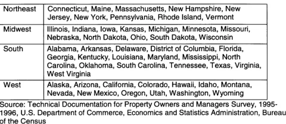
The data permits analysis at either the property or unit level. Information about the location of each property is very limited. Properties are identified as in one of the four census regions (Northeast, Midwest, South and West), inside or outside the metropolitan area, and inside or outside the central city. States, metropolitan areas, and cities are not specified.
2 Savage, Howard, 'What We Have Learned About Properties, Owners and Tenants From the 1995 Property Owners
and Managers Survey," U.S. Census Bureau, census website: http://www.census.gov:80/hhes/www/housing/poms/staterep4html. 3
Property Owners and Managers Survey Technical Documentation, U.S. Department of the Commerce, Washington
D.C.: February, 1997.
4 Properties used primarily for vacation homes were also excluded. Note that properties built or converted to rental
Table 3.1: Census Regions
Northeast Connecticut, Maine, Massachusetts, New Hampshire, New Jersey, New York, Pennsylvania, Rhode Island, Vermont Midwest Illinois, Indiana, Iowa, Kansas, Michigan, Minnesota, Missouri,
Nebraska, North Dakota, Ohio, South Dakota, Wisconsin South Alabama, Arkansas, Delaware, District of Columbia, Florida,
Georgia, Kentucky, Louisiana, Maryland, Mississippi, North Carolina, Oklahoma, South Carolina, Tennessee, Texas, Virginia, West Virginia
West Alaska, Arizona, California, Colorado, Hawaii, Idaho, Montana, Nevada, New Mexico, Oregon, Utah, Washington, Wyoming
Source: Technical Documentation for Property Owners and Managers Survey, 1995-1996, U.S. Department of Commerce, Economics and Statistics Administration, Bureau of the Census
The POMS collected information about the following aspects of rental housing:
* Ownership: characteristics of owners, ownership structure, attitudes toward the property, and reasons for owning.
* Property and unit characteristics: including age of structure, amenities, and recent capital improvements. Also, estimations of current value, value relative to other properties, and recent changes in property value.
* Financial characteristics: including method of and reasons for acquiring the property, mortgage information. The data includes detailed operating income and expense information, including rents from both residential and commercial space, and itemized expenses from the previous year.
* Management policies: including procedures for handling maintenance, tenant screening and turnover.
* Governmental benefits and regulations: includes property benefits received, such as tax credits and abatements, and participation in the federal Section 8 rental housing subsidy program.
3.2 Descriptive Statistics
The following summary, unless otherwise specified, presents property-level information based on the entire data set of 5754 observations, and considers only properties with greater than one unit. This summary relies heavily on the U.S. Census report, "What We have Learned About
-
.-I lii . - --- _ - - - , m
Properties, Owners and Tenants From the 1995 Property Owners and Management Survey," by Howard Savage.5
Owner Characteristics
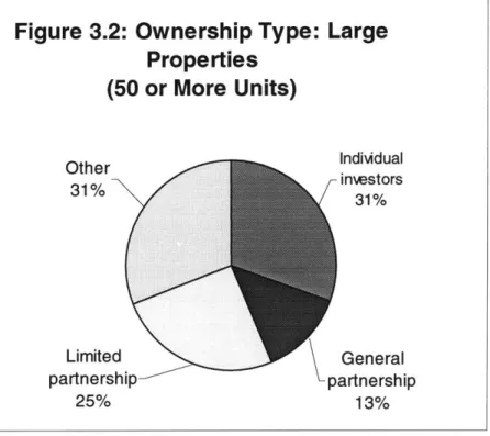
Most properties were owned by individual or partnership owners, half of whom owned only one property. However, the breakdown of ownership types varied considerably between small and large properties. Small properties were most likely to be owned by an individual, at 90 percent. In contrast, only 32 percent of the owners of properties with over 50 units were owned by individuals. (Figures 3.1 and 3.2) These properties also are more likely to be owned by partnerships (38%), corporations (11 %), or non-profits (6%). As of 1995, Real Estate
Investment Trusts (REITs) owned a negligible percentage (1%) of residential properties in the United States, but because their properties tend to be larger, this represents an estimated
417,612 units (2%).6
SSavage, 1.
Figure 3.2: Ownership Type: Large
Properties
(50 or More Units)
Other Individual 31% investors 31% Limited General partnership partnership 25% 13%About one fourth of multifamily properties were owner-occupied. This percentage decreased significantly at larger properties. Twenty-nine percent of small properties (less than 5 units) had owners living on the premises, while this was only true for 3% of properties with 50 or more units. Owners of large properties seemed more pleased with their properties, generally. Eighty-seven percent of owners of properties with 50 or more units reported that they would buy their property again. Meanwhile, only about two-thirds of small and medium-sized properties would buy their property again.
The primary reason investors acquired rental property was to receive income from rents, 33 percent. The second most common reason for acquisition was for use as a residence. Smaller properties were more likely to be bought for this purpose: a third of all properties under 5 units were purchased for use as a residence. Only 10% of all owners purchased their property for long-term capital gain. However, 22% of properties over 50 units were acquired for this purpose.
Half of multifamily property owners were between 45 and 64 years old, 85 percent were white (94 percent for large properties), 8 percent were African American, 6 percent were Hispanic and 4 percent were Asian or Pacific Islander.
Property Characteristics
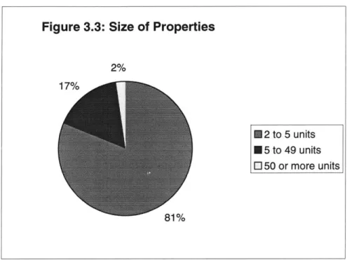
Although only 2% of all properties have 50 or more units, forty-six percent of all units were in properties with more than 50 units in 1995. (Figure 3.3)
Those units are more likely to be in a newer building. Properties with 50 or more units were built predominantly in the 1960's or later. (Table 3.2)
Table 3.2 - Property Location and Age
All Properties Properties with >4 units Properties with >49 units
Region # % # % # % Northeast 921,597 33% 139,545 27% 11,907 20% Midwest 682,289 25% 113,306 22% 10,093 17% South 562,232 20% 104,398 20% 19,356 32% West 588,748 21% 161,591 31% 18,220 31% 2,754,866 100% 518,840 100% 59,577 100% Decade Built Pre-1920 533,557 21% 66,822 14% 1,065 2% 1920 294,313 12% 45,979 10% 2,491 4% 1930 255,175 10% 28,975 6% 1,012 2% 1940 262,778 10% 32,730 7% 1,567 3% 1950 259,099 10% 42,111 9% 2,361 4% 1960 299,998 12% 83,827 18% 11,464 20% 1970 332,774 13% 88,322 19% 20,267 35% 1980 256,204 10% 73,252 15% 15,735 27% 1990 53,288 2% 12,743 3% 2,158 4% 2,547,187 100% 474,760 100% 58,121 100%
Note: Fewer units represented due to age non-responses.
Figure 3.3: Size of Properties
2%
E2 to 5 units
05 to 49 units 5 50 or more units
While 53% of all properties were built prior to 1960, only 15% of properties with 50 or more units were built before then.
The larger properties are also more likely to be located in the south or the west. While the northeast and midwest hold 58% of all properties, they only hold 37% of those properties with 50 or more units.
The distribution of properties among census regions was relatively uniform, with the largest number of properties in the south. Just over half of all properties were located in central cities, and only 10 percent were outside of metropolitan areas. The northeast was the most urban, with 56 percent of properties located in central cities. Of the four regions, the midwest is the least urban, with less than half of all properties located in central cities and 16 percent located in rural areas.
The most common capital improvements during the years 1990 to 1995 were bathroom renovations, kitchen facility replacements, and heating system upgrades.7 Only 12 percent of properties included handicap-accessible units.
According to owners, 38 percent of properties housed mostly low-income people, and 39 percent were occupied by mostly middle-income people. Only 3 percent of multifamily properties have mostly high-income renters, and these renters are more likely to be in
properties with more units. According to a report by the U.S. Department of Housing and Urban Development based on the POMS data, roughly half of multifamily units qualify as affordable according to HUD standards.8
Financial Characteristics
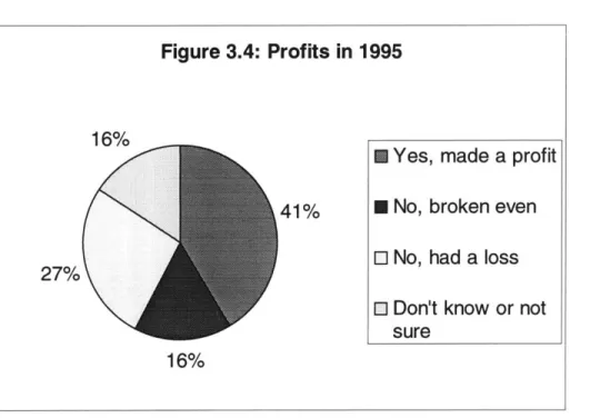
Fifty-eight percent of multifamily properties made a profit or broke even, and 27 percent had a loss. Sixteen percent of those surveyed didn't know if the property was profitable during the
7" Property Taxes and Parking Restrictions Were Leading Complaints of Multifamily Property Owners, Census Bureau Says," Press release, U.S. Department of Commerce, Census Bureau, December 2, 1998
"The Providers of Affordable Housing." U.S. Housing Market Conditions, 4 Quarter 1996, U.S. Department of
Housing and Urban Development, Office of Policy Development and Research, February 1997. Affordable rental units are identified as those that a family with 50 percent of the HUD-adjusted median income could afford witrhout spending more than 30 percent of their income on rent.
previous year.9 Only 3 percent of properties over 50 units reported losses, but a high 37 percent reported that they didn't know whether the property was profitable. Researchers from the National Multihousing Council point out that this may be because the interviews were done in early 1996, before the previous year's profitability was determined.10 (Figure 3.4)
16%
27%
Figure 3.4: Profits in 1
k
41%
16%
Operating income and expenses vary widely among properties. Average rent receipts per unit
were $5,152.11 Based on property level data, yearly median operating expenses per unit were
$2,300. Large properties had higher median operating expenses as $3,300. Three-quarters of units are in mortgaged properties. Average mortgage expenses were $1,139 per unit, or 22 percent of rent receipts.
Management Policies
About 21 percent of owners reported that they were seeking new tenants at the time of the survey. Approximately one-quarter of properties with less than 5 units rejected tenants in the
9 "Property Taxes and Parking Restrictions Were Leading Complaints of Multifamily Property Owners, Census Bureau
Says," Press release, U.S. Department of Commerce, Census Bureau, December 2, 1998
10 "Highlights from HUD's New Survey of Property Owners and Managers," Research Notes, National Multihousing
Council, February 1997.
Emrath, Paul, "Property Owners and Managers Survey," Housing Economics, July 1997: (6 -9), p. 7. " Yes, made a profit " No, broken even
E No, had a loss El Don't know or not
last two years, and 85 percent of properties with 50 or more units. The main reasons tenants were rejected for apartments were poor credit, insufficient income, and unfavorable references.
Fifty-five percent of the owners of multifamily properties were attempting to reduce tenant turnover by redecorating or making other improvements. Twenty-seven percent of properties offered rent concessions to retain residents. Larger properties were more likely to offer increased services as a means to retain tenants. Owners at less than 1 percent of properties were trying to increase tenant turnover.
The median amount of gross rental income spent on maintenance was 14%. Smaller properties spent a smaller percent of income on maintenance.12
Governmental Benefits and Regulations
Overall, 7 percent of properties have Section 8 tenants, with larger properties more likely to participate in the Section 8 program. Four percent of properties participated in other Federal, state, or local housing programs. Owners of larger properties were much more likely to know about the Section 8 program, at 88 percent. Nearly half of small multifamily property owners did not know about the program.
When asked what governmental regulations made it more difficult to operate the property, property taxes were consistently ranked highest, regardless of size of property. Parking was also listed as a major complaint.
3.3 Response Limitations
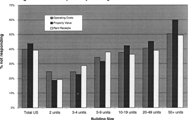
Important considerations in analyzing the data are the rate and pattern of non-response to the survey questions. Few categories were completed by all respondents and many fundamental questions had high rates of non-response. Financial information, in particular, was frequently not reported. Per Census tabulations by unit, 40% of represented units did not have complete operating cost data." The category most responded to, advertising cost, had a 38%
non-response rate. Six of the twenty operating cost categories had over 50% non-non-response rates. When tabulated by property size, the larger the property, the less likely the owner was to
respond to operating cost questions. (Figure 3.5) Tabulation of the survey responses revealed
12 Savage, 2.
only 32% of individual owners responded to all sixteen operating cost categories used in
calculating net operating income in this paper. This was slightly better than the response rate of properties owned by limited partners (29%) and much better than the response rate of real estate corporations (18%), the next largest owner types. This is consistent with the tendency for limited partnerships and real estate corporations to own larger properties.
Figure 3.5: Non-response by Building Size 70% 60% - Operating Costs Property Value [3 Rent Receipts g 50% 0% 0 1. 40% 0 0 C 30% 20% 10%
Total US 2 units 3-4 units 5-9 units 10-19 units 20-49 units 50+ units
Chapter 4: POMS and Capital Improvements
To begin to understand the determinants of renovation, basic characteristics are investigated in search of obvious relationships. The building's size, age, location, ownership, profitability and tenant composition are all potentially significant variables in the probability of its renovation and shall be explored in this chapter with bivariate correlations.
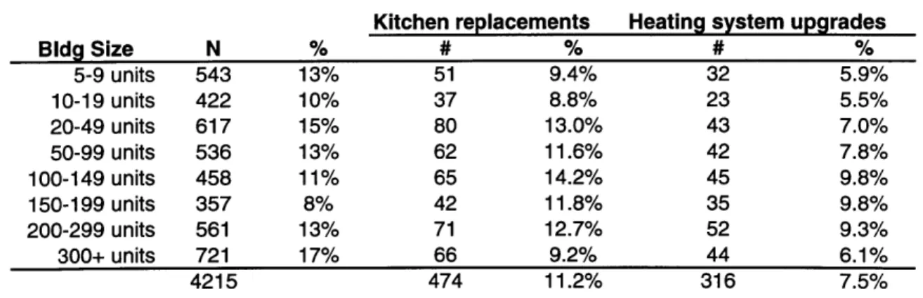
To begin, we look at the effect of property size on its likelihood to be renovated. The series of capital improvement questions in POMS ask if any improvements were made to the property, not the subject unit. This means that the question would be responded to in the affirmative if any unit in the property had had a kitchen replaced, for example, in the last five years. Obviously, then, the more units in a property, the greater the likelihood work had been done. Unfortunately, the relationship is not direct. Several units in a property may be remodeled at once, for example. Also, other capital improvement items, such as the plumbing and air tempering systems, may serve the whole property resulting in a likelihood of replacement less directly related to the number of units in the property. Table 4.1 shows that, in fact, no clear
relationship exists for either an appearance-related item, a kitchen, or a basic system, heat. For both the largest and smallest properties, the rate of remodel is somewhat lower, but the
expected increase with size is not evident.
Table 4.1 - Effect of Building Size on Renovation
Kitchen replacements Heating system upgrades
Bldg Size N % # % # % 5-9 units 543 13% 51 9.4% 32 5.9% 10-19 units 422 10% 37 8.8% 23 5.5% 20-49 units 617 15% 80 13.0% 43 7.0% 50-99 units 536 13% 62 11.6% 42 7.8% 100-149 units 458 11% 65 14.2% 45 9.8% 150-199 units 357 8% 42 11.8% 35 9.8% 200-299 units 561 13% 71 12.7% 52 9.3% 300+ units 721 17% 66 9.2% 44 6.1% 4215 474 11.2% 316 7.5%
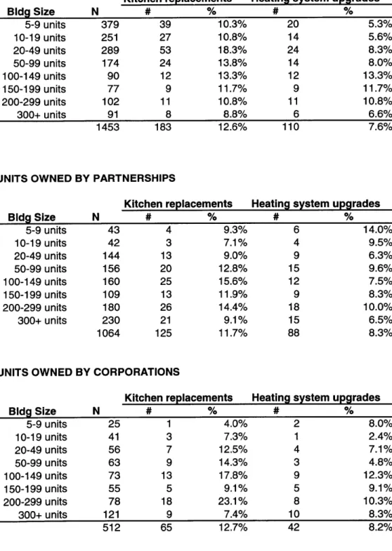
As mentioned, the individual property owner owns a greater percentage of smaller properties, while corporations and partnerships own a greater percentage of larger properties. To see if differing behavior of these types of owners could have some relation to renovation probability,
we separate them out in Table 4.2. Again, no clear pattern is evident between likelihood to remodel and building size for each type of owner. The smallest and largest properties typically have lower rates, but high and low spikes exist throughout the data. A low number of
observations in some categories contributes to this.
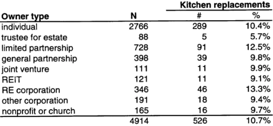
When looking at a summary of remodeling rates for most owner types, little variation exists except of that of real estate corporations and limited partnerships. See Table 4.3. Whereas other entities renovated kitchens approximately 10% of the time, these two major owners
renovated slightly more than 12% of the time.
A possible explanation for this might be that their specialization in real estate gives them the ability to recognize the profit maximizing opportunity. A REIT may have similar knowledge but may have funding problems due to the cash payout requirements of their structure. General partnerships and joint ventures may have control issues. The individual owner is the third most likely to remodel. Their ability to recognize and fund the opportunity probably varies more widely. Many other explanations are possible, though, and the differences are not overly significant.
Table 4.2 - Ownership and Size Interactions UNITS OWNED BY INDIVIDUALS
Kitchen replacements Heating system upgrades
Bldg Size N # % # % 5-9 units 379 39 10.3% 20 5.3% 10-19 units 251 27 10.8% 14 5.6% 20-49 units 289 53 18.3% 24 8.3% 50-99 units 174 24 13.8% 14 8.0% 100-149 units 90 12 13.3% 12 13.3% 150-199 units 77 9 11.7% 9 11.7% 200-299 units 102 11 10.8% 11 10.8% 300+ units 91 8 8.8% 6 6.6% 1453 183 12.6% 110 7.6%
UNITS OWNED BY PARTNERSHIPS
Kitchen replacements Heating system upgrades
Bldg Size N # % # % 5-9 units 43 4 9.3% 6 14.0% 10-19 units 42 3 7.1% 4 9.5% 20-49 units 144 13 9.0% 9 6.3% 50-99 units 156 20 12.8% 15 9.6% 100-149 units 160 25 15.6% 12 7.5% 150-199 units 109 13 11.9% 9 8.3% 200-299 units 180 26 14.4% 18 10.0% 300+ units 230 21 9.1% 15 6.5% 1064 125 11.7% 88 8.3%
UNITS OWNED BY CORPORATIONS
Kitchen replacements Heating system upgrades
Bldg Size N # % # % 5-9 units 25 1 4.0% 2 8.0% 10-19 units 41 3 7.3% 1 2.4% 20-49 units 56 7 12.5% 4 7.1% 50-99 units 63 9 14.3% 3 4.8% 100-149 units 73 13 17.8% 9 12.3% 150-199 units 55 5 9.1% 5 9.1% 200-299 units 78 18 23.1% 8 10.3% 300+ units 121 9 7.4% 10 8.3% 512 65 12.7% 42 8.2%
Table 4.3 - Renovation by Owner Type
Owner type
individual
trustee for estate limited partnership general partnership joint venture RE T RE corporation other corporation nonprofit or church N 2766 88 728 398 111 121 346 191 165 4914 Kitchen 289 5 91 39 11 11 46 18 16 526 replacements 10.4% 5.7% 12.5% 9.8% 9.9% 9.1% 13.3% 9.4% 9.7% 10.7%
Another obvious influence to investigate is age. Table 4.4 shows the possible existence of differing bivariate relationships for the remodel of appearance and systems items.
Table 4.4 - Renovation by Structure Age
Kitchen replacements Heating system upgrades
Year Built N # % # % <1919 527 52 9.9% 41 7.8% 1920-1929 366 36 9.8% 36 9.8% 1930-1939 268 27 10.1% 14 5.2% 1940-1949 298 32 10.7% 19 6.4% 1950-1959 376 48 12.8% 33 8.8% 1960-1969 902 127 14.1% 99 11.0% 1970-1979 1374 184 13.4% 123 9.0% 1980-1984 491 39 7.9% 17 3.5% 1985-1989 675 30 4.4% 22 3.3% 5277 575 10.9% 404 7.7%
The rate of kitchen remodeling increases with age to a high point in structures approximately 20 to 30 years old. The rate diminishes slightly in structures older than that. Rate of heating
system upgrade has distinct high points in structures 30 and 70 years old. As Mayer showed, the inadequacy of basic systems decreases the likelihood of remodeling on the whole. Basic systems are replaced when they must be for functional reasons. The pattern of heating system upgrade suggests a lifespan of a heating system of approximately 30 to 40 years. Kitchen remodeling occurs more frequently as styles and their appeal change.
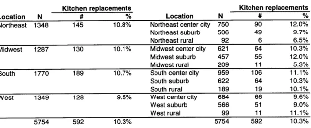
Location may also be related to renovation. The POMS data specifies only whether the
property is in the Northeast, Midwest, South or West, whether it is in a metropolitan area, and, if so, whether it is in the center city.
Table 4.5 - Renovations by Location
Kitchen replacements Kitchen replacements
Location N # % Location N # %
Northeast 1348 145 10.8% Northeast center city 750 90 12.0%
Northeast suburb 5v6 49.7%
Northeast rural 92 6 6.5%
Midwest 1287 130 10.1% Midwest center city 621 64 10.3%
Midwest suburb 457 55 12.0%
Midwest rural 209 11 5.3%
South 1770 189 10.7% South center city 959 106 11.1%
South suburb 622 64 10.3%
South rural 189 19 10.1%
West 1349 128 9.5% West center city 684 66 9.6%
West suburb 566 51 9.0%
West rural 99 11 11.1%
5754 592 10.3% 5754 592 10.3%
Looking at the rate of remodel of kitchens by just region of country
and west - shows that the rate of kitchen remodel is fairly uniform.
slightly below the rest of the group, as one might expect given the
- northeast, midwest, south
The rate in the west is
newer housing stock there.
The northeast and south have the highest rate. When each region is divided into center city,
suburb and rural areas, differences are still slight, but a pattern is evident. In the northeast and
midwest, the remodeling rates are much higher in the metropolitan areas than the rural areas.
In the south and west, the remodeling rates are more uniform across the divisions. It is
important to note that the rural data contains much fewer observations, though. One possible
explanation for the different rates is in the definition of metropolitan area. Western and southern
metropolitan areas extend to areas that are essentially rural. The difference in age between
housing in and out of the metropolitan area is probably lower in the south and west as well.
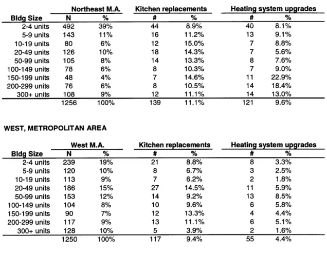
Since the larger buildings are located more frequently in the west and smaller buildings in the northeast, we again check if the remodel rate's variation with size is more clearly related if we
separate out the regions. See Table 4.6. Again, no clear relationship is evident and the small sample size for some categories gives more deviation than probably exists.
Table 4.6 - Renovation by Size and Location NORTHEAST, METROPOLITAN AREA
Northeast M.A. N % 492 39% 143 11% 80 6% 126 10% 105 8% 78 6% 48 4% 76 6% 108 9% 1256 100% Kitchen replacements 44 8.9% 16 11.2% 12 15.0% 18 14.3% 14 13.3% 8 10.3% 7 14.6% 8 10.5% 12 11.1% 139 11.1%
Heating system upgrades 40 8.1% 13 9.1% 7 8.8% 7 5.6% 8 7.6% 7 9.0% 11 22.9% 14 18.4% 14 13.0% 121 9.6%
WEST, METROPOLITAN AREA
Bldg Size 2-4 units 5-9 units 10-19 units 20-49 units 50-99 units 100-149 units 150-199 units 200-299 units 300+ units West M.A. N % 239 19% 120 10% 113 9% 186 15% 153 12% 104 8% 90 7% 117 9% 128 10% 1250 100% Kitchen replacements 21 8.8% 8 6.7% 7 6.2% 27 14.5% 14 9.2% 10 9.6% 12 13.3% 13 11.1% 5 3.9% 117 9.4%
Heating system upgrades
8 3.3% 3 2.5% 2 1.8% 11 5.9% 13 8.5% 6 5.8% 4 4.4% 6 5.1% 2 1.6% 55 4.4%
Since the renovation decision is one of profit maximization, financial characteristics should have some relation to its likelihood. A most basic financial characteristic is profitability. Table 4.7
shows the respondent's rate of remodel given the profitability reported. For both an
appearance-oriented item and a basic system, the rates are higher if the owner does not think the property was profitable the previous year. One possible explanation is that the work was done to increase profitability.
Bldg Size 2-4 units 5-9 units 10-19 units 20-49 units 50-99 units 100-149 units 150-199 units 200-299 units 300+ units
Table 4.7 - Renovation by Profitability
Kitchen replacements Heating system upgrades
Profitability # % # %
yes 1798 199 11% 110 6%
no, broke even 265 41 15% 27 10%
no, had a loss 576 77 13% 64 11%
don't know or not sure 1252 139 11% 98 8%
not reported 324 18 6% 17 5%
4215 474 11% 316 7%
Another is that the property was not profitable because of the construction costs incurred and rent lost by renovating. This cannot be a clear determinant of the likelihood to remodel, then.
Tenant income characteristics provide a glimpse into the property's market position, and its structure and neighborhood quality. A breakdown of renovation rates by tenant income shows a slight increase in renovations in properties with low income tenants, whether exclusively low income or a mix. See Table 4.8. Mayer's study showed that renovation was more likely in neighborhoods with higher crime rates and in buildings in poor condition visually. This would be one explanation of the higher remodel rates, if these factors are what is making the property affordable. The mixed income properties that included high income tenants also had high renovation rates, though, indicating that other factors must be at work. In any event the differences in rate are slight.
Table 4.8 - Renovation by Incidence of Crime Kitchen replacements Vandalism N # % never 2469 227 9.2% rarely 1796 199 11.1% sometimes 906 122 13.5% frequently 189 21 11.1% 5360 569 10.6%
Examination of physical, geographic, management, financial and tenant characteristics reveals some weak bivariate correlations to the renovation rate of rental housing, but no clear
determinants. In the next chapter, more significant relationships will be sought through multivariate analysis.
Chapter 5: Multivariate Analysis
5.1 Description of the Model
In this chapter, multivariate analysis is performed to better understand the determinants of the decision to renovate. Since no information was collected in the POMS on expenditures for capital improvements, we are limited to exploring only whether capital improvements were made, not amount spent. Given the exploratory nature of this study and the limitations of the data set, this is a reasonable starting point.
The lack of any quantification of value of the improvement immediately raises the question of whether all the reported improvements were actually substantial. The POMS includes questions about both repairs and maintenance and capital improvements. For both, questions were asked about whether work was done in the last five years for a number of similar categories. For example:
Repair and maintenance section:
10. In the last five years, was any of the following work done to the rental unit identified in Item A?
c. Some or all kitchen appliances replaced.
Capital improvement section:
19. In the last five years have any of the following capital improvements or upgrades been made or started at this property? Capital improvements are additions to the property that increase the value or upgrade the facilities.
d. Replacement of kitchen facilities.
In addition, the amount spent on repairs and maintenance was quantified in two ways. In the operating cost section, an item was included for repairs and maintenance expenditures. The question prior to this asked for the percentage of rental income spent on maintenance. Both questions clearly stated that expenditures for capital improvements were to be excluded.
Given that similar questions were posed but with a clear difference in magnitude of scope and given that the difference was reinforced whenever maintenance expenditures were requested, it
is assumed that the respondents only indicated true, substantial capital improvements in that section. Minor repairs are assumed to have been properly indicated in the maintenance and
repair section.
A linear equation was estimated using an ordinary least squares regression.
I =a + SUM(Bi*Xi)
Where I = 1 if subject improvement was made in 1995, 0 if not. a = constant
Bi = Coefficients estimated in the regression.
Xi = Variables hypothesized to affect the likelihood of the improvements being made.
Only improvements made in 1995 are being used since several variables give conditions existing at the property in 1995 or the year previous. These conditions could have been very different prior to any remodeling done before 1995. Equations are fit for four different
improvement types. The replacement of kitchens and bathrooms is viewed as a more
discretionary improvement, while the upgrade of the plumbing and heating systems is less so. Fitting an equation for all four should draw out both general and type-specific determinants.
The observations used were limited to those of properties with greater than four units.
Properties smaller than these are frequently owner-occupied and sometimes treated differently by lending institutions. As discussed, homeowner renovation decision behavior is different than rental owner behavior. In properties this small, the owner-occupied behavior may dominate and skew the results. Of the 5754 observations in POMS, 4215 represent properties larger than four units in size.
Rural properties were also excluded from the empirical analysis. The crosstabulations presented in the previous chapter showed that, in some regions, renovation behavior differed between metropolitan and rural areas. The rural areas also contained far fewer observations.
Given their potentially confounding effects and small numbers, their loss was viewed as acceptable. This narrowed the dataset to 3884 observations.
As mentioned earlier, the rate of non-response to some questions in the survey was very high. While the capital improvement questions were responded to very frequently, the equation estimated includes variables with higher non-response rates. Of the 3884 multifamily, metropolitan observations, only 1534 observations had complete information in all of the categories of interest. Tables 5.1 and 5.2 list the descriptive statistics for all reported values of each item and those of the dataset used in the regression analysis, respectively. Comparison of the two shows some differences. All of the tested capital improvements tested occurred more frequently in regression sample. More of the properties were profitable, a higher percentage of real estate corporate owners is represented, and fewer properties employ managers. The tested sample has an older mix of smaller buildings. More properties with low and moderate to low income tenants are included. Slightly more midwestern and western properties are included in the reduced set at the expense of southern properties. The tested set contains a much higher percentage of rent controlled units. Overall, though, the differences are small and acceptable for the level of analysis undertaken. Given the reduced sample size, dividing the sample further was resisted, though. Regional effects were handled with both region dummy variables and select interaction terms.
The following are a series of hypotheses regarding the effect of various conditions on the likelihood of renovation. Characteristics of the financial condition, owner, management, tenant, structure and neighborhood are tested. Hypotheses of previous researchers are tested
alongside new hypotheses.
5.2 Specific Hypotheses Financial characteristics
Profitability
The property's profitability over the previous year may have some relation to whether a profit maximizing opportunity was pursued. The most likely candidate for improvement is the property that is not profitable. The owner of the profitable property may not be actively pursuing ways to further increase profitability. While the owner of the unprofitable property may be reluctant to
Table 5.1 - Descriptive Statistics for All Respondents a
N Min. Max. Mean Std. Dev. Dependent Variable
Kitchen replacement 3731 0
Bathroom replacement 3728 0
Plumbing replacement 3743 0
Heating system replacement 3748 0
Financial Characteristics
Property profitable last year 3591 0
Property more profitable than similar properties 3639 0 10%-19% of tenants delinquent 3154 0
20% or more of tenants delinquent 3154 0
*Omitted - Less than 10% of tenants delinquent
Value increased 3669 0
Ownership Characteristics
Owner purchased within past 2 years 2886 0
Owner intends to hold property for 5 or more years 2771 0
Individual owner 3223 0
Individual owner in the midwest 3223 0
Individual owner in the south 3223 0
Individual owner in the west 3223 0
Real estate corporation 3223 0
*Omitted - Limited partner or other owner Management Characteristics
Owner employs manager 3746 0
Competes for tenants with subsidized properties 3521 0
Competes for tenants with public housing 3521 0
*Omitted - Competes with private, nonsubsidized only
10%-19% of rental income spent on maintenance 2621 0
20% or more of rental income spent on maintenance 2621 0
*Omitted - Less than 10% spent on maintenance
Physical Characteristics
Built prior to 1940 3722 0
Built 1940-1959 3722 0
Built 1960-1979 3722 0
*Omitted - Built 1980 or after
20-49 units 3884 0 50-99 units 3884 0 100-199 units 3884 0 200-299 units 3884 0 300+ units 3884 0 *Omitted - 5-19 units Neighborhood Characteristics Vandalism 3615 0 Theft 3594 0 Tenant Characteristics
Tenant income low or low to moderate 3668 0 Tenant income high or moderate to high 3668 0
Tenant income diverse 3668 0
*Omitted - Tenant income moderate
Lower tenant turnover desired 3622 0
Location North suburban 3884 0 Midwest urban 3884 0 Midwest suburban 3884 0 South urban 3884 0 South suburban 3884 0 West urban 3884 0 West suburban 3884 0
*Omitted - North urban
Rent control 3841 0
Rent control in the North 3841 0
a among properties with more than 4 units and in metropolitan areas
0.118 0.091 0.070 0.077 0.462 0.141 0.155 0.117 0.322 0.288 0.256 0.266 0.499 0.348 0.362 0.322 1 0.278 0.448 0.138 0.867 0.406 0.084 0.114 0.127 0.098 0.829 0.232 0.167 0.345 0.340 0.491 0.277 0.318 0.333 0.297 0.377 0.422 0.373 1 0.286 0.452 1 0.171 0.377 0.125 0.096 0.484 0.134 0.125 0.197 0.143 0.184 0.331 0.295 0.500 0.340 0.331 0.398 0.350 0.387 1 0.662 0.473 1 0.644 0.479 0.451 0.498 0.157 0.364 0.067 0.250 1 0.797 0.402 0.078 0.108 0.091 0.209 0.135 0.141 0.119 0.268 0.311 0.288 0.407 0.341 0.348 0.324 1 0.111 0.314 1 0.067 0.249
Table 5.2 - Descriptive Statistics - Multivariate Analysis Sample Set
N Min. Max. Mean Std. Dev. Dependent Variables
Kitchen replacement 1534
Bathroom replacement 1534
Plumbing replacement 1534
Heating system replacement 1534
Financial Characteristics
Property profitable last year 1534
Property more profitable than similar properties 1534
10%-19% of tenants delinquent 1534 20% or more of tenants delinquent 1534
*Omitted - Less than 10% of tenants delinquent
Value increased 1534
Ownership Characteristics
Owner purchased within past 2 years 1534 Owner intends to hold property for 5 or more years 1534
Individual owner 1534
Individual owner in the midwest 1534
Individual owner in the south 1534
Individual owner in the west 1534
Real estate corporation 1534
*Omitted - Limited partner or other owner
Management Characteristics
Owner employs manager 1534
Competes for tenants with subsidized properties 1534 Competes for tenants with public housing 1534
*Omitted - Competes with private, nonsubsidized only
10%-19% of rental income spent on maintenance 1534 20% or more of rental income spent on maintenance 1534
*Omitted - Less than 10% spent on maintenance
Physical Characteristics
Built prior to 1940 1534
Built 1940-1959 1534
Built 1960-1979 1534
*Omitted - Built 1980 or after
20-49 units 1534 50-99 units 1534 100-199 units 1534 200-299 units 1534 300+ units 1534 *Omitted - 5-19 units Neighborhood Characteristics Vandalism 1534 Theft 1534 Tenant Characteristics
Tenant income low or low to moderate 1534 Tenant income high or moderate to high 1534
Tenant income diverse 1534
*Omitted - Tenant income moderate
Lower tenant turnover desired 1534
Location North suburban Midwest urban Midwest suburban South urban South suburban West urban West suburban
*Omitted - North urban Rent control
Rent control in the North
1534 1534 1534 1534 1534 1534 1534 0.137 0.104 0.091 0.083 0.548 0.149 0.159 0.127 0.344 0.305 0.287 0.277 0.498 0.356 0.366 0.333 0 1 0.284 0.451 0.114 0.841 0.396 0.090 0.085 0.127 0.070 0.763 0.253 0.199 0.318 0.366 0.489 0.286 0.280 0.333 0.255 0.425 0.435 0.400 1 0.308 0.462 1 0.166 0.372 0.178 0.110 0.460 0.161 0.118 0.185 0.126 0.151 0.383 0.313 0.499 0.368 0.323 0.389 0.332 0.358 1 0.668 0.471 1 0.636 0.481 0.520 0.126 0.055 0.500 0.332 0.229 1 0.780 0.415 0.076 0.124 0.093 0.179 0.106 0.152 0.113 0.266 0.330 0.291 0.383 0.308 0.359 0.316 1534 0 1 0.179 0.384 1534 0 1 0.098 0.297
invest more in it, or may have problems funding the project, he should still be more actively pursuing such options. A true interpretation is muddied by the possibility that the property was unprofitable because of the expenses involved in the capital improvement. A dummy variable is set equal to one if the respondent reported earning a profit the previous year. The omitted case is the owner not making a profit or unsure of his profitability.
Relative profitability
Two possible effects are possible. An owner who feels his property is not as profitable as comparable properties is more likely to remodel to improve its competitiveness. Alternatively, though, an owner who just committed capital to his building is probably convinced it is at its optimal condition and more profitable than its competitors. A dummy variable equal to one if the respondent thought the property more profitable than similar properties will help clarify the issue.
Change in property values
A change in property values in itself does not mean that a profit maximizing opportunity exists. It does provide the liquidity to fund any opportunities that do exist, though. Borrowing against the newfound value allows the owner to undertake any worthwhile projects. A dummy variable
is set equal to one if the respondent thought area property values had risen in the past year.
Delinquency
Tenant delinquency in rent payments at low levels is an expected but unwelcome cost of ownership. At low levels, the cost of removing tenants is unjustified. Beyond a certain point, it becomes worthwhile to seek better tenants. Renovation is hypothesized to be one way this is done. Higher delinquency may spur property owners to reposition the property through
improvement. When delinquency rates become too high, however, a cash flow problem arises. Two dummy variables are used to test for this effect. The first is set equal to one when
delinquencies are between 10% and 19%, the other when they are 20% or greater.
Cash Flow and Cost of Capital
Besides the respondent's answer to the profitability question, profitability can be calculated from the financial information given. Measures of profitability were calculated from the rent receipts, operating costs, mortgage payments and value. These included net operating income to value