Critical electric field quantification for inducing bacterial electroporation

Critical Electric Field Quantification for Inducing

Bacterial Electroporation

by

Sijie Chen

B.S., B.Econ., Peking University (2017)

Submitted to the Department of Mechanical Engineering

in partial fulfillment of the requirements for the degree of

Master of Science in Mechanical Engineering

at the

MASSACHUSETTS INSTITUTE OF TECHNOLOGY

June 2019

@

Massachusetts Institute of Technology 2019. All rights reserved.

Signature redacted

Author ...

Department of Mechanical Engineering

May 18, 2019

Certified by...Signature

Accepted by ..

JUN

13 2019

LIBRARIES

redacted

Cullen Buie

Associate Professor

Thesis Supervisor

Signature redacted

...

NicolAs Hadjiconstantinou

Graduate Officer, Department of Mechanical Engineering

Critical Electric Field Quantification for Inducing Bacterial

Electroporation

by

Sijie Chen

Submitted to the Department of Mechanical Engineering on May 18, 2019, in partial fulfillment of the

requirements for the degree of

Master of Science in Mechanical Engineering

Abstract

Electroporation is one of the most popular methods for rapid and efficient intracellu-lar transport of foreign molecules, such as peptides, drugs, and DNA, and is crucial for applications in genetic engineering. However, there is still a lack of mechanistic understanding of electroporation, and the most common method to optimize electro-poration parameters for bacterial genetic transformation is still based on trial and error. In this work, to alleviate this issue we use microfluidic techniques to achieve rapid screening of electric fields for electroporation in live bacteria. To determine the critical electric field required for inducing bacterial electroporation, we extend upon a previously developed microfluidic assay. By quantifying the critical electric field

values of gram-positive bacteria Corynebacterium glutamicum and Bacillus subtilis

168, and the gram-negative bacteria Escherichia coli BL21 (DE3) and Pseudomonas

syringae ESC 10 in 10% glycerol and 0.01x PBS, we study the effects of using

dif-ferent buffer solutions for difdif-ferent bacteria in the electroporation process. We also investigate the relationship between cell polarizability and critical electric field for these cells in the aforementioned buffer solutions. Next, we discuss the accuracy of the measurement by illuminating how undesired phenomena such as electroosmosis and electrophoresis contribute to the measurement error. Results of this study will enhance our understanding of the electroporation process and provide insights in discovering and optimizing electroporation protocols.

Thesis Supervisor: Cullen Buie Title: Associate Professor

Acknowledgments

I would like to express my greatest appreciation towards my advisor, Professor Cullen Buie, who has provided me generous support and guidance throughout these two years. From him, I not only learned how to do well in academia, but also learned how to be a person with virtues, e.g. wit, truthfulness, fairness, friendliness, etc..

I would also like to thank the members of the Laboratory for Energy and Mi-crosystems Innovation (LEMI). Thanks to Dr. Qianru Wang for her inspiration and help in this project, who taught me a lot of skills on doing experiments with bacteria, and I am deeply impressed by her passion and rigorous attitude on research; Dr. Paulo A. Garcia and Rameech McCormack for teaching me the skills on electropora-tion experiments; Dr. Zhifei Ge for his advice and suggeselectropora-tions on research topics; Dr. Chris Vaiana, Dr. Chelsea Catania, Dr. Kameron Conforti, and Laura M. Gilson for all the inspiring discussions; Hyungseok Kim for facing all the difficulties together; as well as Dr. Andrew D. Jones III and our administrator Maral Banosian.

I must pay particular thanks to my dear parents, Changsheng Chen and Hongying Chen. Though they are not in the U.S. with me, their understanding, encouragement, and support always give me the strength to overcome all the challenges.

Contents

1 Introduction

1.1 Genetic Engineering Overview . . . .

1.2 Gene Delivery Overview . . . .

1.3 Electroporation Overview . . . .

1.4 Purpose of the Research . . . .

1.5 Thesis Organization . . . .

2 Microfluidic Screening of Electric Fields for Electroporation

2.1 Introduction . . . .

2.2 Fundamental Principles of the Device . . . .

2.3 Determination of Critical Electric Field . . . .

3 Microfluidic Electroporation Assay Experimental Design

3.1 Introduction . . . . 3.2 3.3 3.4 3.5 M ethods . . . .

3.2.1 Culture Conditions for Bacterial Strains . . . .

3.2.2 Electroporation Protocol and Image Data Collection

Experiment Results . . . . Results Analysis and Conclusions . . . . Cell Polarizability and Critical Electric Field . . . .

4 Analysis of Undesired Phenomenon during Electric Field Measure-ments 13 13 14 15 17 17 19 19 19 22 27 . . . . . 27 . . . . . 28 . . . . . 28 . . . . . 28 . . . . . 29 . . . . . 33 . . . . . 36 39

4.1 Introduction . . . . 39

4.2 Electroosmosis and Electrophoresis . . . . 39

4.3 Contradiction between Methods for Critical Electric Field Determination 42

5 Conclusions and Future Work A Supplemental Figures B C Supplmental Table 47 49 55 59

List of Figures

2-1 Representative electric field distribution in microfluidic assay device 21

2-2 Method I for the determination of critical position . . . . 24

2-3 Method II for the determination of critical position . . . . 25

3-1 Measured critical electric field for Corynebacterium glutamicum in

dif-ferent buffer solutions . . . . 30

3-2 Measured critical electric field for Bacillus subtilis 168 in different

buffer solutions . . . . 31

3-3 Measured critical electric field for Escherichia coli BL21 (DE3) in

dif-ferent buffer solutions . . . . 32

3-4 Measured critical electric field for Pseudomonas syringae ESC 10 in

different buffer solutions . . . . 33

3-5 Measured critical electric field for different strains in different buffer

solutions . . . . 35

3-6 Correlation between critical electric field and cell polarizability . . . . 38

4-1 Cell shift caused by electroosmosis and electrophoresis . . . . 41

4-2 Using Method I and Method II to determine the critical electric field 43

4-3 Fluorescence intensity before and after the pulse along the channel . 44

4-4 Clusters of cells moving leftward . . . . 45

A-i Results of "normplot()" function in Matlab for the gram-positive bacteria 49 A-2 Results of "normplot()" function in Matlab for the gram-negative

A-3 Results of "normplot(" function in Matlab for the Escherichia coli

BL21 (DE3) in 0.01 x PBS after discarding outlier data . . . . 51

A-4 Measured cell polarizability of four strains in different buffers using

3DiDEP device. . . . . 52

A-5 Measured cell shape of four strains in different buffers using 3DiDEP

List of Tables

Chapter 1

Introduction

1.1

Genetic Engineering Overview

Genetic engineering, also called genetic modification or genetic manipulation, refers to the process of inserting new genetic information into existing cells in order to modify a specific organism for the purpose of changing its characteristics [1]. It is comprised of a set of technologies for gene manipulation, for gene delivery, and for gene targeting. Specifically, after obtaining new DNA by artificial synthesis or by isolating and copying the genetic material of interest using gene manipulation techniques, the DNA can be inserted into host organisms via gene delivery methods. The modification takes effect when the nucleic acid sequence is inserted randomly or targeted to a specific location of the genome. In addition to inserting genes, the

process can be used to remove, or "knock out", genes

[21.

Though both genetic engineering and conventional breeding are used for obtaining organisms with desired phenotype, they are profoundly different. As conventional breeding usually involves crossing together organisms with relevant characteristics and selecting the offspring with desired characteristics, the essential of the whole process is selection, so only the expression of genetic material which is already present within a species can be achieved. As genetic engineering takes the gene directly from one organism and inserts it in the other, the essential of the whole process of genetic engineering is insertion, which is much more efficient and can be used to insert any

genes from any organism, even ones from different domains.

As the genetic engineering can be used for different organisms, including bacteria, viruses, animals, and plants, it has led to applications in numerous fields such as medicine, agriculture, gene therapy, and industrial biotechnology. In 1974, the first genetically modified animal was created by Rudolf Jaenisch via inserting DNA into

mouse

131.

engineered human insulin [4, 5]. The first genetically modified plant was produced

in 1983 [6], and the first genetically modified food approved for release was the Flavr Savr tomato in 1994 [7]. Up to now, genetic engineering has become a more and more powerful tool. By knocking out genes responsible for certain conditions, it is possible to create animal model organisms of human diseases, which not only gives birth to hormones, vaccines, and other drugs [81, but also enables the curing of genetic diseases through gene therapy. By utilizing genetic engineering, the yield potential, quality and disease resistance in crops can be significantly improved [9]. The same techniques

can also be used for industrial applications, e.g. enzymes for laundry detergent

110].

1.2

Gene Delivery Overview

Gene delivery is the process of introducing foreign genetic material, such as DNA or RNA, into host cells 111]. It is a necessary step in genetic engineering, as genetic ma-terial must reach the nucleus of the host cell to induce gene expression [12]. Usually this process requires making the cell membrane permeable using some intervention technologies so that the foreign genetic materials can be inserted through the mem-brane into the hosts genome in a stable manner. Even for some bacteria that can naturally be able to take up foreign DNA without external methods, using gene deliv-ery technologies can make this process more efficient [13]. It's worth pointing out that the process of delivering genes into bacteria or plants is more frequently called trans-formation. When delivering genes into animals, the process is called transfection, as transformation has a different meaning in relation to animals, indicating progression to a cancerous state [14].

To ensure the gene been delivered successfully, it is crucial to keep the foreign genetic material stable with high efficiency throughout the whole delivery process. Hence, people usually synthesize the foreign DNA to be a part of a vector. The vectors designed for this purpose can be divided into two categories, recombinant viruses and synthetic vectors, the so-called viral and non-viral vectors [12, 151. Viruses can serve as effective vehicles because the viral genome can be readily edited so that genetic sequences of interest can be coded within the genome without detriment to the viral activity 116]. However, the use of viral vector also suffers from problems including frame-shift mutations by random insertion of target genes into the host genome, toxic side effects caused by viral components like inflammatory responses, nonspecific

targeting issues, and high cost of vector production

117-19].

fueled the development of low cost and powerful non-viral vectors to overcome the aforementioned issues. The two most popular non-viral vectors are cationic liposoimes (lipoplexes) and cationic polymers (polyplexes) [201.

To transport the target gene into cells, a variety of physical techniques have been used to create temporary pores in the cell membrane. These techniques include mi-croinjection, sonoporation, photoporation, magnetofection, hydroporation, and elec-troporation. To achieve a higher precision and control for gene delivery compared to conventional bench-top systems, and to enable controllable and efficient production of vectors and other materials used in gene engineering, these physical techniques are

often used combined with microfluidic techniques

121-481.

1.3

Electroporation Overview

Electroporation is a technique that can introduce foreign DNA into cells with the assistance of an electric field. When a cell is exposed to an external electric field, the permeability of the cell membrane will increase to let the DNA in, which makes electroporation a useful gene delivery method. In addition to DNA, this technology can also be used for the delivery of chemicals, drugs, peptides and other exogenous

The development of electroporation can trace its history back to 1950s [49]. In the 1950s and 1960s, several publications showed that an externally applied electric field can introduce a large membrane potential at the two poles of the cell, and that an excessively high electric field could also cause cell lysis. By the early 1970s, researchers

found that the membrane will suffer dielectric breakdown when the induced membrane potential reaches a critical value. In 1972, electroporation was proposed as a technique for non-viral gene therapy for the first time [501. By the early 1970s, this breakdown phenomenon was formally discussed, and people found that the cell membrane could recover if the electric field was applied as a very short duration pulse. By the early 1980s, there are publications reporting that small molecules could pass through these electric field-induced "membrane pore" to a broad array of cell types. In the 1990s, electroporation has become a widely used technique.

Up to now, electroporation has been one of the most popular techniques for ge-netic engineering [51, 521, and it is now often employed with microfluidic techiniques. Various inicrofluidic devices have been designed for increasing the electrotransfection efficiency, .e.g one using polyelectrolytic gel electrodes to enhance the conductivity of ionic [21], semicontinuous flow electroporation chip for high-throughput transfection on mammalian cells [221 based on the technique from [211, an enhanced system where DNA is encapsulated in nanometre-sized lipoplexes with targeting ligands and mixes with cells before electroporation [231, a system that uses a combination of a microflu-idic valve and a DC voltage source to replace pulse generation so that it enables faster electric pulses 124-261. Electroporation techniques combined with microfluidic

devices also facilitate the single cell level study, e.g. system that can trap cells

1531,

and system combined with a microfluidic droplet generator [541. Porous membrane and microwells also have been employed in related study [55, 561. Some microfluidic devices even utilize the hydrodynamic technique to achieve a more precise control of the flow [27-31].

When it comes to the bacterial transformation, electroporation could be the best one among all the general gene delivery techniques. As chemical or biological gene delivery techniques usually need to develop a specific chemical or vector for a

cer-tain strain, it is not idea to use these techniques as general methods, and thus those physical methods become the only option. Sonoporation, microinjection, and photo-poration are seldom used for bacterial transformation because the size of pores they make on the cell membrane is usually larger than or comparable with the bacteria size. Magnetofection and hydroporation require a more complicated system compared to electroporation. In the contrast, electroporation, requires simple setup, is easy to be controlled, and can achieve comparably high efficiency.

1.4

Purpose of the Research

Since the first model proposed for the electroporation process in 1973

[57I,

made great efforts on understanding the principles behind electroporation. Despite at least four decades' investigation and a variety of theoretical models proposed in

this period [58, 591, the mechanism of electroporation is still not fully understood.

Due to this reason, the most common method to optimize electroporation parameters for bacterial genetic transformation is still based on trial and error [60-651.

To alleviate this issue, microfluidic techniques were employed to achieve rapid screening of electric fields for cell electroporation in live bacteria. Specifically, the effects of different buffer solution on different bacterial strains were studied. The role that cell polarizability plays in the bacterial electroporation was also investi-gated. These studies will enhance our understanding of the clectroporation process and provide insights in discovering and optimizing electroporation protocols.

1.5

Thesis Organization

The thesis is organized into five chapters.

Following the general introduction in Chapter 1, Chapter 2 will present the mi-crofluidic assay employed for quantifying the critical electric field required for inducing

bacterial electroporation.

critical electric field for different bacterial as measured using the microfluidic assay. Chapter 3 also shows the relationship between critical electric field and cell polariz-ability.

In Chapter 4, the undesired phenomenon, including the flow induced by elec-troosmosis and electrophoresis and conflicting results obtained from different data processing methods, are discussed and analyzed.

Chapter 2

Microfluidic Screening of Electric

Fields for Electroporation

This chapter is reproduced in part from:

Garcia, P. A., Ge, Z., Moran, J. L., Buie, C. R. (2016). Microfluidic screening of electric fields for electroporation. Scientific reports, 6, 21238.

2.1

Introduction

This Chapter describes the microfluidic assay developed by the Laboratory for En-ergy and Microsystems Innovation (LEMI) at MIT [661. This assay can be used for quantifying the critical electric field for inducing bacterial electroporation.

Following sections introduce the fundamental principles of the device and the methods for the determination of critical electric field.

2.2

Fundamental Principles of the Device

As introduced in Chapter 1, when exposed to external electric field, the permeability of the membrane would increase. In such a process, the external electric field will induce a local trans-membrane voltage (TMV) on the cell membrane [67]. This TMV is position dependent, e.g. if we regard the geometry of the cell as a sphere, TMV

would vary proportionally to the cosine of the angle between the position on the membrane and the applied field direction. When the TMV locating in a given position reaches a critical value, the plasma membrane will disrupt in that positive, where a pore is formed and membrane becomes permeable, which mediate the transport

of exogenous material into cells. The critical electric field strength, Ecrit, needed

for TMV to achieve the critical value is what we are interested, as it depicts the electrocompetence of the cell to some extent. This critical electric field Ect is usually hard to be determined, but can be easily quantified using the microfluidic assay.

As introduced in Chapter 1, when exposed to external electric field, the permeabil-ity of the membrane would increase. In such a process, when the external electric field is large sufficient, the plasma membrane of the cell would disrupt. This membrane disruption is attributed to the significant increase in local trans-membrane voltage (TMV) induced by the applied pulsed electric field. When the TMV at a given point exceeds a critical threshold, the membrane becomes permeable and pores are created on the cell membrane, which mediate the transport of exogenous material into cells. This critical electric field strength needed for TMV to achieve the critical threshold is usually hard to be determined, but can be easily quantified using the microfluidic

assay, which is named as critical electric field Ecrit.

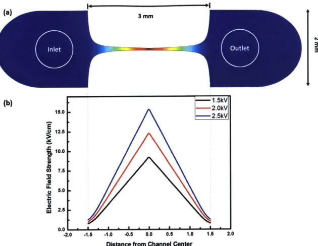
Figure 2-1 is reproduced from Figure 2 in [66], which shows the design of the mi-crofluidic assay. This assay has a bilaterally converging channel configuration, which creates a linear electric field distribution upon the application of an electric pulse. Be-fore being introduced into the channel, the cells will be mixed with SYTOX® Green nucleic acid stain (Life Technologies, Grand Island, NY), a green-fluorescent nuclear and chromosome counterstain which shows a >500-fold fluorescence enhancement upon cytoplasmic nucleic acid binding [68]. This dye is often used as an indicator of dead cells because it is impermeable to the membrane of viable cells. However, when the plasma cell membrane is compromised, the dye can penetrate the membrane and thus make the cell fluorescent even if the cell is still alive. When the electric pulse is applied and the linear electric field is established along the channel, only those cells whose membrane are no longer intact will fluoresce. Recall that only the cells that

ex-3mm (b) 15.k 15.---2.OkV 15.0 . -2.5kV E 12.5 10.0 C C 7.5 32 U. 5.0 2.5 -2.0 -1.5 -1.0 -0.5 0.0 0.5 1.0 1.5 2.0

Distance from Channel Center

Figure 2-1: Representative electric field distribution in microfluidic assay device. This microfluidic assay is designed to have a bilaterally converging channel. Section (a) shows the geometry of the microfluidic assay, which also show that the electric field strength within the 3-mm channel is amplified enough to induce electro-poration. Section (b) shows the electric field distribution within the channel when different voltage amplitudes applied across the channel (1.5kV, 2.0kV, 2.5kV), which spectrum shows that the electric field within the channel is linearly distributed. By changing the voltage amplitude, the maximum electric field strength can be controlled.

perience an electric field strength exceeding Eit will encounter membrane disruption, by identifying the transition zone along the channel where cells become fluorescent after pulse delivery within the microscope's field of view after electroporation, we can determine the location where the electric field strength reaches Eit and further calculate the corresponding electric field value. In this way, rather than repeating ex-periments with varying electric pulse amplitude, the critical electric field for inducing bacterial electroporation can be precisely quantified in a single experiment.

2.3

Determination of Critical Electric Field

[66] gives two methods to determine the position that corresponds to the critical elec-tric field, the so called "critical position". For both methods, firstly the fluorescent images are captured before and after electric pulsing. Next, the sum of the fluores-cence intensity values in the pixels perpendicular to the channel for each position along the channel for each images is calculated. After the critical position is deter-mined using two methods, the critical electric field can be easily calculated given the amplitude of applied electric pulse. Figure 2-2 and Figure 2-3 are excerpt from [661 to illustrate these two methods, respectively.

In the first method (Method I), as Figure 2-2 shows, after the sum for each position along the channel is calculated (Figure 2-2b), one-sided two-sample Kolmogorov-Smirnov (KS) test is executed at each position for calculating critical position (Figure 2-2c). KS test is a nonparametric test for comparing two groups of data based on the maximum difference between an empirical and a hypothetical cumulative distribution

[69]. One-sided two-sample KS test is specifically used for comparing whether a group of data is significantly larger than the other group. For each position along the channel, we define the two groups of data for the one-sided two-sample KS test to be the summed fluorescence intensity values for the consecutive 51 pixels near the position before and after the pulsing, respectively, where the null hypothesis Ho represents the two groups of data are drawn from a same unknown distribution. When the fluorescence intensity near the position is significantly increased after pulsing, the

null hypothesis H0 will be rejected in favor of the alternative hypothesis H1, which

represents the group of data after pulsing is significantly larger than the group of data before pulsing. By defining H value as whether Ho is accepted (H=0) or not (H=1) for each position, we can plot the H value along the channel as shown in Figure 2-2c. The position where the H value changes from 1 to 0 is the critical position, where the electric field strength is critical electric field.

Figure 2-3 shows the second method (Method II). After the sum is calculated, the empirical cumulative intensity value for each position is calculated. The empirical

cumulative intensity value is obtained by adding up all the fluorescence intensity values between that position and the position whose distance from the channel center is 1.5 mm. After subtracting the background empirical cumulative intensity value, we can clearly identify the increase of fluorescence intensity induced by electroporation by comparing the empirical cumulative intensity values before and after pulsing, and can further determine the critical position indicated with a green circle (Figure 2-3b). This method allows visual identification of the onset of electroporation-induced fluorescence enhancement.

Theoretically, the critical values determined by the two methods should be the same or be very close to each other. As for those cases where the critical values differs a lot, which are seldom scenarios, they are discussed in Chapter 4.

(a)

Before Electroporation

(b)

10

-

Before

After

E

(c)

-.

5

0

0.5

1

1.5

2

y_0.5

0

0.5

1

1.5

2

Distance from Channel Center [mm]

Figure 2-2: Method I for the determination of critical position. Section (a) shows the fluorescent images before and after delivering a 2.5-kV exponentially decaying (t = 1.0 ms; r = 5.0 ms) pulse to the trial 1 of sample 1 of Corynebacterium

glutamicum in 10% Glycerol (scale bar = 100 pm), whose experimental details are

described in Chapter 3. The yellow region is where we sum up all the fluorescence intensity values vertically. The red and blue region indicate two positions that we are interested in, and their summed data values are shown in Section (b). Section (b) and Section (c) show the summed data value and H value distribution along the channel (versus distance from the channel center). In Section (c), the position at which H changes from 1 to 0 is taken as the critical position.

CrItical Position

-(a)

E

0

(10

1.5F

IF

0.5F

0

5

0.5

1

1.5

Distance from Channel Center

[mm]

2

Figure 2-3: Method II for the determination of critical position. Section (a) shows the fluorescent images before and after delivering a 2.5-kV exponentially decaying (t = 1.0 ms; r = 5.0 ms) pulse to the trial 1 of sample 1 of Corynebacterium

glutamicum in 10% Glycerol (scale bar = 100 pm), whose experimental details are

descripted in Chapter 3. The yellow region is where we sum up all the fluorescence intensity values vertically. The red and blue region indicate two positions that we are interested in, and their summed data values after subtracting background fluorescence are shown in Section (b). Section (b) shows the back-subtracted cumulative intensity for each position before and after pulsing, where the green circle locates at the critical position.

j

Before

After

I

I

kko*'

/

-05

Chapter 3

Microfluidic Electroporation Assay

Experimental Design

3.1

Introduction

In Chapter 2, the theory and fundamental principle of the microfluidic assay was introduced. In this chapter, we use the critical electric field as a measure of cell membrane permeability to further study the effect of different buffer solutions on cell membrane permeability, and to identify the role cell polarizability plays in the process of bacterial electroporation.

We characterized the gram-positive bacteria Corynebacterium glutamicum (ATCC 13032, Manassas, VA, USA) and Bacillus subtilis 168 (ATCC 23857, Manassas, VA, USA), and the gram-negative bacteria Escherichia coli BL21 (DE3) (Bioline com-petent cells BIO-85032, London, UK) and Pseudomonas syringae ESC 10 (ATCC 55389, Manassas, VA, USA), and measured their critical electric field in 10% (v/v) glycerol and 0.01 x phosphate buffered saline (PBS) buffer (PBS diluted 100 times in DI water), respectively.

The following sections will introduce the methods used for experiments, experi-ment results, how we can interpret the experiexperi-ment results to understand the effect of different buffer solutions on cell membrane permeability, and the relationship between cell polarizability and critical electric field.

3.2

Methods

3.2.1

Culture Conditions for Bacterial Strains

Firstly, bacterial strains were all overnight-cultured in 15-mL culture tubes at 37 C.

Corynebacterium glutamicum was cultured in 5-mL brain heart infusion supplemented

with 0.5M sucrose (BHIS) medium. Bacillus subtilis 168 was cultured in 5-mL Luria broth (LB) medium. Escherichia coli BL21 (DE3) was cultured in 5-mL LB medium.

Pseudomonas syringae ESC 10 was cultured in 5-mL nutrient broth (NB) medium.

The following morning, 800 pL of cell culture was transferred to 80 mL of fresh growth media and allowed to grow to exponential phase before the electroporation

assay (OD₆₀₀ between 0.45-0.6). Then each of the strains studied were re-suspended

into 10% glycerol or 0.01 x PBS by centrifuging at 3500 rpm for one time at 4 C. Next each strain were concentrated two more times by centrifuging at 8000 rpm and re-suspended into 10% glycerol or 0.01 x PBS with a final concentration of cell at

OD600 ~~ 5 at 4 C. Immediately prior to the assay, 5 mM SYTOX® dye was added

to the cell solution for a final concentration of 5 pM in all the experiments at 4 C. The mixer of cell and dye will then be used for critical electric field measurement.

3.2.2

Electroporation Protocol and Image Data Collection

The microfluidic assay were placed within the microscope's field of view, and the mixer of cell and dye were then introduced into the microfluidic devices using syringe pump until there was visible solution at the outlet. Next, the outlet tubing was clamped with hemostats, and syringe pump was used to add more pressure in the inlet end to get rid of the bubbles remaining in the assay. After making sure the constriction region was fully filled, the platinum electrodes were connected to the

MicropulserT M Electroporator (Bio-Rad, Hercules, CA). Then the inlet tubing was

also clamped with hemostats to mitigate undesired flow, and wait for a short time until the flow is stopped. Afterwards, the green fluorescence filter (Nikon 96311 B-2E/C) in the microscope was used to take fluorescent images for data collection with a

exposure time of 300 ms. The time interval between consecutive images taken by the microscope is 300 ms, and a total of 67 images for 20 seconds were capture for each experiment trial. After starting image collections for about 7 s, a single exponentially

decaying (duration t = 1.0 ms; decay constant T= 5 ms) pulse with different voltage

amplitudes were applied for different cells.

3.3

Experiment Results

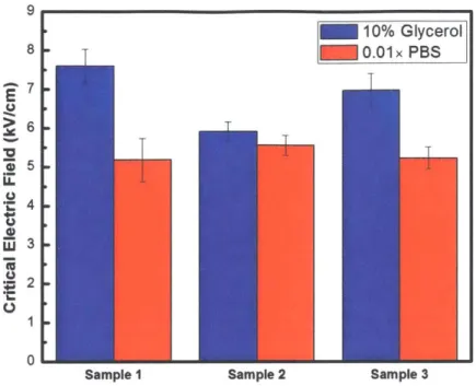
For each cell strain in each buffer solution, three biological samples were tested for determining the critical electric field. The critical electric field for each biological sample was measured for three times. Any measurement data will be discarded if and only if the image quality is too poor to be used for calculating critical electric field. Figure 3-1, Figure 3-2, Figure 3-3, and Figure 3-4 show the measured critical electric field for each cell strain in both buffer solutions, respectively. The critical electric field for each biological sample in each figure takes the average of three measurements, and the error bar represents the standard deviation of the three measurements.

U

93

M 10% Glycerol

0.Olx PBS

T

Sample I Sample 2 Sample 3

Figure 3-1: Measured critical electric field for Corynebacterium glutamicum in different buffer solutions. For sample 1 and 3, the E,. in 10% glycerol is significantly higher than E,. in 0.01x PBS. For sample 2, the E,. in two buffer solutions are almost the same.

For the sample 1 of Corynebacterium glutamicum, as the error bars in two buffer solutions don't overlap with each other, and as the average critical electric field in 10% glycerol is higher than the average critical electric field in 0.01x PBS, we can conclude that the critical electric field in 10% glycerol is higher than that in 0.01x PBS. Sample conclusion can be drawn for sample 3 of Corynebacterium glutamicum. For the sample 2 of Corynebacterium glutamicum, as the error bars in two buffer solutions overlap, we should conclude that the critical electric field in 10% glycerol is almost the same as that in 0.O1x PBS. (Figure 3-1)

Similarly, we can make conclusions for the other three strains.

10% Glycerol 0.01x PBS T 6 E5 . 3 2 *1 0 1 Sample I Sample 3

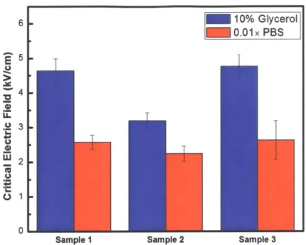
Figure 3-2: Measured critical electric field for Bacillus subtilis ent buffer solutions. For all the samples, the E,. in 10% glycerol higher than E,. in 0.01 x PBS.

168 in differ-is significantly

For any sample of Bacillus subtilis 168, the critical electric field in 10% glycerol is higher than that in 0.01 x PBS. (Figure 3-2)

T

-I-0

T

IL. 5 4 3 2 I 0

I

Figure 3-3: Measured critical electric field for Escherichia coli BL21 (DE3) in different buffer solutions. For sample 1 and 3, the E,- in 10% glycerol is significantly higher than E,. in 0.01 x PBS. For sample 2, the E,. in two buffer solutions are almost the same.

For the sample 1 or 3 of Escherichia coli BL21 (DE3), the critical electric field in 10% glycerol is higher than that in 0.01 x PBS. For the sample 2, the two critical electric field values are almost the same. (Figure 3-3)

5 10% Glycerol LZO0.01x PBS 4-3 0 OR

Sample I Sample 2 Sample 3

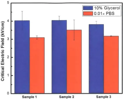
Figure 3-4: Measured critical electric field for Pseudomonas syringae in different buffer solutions. For all the samples, the Eit in 10% glycerol is almost the same as the Eit in 0.01x PBS.

For any sample of Pseudomonas syringae, the critical electric field in 10% glycerol is almost the same as that in 0.01x PBS. (Figure 3-4)

3.4

Results Analysis and Conclusions

After measuring Eit value for each sample of each strain in Figure 3-1, 3-2, 3-3, and 3-4, we will calculate the Eit value with uncertainty for each strain.

The easiest way to obtain E,, value for each strain seems to be averaging the three Eit values of three samples and using the standard deviation of three Eit values of samples as the uncertainty. However, this approach is incorrect. In this method, each measurement for each sample will contribute to the Eit equally, which makes the Eit biased a lot if one measurement is an abnormal data point. In addi-tion, notice that for each strain, the uncertainty of its E,it includes the uncertainty induced by measurement and the uncertainty induced by biology variability. The

former uncertainty is called as technical variability, which is sample-dependent and can be quantified by the standard deviation of the three measurements for each sam-ple (the error bar in Figure 3-1, 3-2, 3-3, and 3-4). The latter uncertainty, biology

variability, can be quantified by the standard deviation of three Ecit values of

sam-ples. Hence, this method actually discards the technical variability and only uses the biology variability as the uncertainty.

The right way to calculate the Ecrit value involves employing statistics knowledge.

We could regard each measurement of Erit being sampled from the Eit for a strain, so the whole measurement process corresponds to a sampling process. In such a sampling process, all the sampling (measurement) data should obey a certain but unknown distribution. If we can estimate the distribution, we can use the mean and

standard deviation of the distribution to estimate the Ecrit value and its uncertainty,

respectively. Here are the steps for determining the critical electric field for a certain strain in a certain buffer solution:

1. We assume each measurement of critical electric field for each biological sam-ple is samsam-pled from a certain but unknown distribution (this distribution will be called "unknown distribution" throughout this section), and this unknown

distribution can be inferred from the measured data;

2. We assume the unknown distribution is a normal distribution. To test this, we could use Lilliefors test to test whether the measured data comes from a distribution in the normal family. If so, we can safely assume the unknown distribution is normal distribution;

3. After confirming the unknown distribution is normal distribution, we can

esti-mate the parameters of normal distribution (mean [ and standard deviation a)

using the function "normfit()" via Matlab;

4. Use two-sided two-sample KS test to test whether measured data obeys the

normal distribution with parameters p and o-. If so, use p as the critical electric

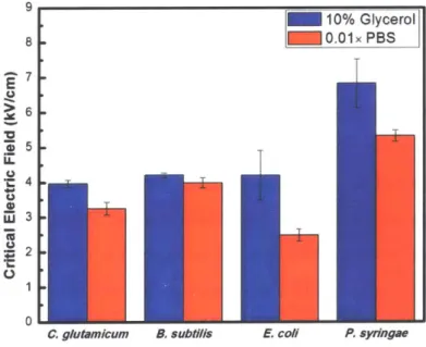
The results of applying Lilliefors test on each strain in each buffer solution (8 cases in total) show that, except the case of Escherichia coli BL21 (DE3) in 0.01 x PBS, we can assume the unknown distribution is normal distribution. The results of using the function "normplot(" via Matlab on each case are shown in Figure A-1 and Figure A-2, which function can visualize the data versus fitting normal distribution. Next, the parameters p and a for each case are calculated, and we use those parameters to obtain Figure 3-5, which shows the critical electric field for four strains in two buffer solution. Though the data points of Escherichia coli BL21 (DE3) in 0.01 x PBS don't come from a distribution in the normal family, we found that by deleting an outlier data point (the one corresponding to the largest critical electric field in the upper right subfigure in Figure A-2), the rest data points come from a normal distribution, which led us to estimate p and a for this case using the rest data points (Figure A-2).

9 10% Glycerol 8 0.01x PBS 7-E C.) >i 6 01

C. glutamicum B. subtilis E. coli P. sydingae

Figure 3-5: Measured critical electric field for different strains in different buffer solutions.

From Figure 3-5, we can conclude that for Corynebacterium glutamicum, Bacillus

subtilis 168, and Escherichia coli BL21 (DE3), the critical electric field in 10% glycerol

in 10% glycerol is almost the same as that in 0.01 x PBS.

For a certain strain, the lower its critical electric field is, the higher membrane

per-meability it has. Hence, we can conclude that 10% glycerol can make cell membrane more permeable compared to 0.01 x PBS for Corynebacterium glutamicum, Bacillus

subtilis 168, and Escherichia coli BL21 (DE3). The reason could be: (a) 10% glycerol

makes cell membrane more vulnerable due to its chemical property; (b) 10% glycerol

has a lower conductivity thus a higher electric field is needed (see the theoretical

model in Chapter 4). As a supplement for the second possible reason, we measured the conductivity of the pure buffer solution and the mixer of cell and dye (Table C. 1).

3.5

Cell Polarizability and Critical Electric Field

The theoretical model and data in this section are reproduced from an unpublished

work by Qianru Wang from the Laboratory for Energy and Microsystems Innovation

(LEMI) at MIT.

In this section, we will introduce how critical electric field correlates with cell

po-larizability based on the experiment results presented in previous sections.

Polarizability, which is a property of matter, refers to the ability to form instanta-neous dipoles when an external electric field is applied. When it comes to a cell, the

polarizability describes the ability of a cell to respond to electric fields. More

specifi-cally, the cell surface polarizability represents the overall dielectric properties at the

cell/medium interface. Recalling that in the process of electroporation an external

electric field is established, we wonder what role the cell polarizability plays during this process.

The cell polarizability here is quantified by the Clausius-Mossotti factor (KCM), a measure of the relative polarizability of the cell compared to the surrounding medium [701. The cell polarizability can be directly measured by using a microfluidic device called 3D insulator-based dielectrophoresis (3DiDEP) [701. Hence, to study how cell polarizability works in the bacterial electroporation process, we can simply measure

the cell polarizability in different conditions, e.g. different cell strains adopted or different buffer solution used, and then correlates the values of cell polarizability with markers that can represent electroporation results.

The transformation efficiency of the bacterial electroporation seems to be the best marker for such an experiment design, because this marker is usually used for eval-uating the performance of different electroporation protocols. However, considering that not only does the transformation efficiency depend on the cell property, but also replies on the property of plasmid and the uptake of plasmid, using transformation efficiency as the marker may hinder us from finding the true role the cell polarizability plays during the process of bacterial electroporation as the transformation efficiency introduces too many additional variables. Compared to transformation efficiency, the critical electric field measured by the microfluidic assay could be a much better marker, because the critical electric field only relies on the property of the cell. Hence, we finally selected the critical electric field as the marker to study the function of cell polarizability in bacterial electroporation process.

Based on the theoretical model (Appendix B), the relationship between critical electric field and cell polarizability can be written as:

TMVrit (1 - 3ArGcI)aEcritcos (3.1)

where TMVert represents the critical threshold for TMV, A is the depolarization

factor and can be expressed as A = (-_,2) (in}+e - 2e) with the eccentricity of cell

shape e

$

By utilizing the 3DiDEP device, the cell polarizability values of four bacterial strains (Corynebacterium glutamicum, Bacillus subtilis 168, Escherichia coli BL21, and Pseudomonas syringae ESC 10) in two different buffers (10% glycerol and 0.01 x PBS) were quantified (Figure A-4), and high magnification microscopy was used to measure the cell morphological parameters (Figure A-5). Together with the measured critical electric field measured in previous sections, now we could verify the correctness of the model above.

' C. glutamicum in 10% Glycerol \ C. glutamicum in 0.01 x PBS

8 \ * B. subtilis in 10% Glycerol * B. subti/s in 0.01 x PBS

A E. coiBL21 (DE3) in 10% Glycerol

E

Figure 3-6: Correlation between critical electric field and cell polarizability.

Curve fitting of data suggests that for four bacterial strains in different buffer

solu-tions, their critical TMV values are roughly 0.6 V with a goodness of fitting R 2=0..75.

This figure is reproduced from

Qianru

In Figure 3-6, Ec,. versus (1 - 3Ancm)a is plotted, where the dash-dot curve is

fitted using a power law. The fitting result shows that pore formation is induced in the four types of bacteria when their TMV reaches a constant value of roughly 0.6 V. This relationship between cell polarizability and critical electric field gives us another point of view to understand the critical electric difference across different strains and different buffers: when different strains or different buffer solutions are used, their polarizabilities change, which lead to the change of critical electric field values. Specifically, for a certain strain, as the cell polarizability in 10% glycerol is higher than that in 0.01 x PBS (Figure A-4), the corresponding critical electric field is lower (Figure 3-5).

Chapter 4

Analysis of Undesired Phenomenon

during Electric Field Measurements

4.1

Introduction

Given the explicit principle of the microfluidic assay introduced in Chapter 2 and the detailed experiment protocols stated in Chapters 2 and 3, the results analysis in Chapter 3 seems to be sufficient. However, there are still some unexpected phenomena that would probably affect the experiment results. Hence, in this chapter, we will discuss those phenomena, and identify or even quantify how they will influence the experiment results.

4.2

Electroosmosis and Electrophoresis

When electric field is applied across a fluid conduit, e.g. porous material, capillary tube, and membrane, the fluid as well as the particles dispersed in the fluid will move. The motion of the fluid and the motion of the particles relative to the fluid are called electroosmosis and electrophoresis, respectively.

In this work, both phenomena occurred during the pulsing time. Though the pressure of the inlet and outlet were balanced by using tubing clamps and waiting until flow subsided before applying the electric pulse, when the electric pulse was applied,

the cells still moved towards anode, as shown in Figure 4-1. During the pulsing time,

the total velocity of the cells vcelI was the sum of the velocity of electroosmosis and the

velocity of electrophoresis, which can be written as v, 11 = velectroosmosis+Velectrophoresis.

Hence, the distance shift of cells uc1 during and after the pulse can be written as

Ucell = Uelectroosmosis + Uelectrophoresis. Since the cells in the channel were exposed to

a continuous electric field spectrum, this distance shift led to a critical electric field shift during measurement. This critical electric field shift during and after the pulse,

which was recognized as AEit in

166],

of a single fluorescent bacterium at the transition zone and correlating the distance traveled by this bacterium from the last pre-pulse to the first post-pulse image to the corresponding shift in local electric field experienced by that bacterium.

In order to achieve a more precise measurement of critical electric field, we need to mitigate AEit, thus it is necessary to study what factors would affect AEit and how they affect AEit. Here we propose a model for deriving the expression for

AEcrit.

As the pulsing time is 1 ms, which is relatively short, we can still regard the

distance shift ucell is too small to cause a pressure difference between inlet and outlet.

Hence, the expression u,1j = Uelectroosmosis + Uelcctrophoresis is still valid. As both the

velocity of electroosmosis and the velocity of electrophoretic is proportional to the electric field, the velocity of the cells is also proportional to the electric field, which further leads to the distance shift of the cells proportional to the electric field:

Uceii(x) oc E(x) (4.1)

where the x represents the position of the cell studied, which is defined as the distance

from the channel center along the channel, and ucc1(x) and E(x) are the distance shift

of the cell and the electric field strength in the position x, respectively. Note that the

relationship between AErit and uce11(x) is:

Figure 4-1: Cell shift caused by electroosmosis and electrophoresis. Fluores-cent images (a) before and (b) after delivering a 1.5-kV exponentially decaying (t =

1.0 ms; -r = 5.0 ms) pulse to the trial 2 of sample 3 of Bacillus subtilis 168 in 0.01 x

PBS (scale bar = 100 am). The center of channel is indicated in blue, the shift of the cell 1 is indicated in red, and the shift of the cell 2 is indicated in green. We can find that the closer to the channel center a cell is, the larger shift it has. The red (green) dash-dot lines indicate the shift distance for cell 1 (cell 2).

where the xeit is the position corresponding to the transition zone, where E(xcrit) =

E,.it. Hence, we have:

A Ec,.it oc VxE,(xe,.t| = Ecit -IVxE(x,.)tI (4.3)

For a specific cell strain, the Eit is only determined by the cell property, hence we can regard it as a constant in above formula, which finally lead to:

Hence, we need to minimize

IVE(xzet)

From Figure 2-1, we can easily know that

IVxE(zrt)

amplitude of electric pulse, and that given an amplitude of applied electric pulse, the jVxE(xze)j, which represents the gradient of electric field along the channel, is linearly distributed inside the whole channel, despite a slight decrease near the

boundary of the channel. So the final answer for minimizing AEcr now seems to

be using the lowest amplitude for pulsing. This can be verified by the data in [661, where for each strain, the average AEct will increase as the amplitude of applied pulse increases.

However, when a pulse with small amplitude is applied, the transition zone will be near to the channel center, thus other undesired phenomena would harm the accuracy of critical electric field. For example, when the transition zone is near to the channel center, we would have few cells fluorescent after pulsing compared to the total volume of cells in the whole channel, which would lead to poor image quality; when there is flow caused by other undesired phenomena, e.g. caused by pressure gradient, the shift near the channel center will be significant since the region near channel center is narrow, and thus the error of critical electric field caused by this shift will be relatively large. So we need to trade-off those effects for selecting an optimal amplitude of applied electric pulse.

In all the experiment trials in Chapter 3, the maximum AEcr is 0.12 kV/cm. Compared to the value of a in each case, where the smallest a is 0.3247 kV/cm, this

AEcrit is not significant. This comparison suggests that the electric pulse amplitude values we selected for experiment were proper.

4.3

Contradiction between Methods for Critical

Elec-tric Field Determination

In Chapter 2, we presented two different methods for determining critical electric field

electric field value. However, in some situations, the critical electric field values calculated by the two methods are different. This section aims at analyzing the reason behind this phenomenon.

Figure 4-2 is an example of this situation, which shows the transition zone

posi-tion xzit of trial 1 of sample 3 of Bacillus subtilis 168 in 0.01 x PBS measured by

two methods. The left subfigure shows that, when using Method I, the position of

transition zone xzit = argmaxH(x) =1.221 mm. The right subfigure shows that,

when using Method II, the transition zone, which is the crossover point of two curves,

is Point B xit =0.936 mm. As the xxit determined by the two methods are different,

the corresponding critical electric field quantified by two methods will be different.

K-S test result X 105 Back-subtracted cumulative data

2_{r 1 ---- - - ___ _ _}

Before

After

3-C

1 _{Point A Point B Point C} 0"

-6.5 0 0.5 1 1.5 2 -1 -0.5 0 0.5 1 1.5 2

x [mm] x [mm]

Figure 4-2: Using Method I and Method II to determine the critical electric field. This figure shows using Method I (left) and Method II (right) to determine the xit for further calculating the critical electric field of the trial 1 of sample 3 of

Bacillus subtilis 168 in 0.01x PBS.

To find the reason for the contradiction, it is necessary to plot the fluorescence intensity in each position along the channel. Figure 4-3 shows the fluorescence inten-sity before and after the pulse along the channel. On the blue curve in Figure 4-3, there are three local minimum points (Point 1, Point 2, and Point 3), which lead to the three local minimum points on the blue curve in the right subfigure of Figure 4-2. These local minimum points deform the blue curve, which finally result in the change of the intersection point.

1.

0.

Box averaging only

150

Before

After

100-*

50-

Point 2

<CD

tPoint

₃

Point 1

-501

1

-0.5

0

0.5

1

1.5

2

x [mm]

Figure 4-3: Fluorescence intensity before and after the pulse along the chan-nel. This is the trial 1 of sample 3 of Bacillus subtilis 168 in 0.01 x PBS.

The three local minimum points come from the flow in the channel when the electric pulse applied, which flow may be caused by electroosmosis, electrophoresis, or other undesired phenomena such as pressure gradient. Figure 4-4 shows the fluo-rescence images before and after the pulse. In Figure 4-4, each local minimum point (Point 1, Point 2, and Point 3) has a big cluster of fluorescent cells in the image before pulse. After applying the pulse, those clusters of cells move leftward, which makes the fluorescence intensity in previous positions lower. When the fluorescence intensity in a, certain position is lower after the pulse, there will occur a local minimum point.

Figure 4-4: Clusters of cells moving leftward. Fluorescent images (a) before and

(b) after delivering a 1.5-kV exponentially decaying (t = 1.0 ms; T = 5.0 ms) pulse

to the trial 1 of sample 3 of Bacillus subtilis 168 in 0.01 x PBS (scale bar = 100 pm). The center of channel is indicated in blue, and the three clusters of cells moving leftward are indicted in red (Point 1), green (Point 2), and orange (Point 3).

After know the reason of the contradiction, we now can know that the x,t

ob-tained by using Method I is still correct, so we can calculate critical electric field using

this x,.t. In addition, as those cluster of cells are the dead cells, which will be lighted

up before the pulse, we know that by reducing the number of dead cells introducing into the channel, we can mitigate this phenomenon.

Chapter 5

Conclusions and Future Work

In this work, we used microfluidic assay to quantify the critical electric field of

differ-ent cell strains (Corynebacterium glutamicum, Bacillus subtilis 168, Escherichia coli BL21 (DE3), and Pseudomonas syringae ESC 10) in different buffer solutions (10%

glycerol and 0.01 x PBS). Experiment results reveal that, for Corynebacterium

glu-tamicum, Bacillus subtilis 168, and Escherichia coli BL21 (DE3), the critical electric

field values in 10% glycerol are higher than that in 0.01 x PBS, which indicates that using 10% glycerol as the buffer solution for bacterial electroporation can me the cell

membrane more permeable compared to using 0.01x PBS. We investigated the cor-relation between cell polarizability and critical electric field. In addition, we analyzed

undesired phenomena during the experiments, e.g. cell shift caused by electroosmosis

and electrophoresis, and explored how those phenomena would affect the accuracy of the measured critical electric field.

However, there are still opportunities for future work on the improvement of the

accuracy of this microfluidic assay. As the electrodes inserting into the inlet and

outlet will scatter and reflect the fluorescent light during the experiment, which will

generate fluorescence noise in the image so that the accuracy of measured critical

electric field will decrease, it is necessary to develop a better design on the geometry

of assay inlet and outlet. It is also meaningful to have a graduation besides the

channel indicating the electric field strength in the channel, which could enable us to

This assay can also be used for more applications. The critical electric field of more types of cell strain can be can be quantified to study how cell membrane features contribute to the electroporation process. By using new dyes/molecules rather than SYTOX, or by using ncw buffer solutions, we can explore how the permeability of the cell membrane changes in different conditions.