Convex relaxation methods for graphical models : Lagrangian and maximum entropy approaches

(1)

Convex Relaxation Methods for Graphical Models:

Lagrangian and Maximum Entropy Approaches

by

Jason K. Johnson

Submitted to the Department of Electrical Engineering and Computer Science in partial fulfillment of the requirements for the degree of

Doctor of Philosophy in

Electrical Engineering and Computer Science at the Massachusetts Institute of Technology

September, 2008

Signature of Author:

Dipartment of Electri 1 Engineering and Computer Science August 18, 2008

Certified by:

Alan S. Willsky, Professor of EECS Thesis Supervisor

Accepted by:

Terrys. Orlando, Professor of Electrical Engineering Chair, Department Committee on Graduate Students

IOCT 2 2 2WA

LIBRARIES

(2)

(3)

--Convex Relaxation Methods for Graphical Models:

Lagrangian and Maximum Entropy Approaches

by Jason K. Johnson

Submitted to the Department of Electrical Engineering and Computer Science on August 18, 2008

in Partial Fulfillment of the Requirements for the Degree

of Doctor of Philosophy in Electrical Engineering and Computer Science

Abstract

Graphical models provide compact representations of complex probability distribu-tions of many random variables through a collection of potential funcdistribu-tions defined on small subsets of these variables. This representation is defined with respect to a graph in which nodes represent random variables and edges represent the interactions among those random variables. Graphical models provide a powerful and flexible approach to many problems in science and engineering, but also present serious challenges owing to the intractability of optimal inference and estimation over general graphs. In this thesis, we consider convex optimization methods to address two central problems that commonly arise for graphical models.

First, we consider the problem of determining the most probable configuration-also known as the maximum a posteriori (MAP) estimate-of all variables in a graphical model, conditioned on (possibly noisy) measurements of some variables. This general problem is intractable, so we consider a Lagrangian relaxation (LR) approach to obtain a tractable dual problem. This involves using the Lagrangian decomposition technique to break up an intractable graph into tractable subgraphs, such as small "blocks" of nodes, embedded trees or thin subgraphs. We develop a distributed, iterative algo-rithm that minimizes the Lagrangian dual function by block coordinate descent. This results in an iterative marginal-matching procedure that enforces consistency among the subgraphs using an adaptation of the well-known iterative scaling algorithm. This approach is developed both for discrete variable and Gaussian graphical models. In dis-crete models, we also introduce a deterministic annealing procedure, which introduces a temperature parameter to define a smoothed dual function and then gradually reduces the temperature to recover the (non-differentiable) Lagrangian dual. When strong du-ality holds, we recover the optimal MAP estimate. We show that this occurs for a broad class of "convex decomposable" Gaussian graphical models, which generalizes the "pairwise normalizable" condition known to be important for iterative estimation in Gaussian models. In certain "frustrated" discrete models a duality gap can occur using simple versions of our approach. We consider methods that adaptively enhance the dual formulation, by including more complex subgraphs, so as to reduce the duality gap. In many cases we are able to eliminate the duality gap and obtain the optimal MAP estimate in a tractable manner. We also propose a heuristic method to obtain approximate solutions in cases where there is a duality gap.

(4)

and its potential functions) from sample data. We propose the maximum entropy relaxation (MER) method, which is the convex optimization problem of selecting the least informative (maximum entropy) model over an exponential family of graphical models subject to constraints that small subsets of variables should have marginal distributions that are close to the distribution of sample data. We use relative entropy to measure the divergence between marginal probability distributions. We find that MER leads naturally to selection of sparse graphical models. To identify this sparse graph efficiently, we use a "bootstrap" method that constructs the MER solution by solving a sequence of tractable subproblems defined over thin graphs, including new edges at each step to correct for large marginal divergences that violate the MER constraint. The MER problem on each of these subgraphs is efficiently solved using the primal-dual interior point method (implemented so as to take advantage of efficient inference methods for thin graphical models). We also consider a dual formulation of MER that minimizes a convex function of the potentials of the graphical model. This MER dual problem can be interpreted as a robust version of maximum-likelihood parameter estimation, where the MER constraints specify the uncertainty in the sufficient statistics of the model. This also corresponds to a regularized maximum-likelihood approach, in which an information-geometric regularization term favors selection of sparse potential representations. We develop a relaxed version of the iterative scaling method to solve this MER dual problem.

Thesis Supervisor: Alan S. Willsky

(5)

Acknowledgments

I thank my thesis advisor, Alan Willsky, for accepting me into his group and for guiding and supporting my research over the years. As his student, I have enjoyed an uncommon level of intellectual freedom that has allowed me to explore a wide range of ideas. I have great respect for his integrity, dedication and enthusiasm. I am also grateful for his meticulous reading of the thesis and for his rapid return of drafts. I thank my thesis committee members, Sanjoy Mitter and Tommi Jaakkola, for their advice and for quickly reading a draft of the thesis.

I thank Bob Washburn, Bill Irving and Mark Luettgen, whom I worked with at Alphatech, Inc. (now the AIT Division of BAE systems), for having inspired me to pursue a graduate degree in electrical engineering and computer science. I am grateful to all of my past "grouplet" members for the influence they have had on my research: Mike Schneider, Dewey Tucker, Martin Wainwright, Erik Sudderth, Dmitry Malioutov, Venkat Chandrasekaran, Jin Choi, Lei Chen, Pat Kreidel and Ayres Fan. In particular, I thank Dmitry and Venkat for their collaboration on numerous research topics, including work presented in this thesis. I have especially enjoyed our Wednesday night treks, often joined by Pat and Ayres, to the Muddy Charles for drinks over a game of cards. Also, I thank Evan Fortunato and Mark Luettgen for bringing me back to Alphatech one summer to work on multi-target tracking, which sparked some ideas that led to the Lagrangian relaxation work presented in this thesis.

I thank my parents for pretty much everything, particularly for having always en-couraged me to go my own way in life. I thank Joel Gwynn for being a good friend and for providing no-nonsense advice when I needed it. I also thank Tricia Joubert for being my best friend and companion these past four yours. She has been an essential support as I have dealt with the stresses of completing the doctoral program.

(6)

(7)

Chapter 1 Introduction

U 1.1 Motivation and Overview

Graphical models [43, 60,145,185] are probabilistic models for complex systems of ran-dom variables where the joint probability distribution of all variables is compactly specified by a set of interactions among variables. In the case of undirected graphical models, which we also refer to as Markov random fields (MRFs), each interaction is specified by a potential function, defined on a subset of the variables, that provides a relative measure of compatibility between the different joint configurations of these vari-ables. The structure of the model thus defines a graph, each variable is identified with a node of the graph and interactions between variables define edges of the graph. In some cases, the probability model actually represents some naturally occurring random process. In others, we seek to optimize some objective function, which may be then be interpreted as finding the ground state of the Gibbs distribution [90] based on this objective function. Models of this form arise in many fields of science and engineering:

* statistical physics [129,195,229], * signal processing [16,19,83,130,207], * image processing [28,88,149,222,223],

* medical imaging and tomography [84, 176], * geophysics and remote sensing [55, 112,126,197], * circuit layout design [12, 148, 151],

* communication and coding theory [85,153,179], and

* distributed estimation in sensor networks [44,51,66,113,162, 189,224].

However, the utility of these models in practical applications is often limited by the fact that optimal inference and optimization within this model class is generally in-tractable for large problems with many variables [10, 58]. As a result, there has been an intense, ongoing effort in recent years to develop tractable yet principled approaches to approximate inference within this rich class of models.

(12)

In this thesis, we focus on two central problems that arise for graphical models. First, we consider the problem of maximum a posteriori (MAP) estimation. That is, given a graphical model defined on a set of variables, and possibly partial observa-tions (e.g., noisy measurements) of subsets of these variables, we seek a joint estimate of all unknown variables that maximizes the conditional joint probability of the esti-mate given the observations. In general, this problem is NP-hard to solve exactly in models with discrete (e.g., binary valued) variables. We develop a Lagrangian relax-ation (LR) method [22,80,89] that decomposes the problem into tractable subproblems defined on smaller or more tractable subgraphs. This general approach of splitting an intractable problem into tractable subproblems, by introducing copies of some variables and relaxing equality constraints between these copies, is also known as Lagrangian de-composition [48,100, 159] (we use these terms interchangeably in this thesis). In many cases our graphical decomposition approach leads to the optimal MAP estimate, in which case one says that strong duality holds. However, because the general problem is NP-hard, we must expect to also encounter cases where there is a a duality gap and the optimal MAP estimate cannot be obtained. We also propose a simple heuristic method to obtain approximate solutions in this case.

The second problem we consider is that of model selection [41,106], that is, of select-ing both the graph structure and a correspondselect-ing set of potential functions to obtain a good fit to sample data. Our approach to this problem of learning a graphical model from sample data is also useful if one instead seeks to thin a graphical model, that is, to adaptively select a simpler graphical model that still provides a good approximation to a more complex model. While early work on these problems has focused on primarily on greedy combinatorial approaches to select the graph structure [67, 177,199], we fo-cus instead on a convex optimization approach to simultaneously learn both the graph and its potentials. The main idea is to relax the well-known maximum entropy mod-eling approach [59, 97, 117, 177] to obtain a regularized maximum entropy method, one that implicitly favors sparser graphical models. This involves introducing constraints on the marginal distributions of the model, that they should be close to the empirical marginals (from sample data or a more complex model that we wish to thin) as mea-sured by relative entropy [59] (also known as Kullback-Leibler divergence [142,143]). We also derive a dual version of this problem which leads naturally to a relaxed versions of the iterative scaling algorithm [62, 114, 186, 199], often used for learning graphical models with a fixed graph structure.

A key idea common to both of these approaches is seeking convex relaxations of intractable problems [37]. In the case of Lagrangian relaxation for discrete graphical models, a non-convex integer programming problem is relaxed to the convex Lagrangian dual problem. In maximum entropy relaxation, the non-convex problem of selecting a graph is relaxed to convex optimization over a denser graph (e.g., the complete graph) but with a regularization method to enforce sparsity in the potentials on this denser graph, thereby selecting a sparse subgraph.

(13)

Sec. 1.2. Related Work

* 1.2 Related

Work

Before discussing our methods and contributions further, we give a brief account of relevant work on tractable inference and learning methods for graphical models and of approximate methods for intractable models. A more detailed discussion of many of these approaches is given in the background (see Chapter 2).

* 1.2.1 MAP Estimation

Dynamic Programming and Combinatorial Optimization

There are several classes of graphical models for which inference is tractable, either to compute the marginal distributions of individual variables or the MAP estimate. In graphs with low tree-width [6, 31,32], one can exactly compute either marginals or the so-called max-marginals to obtain the MAP estimate. These approaches involve variable elimination steps that either sum or maximize over individual variables to obtain marginals. In the case of maximizing (to solve the MAP problem), this method is a generalization of well-known dynamic programming methods such as the Viterbi algorithm [16, 19, 83,207]. In order to apply this tree-structured inference procedure to general graphs, one converts the graph to a tree using the concept of junction trees [146]. Roughly speaking, this involves grouping nodes together to define an equivalent Markov tree representation of the model. The tree-width is determined by how many nodes must be grouped together in this procedure. In the class of bounded tree-widths graphs, the computational complexity of this procedure grows linearly in the number of nodes. However, its complexity is exponential in the tree-width and it is therefore only tractable for thin graphs, that is, for graphs with low tree-width.

However, for special classes or problems it is still possible to solve the MAP prob-lem exactly even if the graph is not thin. We mention only a few well-known exam-ples. First, there are a number of well-studied combinatorial and network optimization problems that have efficient solutions [42,171], including: the max-cut/min-flow prob-lem [82], maximum-weight matching in bipartite graphs [73], and minimum-weight per-fect matching in planar graphs [57, 165]. Several connections have been found between such network optimization problems and MAP estimation in graphical models. For example, the ferromagnetic Ising model can be solved exactly using a max-flow/min-cut reformulation of the problem [11, 98]. This is a binary variable graphical model, with node states +1 and -1, in which all interactions are pairwise and where the pair-wise potentials prefer configurations in which adjacent variables are assigned the same value. Similarly, zero-field Ising models defined on planar graphs can be solved exactly as a minimum-weight perfect matching problem [29, 87, 172,203]. In this case, pairwise potentials may also be anti-ferromagnetic so as to prefer configurations in which ad-jacent nodes have opposite states. But the model is required to have zero-field, which essentially means that every configuration and its negation (with all nodes assigned opposite values) are equally likely. MAP estimation in the general Ising model can be reformulated as a max-cut problem [12, 13]. Although it is not tractable to solve

(14)

max-cut in general graphs, Barahona and Mahjoub have proposed a heuristic cutting-plane method based on the odd cycle inequalities [13]. In planar graphs, this leads to an optimal solution of the max-cut problem and therefore solves the zero-field planar Ising model. Other connections to network optimization have emerged. For instance, a number of works have recently appeared using linear-programming relaxations of the MAP estimation problem [50, 76, 133, 211, 219]. In earlier work on binary quadratic programming [34,36,103], it was found that the value of this linear program (LP) can be computed using max-flow/min-cut techniques. In cases where solution of the LP leads to an integral solution, the correct MAP estimate is obtained. Otherwise, there is an integrality gap and the value of the LP provides an upper-bound on the value of the MAP problem. Other approaches use LP methods in conjunction with the branch and bound procedure, and often succeed in identifying the MAP estimate [196]. How-ever, the number of steps required to reach an optimal solution may be exponential in problem size in the worst-case.

Many methods have appeared in the graphical modeling literature aimed at solv-ing (at least approximately) the MAP estimation problem. This problem is closely related to that of computing marginal distributions of the model. The sum-product

algorithm [85], also known as belief propagation (BP) [175], is an iterative message-passing algorithm for computing approximate marginal distributions of each variable in a graphical model. It is based on an exact inference method for trees, which in-volves passing messages along the edges of the tree. Each node fuses messages, from all but one its neighbors, and then propagates this information to the excluded neighbor based on the edge potential linking the two nodes. In loopy graphs, this procedure does not always converge to a fixed-point and may give inaccurate marginals when it does converge. Nonetheless, it has yielded good results in many practical applications. Another form of belief propagation, the max-product algorithm, may be regarded as approximating the "zero-temperature" marginals of a graphical model, which encode the distribution of a variable over the set of MAP estimates, and is closely related to dynamic programming methods such as the Viterbi algorithm. Convergence of max-product tends to be less robust than the sum-max-product algorithm. Also, if max-max-product does converge it may still give an incorrect MAP estimate. However, this estimate does at least satisfy a certain local-optimality condition with respect to induced subtrees of the graph [218].

More recent work has focused on convex forms of belief propagation [219,226], start-ing with the work of Martin Wainwright [211,212] on approximation methods based on convex decompositions of a graphical model into a set of more tractable models defined on spanning trees (see also earlier work on fractional belief propagation [221]). Max-product forms of these methods, such as tree-reweighted max-Max-product (TRMP) [211], aim to minimize a convex function that is an upper-bound on the MAP value. This cor-responds to a linear-programming dual [25] of previously considered LP relaxations of MAP estimation, either based on an outer-bound approximation of the marginal poly-tope [50,133] or the standard linearization method [216] (see also [103]). The advantage

(15)

of such dual methods is that they provide efficient solution methods based on BP-like distributed message-passing algorithms (see [226] for an empirical comparison between message-passing approaches and traditional approaches to solve linear programs). How-ever, because belief propagation does not always converge, there is growing interest in other convergent iterative methods to solve these dual formulations using coordinate-descent methods. This includes our own work presented in this thesis and in our earlier paper [125], based on the Lagrangian decomposition formulation, as well as other recent work [93,134] that also used coordinate-descent approaches. Also, Tom Werner recently published a paper [220] reviewing earlier work [140, 192], not previously published in English, on the max-sum diffusion algorithm. All of these methods lead to similar style update rules but are not precisely equivalent because they use different param-eterizations such that coordinate-descent in these different parameterization does not lead to equivalent algorithms. One difficulty encountered in such coordinate-descent approaches, when applied to a non-differentiable objective (such as the dual functions that arise in these formulations), may get stuck at a non-minimum fixed point of the algorithm [134, 191]. One proposal to address this problem has been to use instead a low-temperature version of the convex sum-product algorithm [219]. Although this approach is very reasonable insofar as it "smoothes" the objective function, the issue of convergence (and rate of convergence) of this algorithmic approach has not been resolved. For instance, it is known that even convex versions of BP do not necessarily converge. Using sufficient damping of message updates may help, but it seems unlikely to be very efficient at low temperatures. Our approach uses a temperature anneal-ing idea to overcome this difficulty in conjunction with a coordinate-descent method. However, our approach is deterministic, and should not be confused with randomized algorithms such as simulated annealing [88]. In this regard, our approach is in the same spirit as several methods developed in the neural network literature for solving combinatorial optimization problems [95,139,178].

While this thesis was in preparation, several other papers have appeared, in ad-dition to our publication [125], that independently propose Lagrangian decomposition approaches to MAP estimation in graphical models [137,230]. Also, we recently dis-covered earlier work of Storvik and Dahl on this topic [200]. All of these methods only consider decompositions that are equivalent to the simplest pairwise relaxation in our method.1 Also, all of these papers minimize the dual function using subgradient meth-ods, a standard approach from the integer programming literature, which often suffers from slow convergence to the minimum of the dual function (in the worst case, the rate of convergence is sublinear).

Gaussian Inference

We are also interested in the problem of MAP estimation in large-scale Gaussian graph-ical models, also known as Gauss-Markov random fields (GMRFs) [144, 185, 199]. For

1

Although [200] considers a decomposition of a 2D grid in vertical and horizontal chains, this is actually equivalent to the pairwise relaxation.

(16)

GMRF models, MAP estimation reduces to minimizing a convex, quadratic objective function based on a sparse, symmetric positive-definite matrix, the information ma-trix of the model. Equivalently, the optimal solution of this minimization problem can be obtained by solving a linear system of equations based on the information matrix. This solution can be computed directly by Gaussian elimination [96], which has cubic computational complexity in the general case. For GMRFs, the graphical structure of the model is determined by the fill-pattern (sparsity) of the information matrix. This enables solution methods using sparse elimination procedures, such as the nested dissection procedure for computing a sparse Cholesky factorization of the information matrix, which results in computational complexity that is cubic in the tree-width of the graph (rather than the total number of variables) [182,185]. While this is a tremendous improvement for sufficiently thin models, it is still unsatisfactory for many applications where Gauss-Markov random fields occur with very large tree-width, such as in 2-D models commonly used for image processing and remote sensing (where tree-widths of

1,000 or more are common) or in 3-D models used for tomography or remote sensing (where tree-widths of 100 x 100 = 10, 000 are common). In such applications, it is im-practical to use direct factorization methods and it becomes preferable instead to use iterative methods that obtain approximate solutions with computational complexity (per iteration) that scales linearly in problem size. For instance, one might use classical iterative methods such as the Gauss-Jacobi or Gauss-Seidel iterations [206]. The em-bedded trees algorithm [201] and its variants [45,47,66] were developed to accelerate the convergence of iterative methods. These are iterative methods that use a sequence of preconditioners, based on embedded trees or other tractable subgraphs, to update the estimate based on the residual error at each iteration.

Another approach is to use the Gaussian form of belief propagation [124,157, 217]. It has been shown [217] that if Gaussian BP converges then it recovers the correct MAP estimate, which, for GMRFs, is equivalent to computing the mean value of each variable. In addition to computing these means, Gaussian belief propagation also com-putes approximate variances of each variable. Recent work on the walk-sum view of inference in Gaussian graphical models [47, 124, 157] has shown that a wide range of iterative methods may be viewed as computing sums and, for the class of walk-summable models, these iterative methods are guaranteed to converge to the correct MAP estimate. In other work, a recursive divide and conquer approach to approxi-mate inference in GMRFs has been proposed using a combination of nested dissection, Gaussian elimination and model thinning operations [118,126]. This approach leads to improved variance estimates and rapid convergence to the correct means when used as a preconditioner. Another method for computing approximate variances was developed in [155,156]. This approach relies upon fast linear solvers and a low-rank approximation to the identity matrix. Then, the covariance matrix, which is equal to the inverse of the information matrix, is approximated by solving a small number of linear systems.

(17)

* 1.2.2 Learning Graphical Models

Parameter Fitting

For a fixed graph structure, learning a graphical model involves selecting the potential functions of the model to obtain the best fit of the overall probability distribution to observed sample data of the model variables. The standard method is to maximize the likelihood of the sample data as a function of the model parameters [81, 174], which specify the potential representation of the graphical model. If there are no hidden variables, that is, if the sample data consists of complete observations of all variables in the graphical model, then this may be posed as a convex optimization problem in an exponential family model (e.g., the Gibbs representation of a discrete variable model) and solved using standard convex optimization methods [24, 37]. However, computing the likelihood, or its gradient, is just as as difficult as inference, that is, computing marginal distributions of the model. For this reason, maximum-likelihood modeling is only tractable for models for which exact inference is tractable. Otherwise, one must resort to approximate learning, based on approximate inference or Monte-Carlo methods to estimate marginal distributions of the model.

The iterative scaling algorithm, also known as iterative proportional fitting, is one common approach to learning graphical models [62,114,186,199]. This procedure iter-atively adjusts the potentials of the graphical model by multiplying each potential (in the product representation of the graphical model) by the ratio of the empirical dis-tribution of the corresponding variables (obtained from sample data) divided by their marginal distribution in the current estimate of the model (computing by some inference method). This has a geometric interpretation, within the information geometric view of the exponential family, as computing the minimum relative-entropy projection onto the set of models that are consistent with the data. The iterative scaling procedure performs a sequence of such projections, where each projection imposes consistency with the data for a subset of nodes. By iterating over all subsets of interacting nodes, this sequence of projections converges to the desired projection onto the intersection of the feasible sets of all constraint.

This approach can be extended to learn hidden-variable models, where not all vari-able of the model are observed. If there are hidden varivari-ables, then the maximum-likelihood problem generally becomes non-convex and may exhibit multiple local min-ima. The expectation-maximization algorithm [68] is an iterative two-step procedure. At each iteration of the algorithm: (1) The E-step determines a concave lower-bound of the log-likelihood function that is tight for the current model estimate. This involves inference calculations to compute marginal distributions of hidden variables and their coupling to adjacent variables. (2) The M-step maximizes this lower-bound to obtain the next set of model parameters. This procedure is then repeated for this new set of model parameters and continues until a fixed point of the algorithm is reached. This method is guaranteed to monotonically increase the log-likelihood and to converge to a local maximum. The maximization step can be solved using the same inference and

(18)

convex optimization methods as are used to solve the maximum-likelihood problem when there are no hidden variables.

Structure Learning

Often, we may not know the correct graph structure to use for modeling some collection of random variables. Then, it is natural to seek a good graph structure based on sample data. Here, one is faced with the problem of over-fitting. That is, if we allow a very complex graph (with many edges and associated potential functions), this tends to over-fit the sample data, leading to poor generalization performance when we compare the learned model to new sample data. Thus, one must find ways to regularize the model selection to penalize overly complex models. Another concern is that denser graphical models tend to be less tractable for inference calculations, providing further motivation for seeking less complex graphs.

One approach is to add a penalty term to the maximum log-likelihood objec-tive which explicitly favors low-parameter models, as in the Akaike information cri-teria [2, 174] which uses the to-norm of the parameter vector as a measure of model complexity. In the Gibbs representation of a graphical model, where the model pa-rameters correspond to interactions between variables, this is essentially equivalent to favoring sparse graphs. However, the eo-regularized problem is non-convex and generally intractable to solve for large numbers of variables. Nonetheless, a number of incremen-tal greedy feature selection methods have been developed which aim to approximately solve this model selection problem [64,67,69,199].

Another approach is instead to restrict oneself to some specified set of low-complexity graphs. This approach is also combinatorial in nature and cannot generally be solved exactly by a tractable method. One exception, however, is the case of finding the best tree. This can be formulated as a maximum-weight spanning tree problem that can be solved exactly using a greedy method [56]. Unfortunately, the generalization to finding maximum-likelihood bounded tree-width graphs is NP-complete and one must again resort to approximation methods [131].

Recently, several methods have appeared that use f-regularization to favor sparser1

graphical models [9,147,214]. This may be viewed as a convex proxy for lo-regularization. A dual interpretation of such methods is provided by the regularized maximum entropy method [72]. In particular, fl-regularized maximum-likelihood is the dual problem associated with finding the maximum entropy distribution over the set of probabil-ity distributions where the expected values of the sufficient statistics of the model are close to the sample average in the

4o

distance metric. This may also be viewed as robust maximum-likelihood estimation [9], which allows for uncertainty of the empirical moments. It is noteworthy that relaxing the parameter estimation in this way auto-matically leads to selection of sparse graphical models obtained by solving a convex optimization problem. This is also a critical feature in our approach.

(19)

Sec. 1.3. Contributions

* 1.3 Contributions

E

1.3.1 Lagrangian Relaxation for MAP Estimation

We develop a general Lagrangian relaxation (LR) approach to MAP estimation based on the idea of decomposing an intractable graphical model into a collection of tractable sub-models (e.g., defined on small subgraphs or on thin subgraphs such as trees), and study the conditions for strong duality to hold in this relaxation. For discrete variable models, we develop an algorithmic approach for solving the resulting dual problem based of a finite-temperature smoothing technique (using a deterministic annealing procedure to gradually reduce the temperature) and the iterative scaling algorithm to minimize a smoothed version of the dual function at each temperature. Additionally, we develop heuristic methods to either (i) enhance the relaxation to include additional structure so as to reduce or eliminate the duality gap, or (ii) provide approximate solutions in cases where it is not tractable to eliminate the duality gap.

While our work clearly has many parallels and connections to prior and ongoing work, there are a number of important innovative aspects in our approach that we now emphasize:

1. Formally relating various decomposition strategies to the classical concept of La-grangian relaxation serves both to unify and simplify this body of work. For instance, it shows that several recently developed optimality conditions from this literature [93, 211] can all be viewed as instances of the well-known property of Lagrangian relaxation [22] that, when there exists a set of Lagrange multipliers such that all relaxed constraints are satisfied in the optimal solution of the dual problem, then there is no duality gap and the optimal primal solution is obtained. 2. Introducing, in an appropriate way, the finite-temperature relaxation method to "smooth" the non-smooth Lagrangian dual function leads to a very simple class of convergent, distributed algorithms that can successfully solve the dual problem. This involves also gradually reducing the temperature, which may be interpreted as an interior-point method for solving the primal version of linear-programming relaxation where entropy is used as a barrier function. The role of entropy as a barrier function function has also been noted in the variational interpretation of convex forms of belief propagation [219]. This is also similar to entropic regular-ization methods for solving min-max and linear programming problems [70,150]. Although derived from different principles, the entropic regularization method leads to algorithms that are similar to an augmented Lagrange multiplier method due to Bertsekas [22].

3. This finite-temperature approach leads to a surprising connection to the classical iterative scaling procedure, typically used to fit a graphical model to data. We show that an appropriate version of the iterative scaling method is equivalent to block coordinate-descent [24] on our smoothed version of the Lagrangian dual

(20)

function. This leads to a simple message-passing algorithm that solves the dual problem in a distributed, iterative fashion. Each descent step involves passing messages between overlapping subgraphs to force the marginal distribution of shared nodes to be equivalent in each subgraph.

4. An added benefit of the deterministic annealing strategy is that it offers new pos-sibilities to obtain approximate solutions in cases where, in the zero-temperature limit, there is a duality gap and the optimal dual decomposition becomes totally uninformative. We present a simple, heuristic approach for binary models that, at each temperature, assigns each variable to maximize its marginal distribution (output by the marginal matching procedure). This estimate is used to seed a greedy "bit-flipping" algorithm to obtain an improved estimate. Then, over all temperatures, we select the best estimate. The simple method has demonstrated remarkable performance on a wide range of problems.

5. Finally, while other work (with the notable exception of recent work of Sontag et al) has focused mainly on the simplest possible pairwise relaxations (or equivalent tree-based relaxations), we are finding that in many hard problems it is critical to introduce higher-order structure of the model to obtain strong duality. This extension is very straight-forward in our approach, both theoretically and in prac-tice. Moreover, we are finding that a simple heuristic method, based on looking for frustrated cycles in a graphical representation of the resulting optimal dual decomposition and adding these cycles into the decomposition, usually leads to strong duality in the applications that we consider.

6. Similar to recent work [198], that builds on earlier work of Barahona [13], we develop an adaptive method to enhance our Lagrangian relaxation formulation by including additional subgraphs in the relaxation. This method is developed for binary variable models and is based on the idea of examining if the set of MAP estimates on each component of the relaxed graphical model are consistent in that there exists a global configuration which simultaneously is optimal on each subgraph. Although this condition is generally difficult to verify, we suggest an approach that only checks this consistency among the set of pairwise edges. In the case of zero-field Ising models, this reduces to checking for inconsistent cycles in which there are an odd number of edges on which the two-node MAP estimates all have opposite states and where the remaining edges of the cycle have

MAP estimates that always have the same state value. This is consistent with the results of Barahona, which also checks for inconsistent cycles, although in a different sense. Our method is based on the fact that testing for strong duality can be viewed as a constraint satisfaction problem and the 2-SAT problem is tractable to solve using linear-time algorithms [7].

7. We also generalize the decomposition method and iterative scaling algorithm to a certain class of Gaussian graphical models [67, 145, 185, 199]. Specifically, we

(21)

Sec. 1.3. Contributions

consider Gaussian models that can be decomposed into a set of positive-definite quadratic functions defined on small subsets of variables. This condition gen-eralizes the pairwise-normalizability condition, where the objective decomposes into pairwise positive-definite quadratic functions, that is a sufficient condition for convergence of a wide range of iterative estimations methods that submit to a walk-sum interpretation [45,47,124,157]. It is straight-forward to implement our LR approach on this broader class of models, and we demonstrate that our iter-ative scaling method converges and that strong duality holds so that the correct MAP estimate is obtained. We also show that the solution of the LR problems also leads to a set of upper-bounds on the variance of each variable (conditioned on any observations).

8. Finally, we use the Gaussian model to demonstrate a more general form of LR, and of the iterative scaling algorithm, which allows us to formulate and solve a richer class of multiscale relaxations of the MAP problem. In the Gaussian case, this multiscale approach helps to accelerate the rate of convergence of our distributed, iterative optimization algorithms that we use to solve the dual problem. We also expect that this perspective will lead to new relaxations of the MAP problem for discrete problems.

* 1.3.2 Maximum Entropy Relaxation for Learning Graphical Models

Based on the well-known maximum entropy principle [59, 97, 117, 177] and its inter-pretation as information projection in the exponential family of statistical models [3,5,15,53,74,166], we propose a new relaxed version of the maximum entropy modeling paradigm. In this relaxed problem, which we refer to as maximum entropy relaxation

(MER), the usual linear constraints on the moments of a distribution (the expected value of a specified set of features) are replaced by convex non-linear constraints based on relative entropy between the marginal distributions of subsets of variables and their empirical distributions obtained from sample data. Importantly, this provides a convex optimization approach to learning both the model parameters and the graph structure. The main features and innovative aspects of our approach are now summarized:

1. We develop an efficient primal-dual interior point method [37] for solution of the (primal) MER problem that exploits chordal embedding and the sparse Fisher information matrix in chordal graphs. This uses similar ideas as in several recent approaches to efficiently compute the information projection to a graphical model [64], including our own work in [126]. However, our approach here is developed also for discrete graphical models (e.g., binary variable models) and solves a more general class of relaxed maximum-entropy problems.

2. We derive a dual form of MER and show that this is a regularized version of the maximum-likelihood criterion, where graphical sparsity is enforced through

(22)

an information-regularization function. We note that while our relaxation ap-proach has some parallels to recent works on regularized maximum entropy [72] and t1-regularization methods to obtain sparse graphical models [9,147, 214], our approach is distinguished by the fact that it is entirely information-theoretic in nature, with both the objective and the constraints being based on natural information-theoretic measures.

3. A consequence of our information-theoretic formulation is that the MER solution is invariant to reparameterizations of the exponential family model. That is, while the solution certainly does depend on the choice of exponential family, it does not depend on which of many possible parameterizations of this family we might happen to use. This is not the case for any of the regularization methods that have been considered previously. We consider this an essential property, since the best choice of model should not change due to simply re-parameterizing the model.

4. Finally, we develop a relaxed iterative scaling approach to solve MER using a simple local update procedure. We show that this procedure performs block coordinate-descent in the MER dual problem. This results in a simple modifica-tion of the classical iterative scaling algorithm, one which automatically thins the graphical model.

U 1.4 Organization

Chapter 2: Background

We begin by presenting an overview of the relevant literature on graphical models, ex-ponential families and variational principles related to inference and learning in these models. We then specialize the recursive inference method to the MAP estimation problem, and review other approaches to MAP estimation from the combinatorial opti-mization literature. Finally, we summarize the iterative scaling algorithm for learning graphical models and recent work on learning a good graph structure from sample data.

Chapter 3: Discrete Lagrangian Relaxation

In the first chapter on Lagrangian relaxation, we focus on the important case of graph-ical models with discrete (e.g., binary valued) variables. We develop our general ap-proach for decomposing intractable graphical models, solving the dual problem and adaptively enhancing the formulation in cases in which there is a duality gap. We present examples involving the so-called "frustrated" Ising model from statistical physics.

Chapter 4: Gaussian Lagrangian Relaxation

In this chapter, we present the Gaussian version of Lagrangian relaxation and the appropriate information-form of the iterative scaling procedure. Here, we also present

(23)

Sec. 1.4. Organization 23

a multiscale version of Lagrangian relaxation, with the aim of accelerating convergence of the iterative scaling algorithm in large GMRFs with long-range correlations. We demonstrate these methods on some examples using the thin-plate and thin-membrane models commonly used in image processing are remote-sensing applications.

Chapter 5: Maximum Entropy Relaxation

Lastly, we present the maximum entropy relaxation framework for learning graphical models. We handle both discrete and Gaussian models in this chapter, and present both primal and dual forms of MER. A simulation study is presented to analyze the ability of MER to recover the graphical structure of a model from sample data.

Chapter 6: Conclusion

In closing, we summarize our research and propose possible directions for further re-search and development that are suggested by this work.

(24)

(25)

Chapter 2 Background

* 2.1 Preamble

In this chapter, we provide some background on graphical models and relevant methods of inference, optimization and learning. The chapter is organized as follows: Section 2.2 reviews basic definitions of graph theory, introduces graphical models and Gibbs distributions, and discusses their interpretation as Markov models; Section 2.3 sum-marizes some useful facts about exponential families, the maximum entropy princi-ple, Gibbs variational principle and information geometry; Section 2.4.1 reviews stan-dard approaches to exact inference in tractable graphical models and the approximate method of loopy belief propagation; Section 2.5 discusses variants of these methods for MAP estimation in graphical models, and other approaches based on classical combi-natorial optimization techniques; Section 2.6 discusses inference and MAP estimation in Gaussian graphical models; and Section 2.7 summarizes some standard approaches to learning graphical models.

Notational Conventions

We presume the reader is familiar with basic set theory, probability theory and vector calculus. We remind the reader of some standard notations below.

We use standard set-theoretic notation: A U B is the union of two sets, A n B is the intersection, A \ B is the set difference. Let

0

denote the empty set. The set of real numbers is denoted by R. We say that the set A contains its elements a E A, and includes its subsets B C A. We write A C B to indicate that A is a proper subset of B (A C B and A 5 B). Given two sets X and Y we write X 0 Y for the Cartesian product set {(x, y)

Ix

E X and y E Y}. Also, Xn denotes the set of all n-tuples drawn from X and we write XA for the set of all maps from A to X. We write 2A A {0, 1}A to denote

the set of all subsets of A and write (A) to denote the set of all k-element subsets of A. Given a probability distribution P(x) Ž 0 of a discrete random variable x E X, which satisfies -XEX P(x) = 1, we define the expected value of a function f(x) as Ep[f] E•zx P(x)

f(x).

For continuous variables, P(x) 2 0 represents a probability density, which satisfies f P(x)dx = 1, and we define Ep[f] Af P(x)f(x)dx. Given the joint distribution P(x, y) of two random variables, the marginal distribution of x is defined by P(x) = Ey P(x, y) for discrete variables and by P(x) = f P(x, y)dy for continuous

(26)

0--0-0-0--0 (a)1 2 3 4 5 6 X< 0N (b)O 0000000

(d)

0--0-

I I I I I I I I

-- 0-- --- 0 O---0---O-O--O-O---o-o---o-o--o--o--o-o

0--

_I

_{l l l l l l}

---0---0

_I

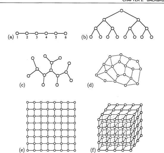
(e) 6-6-6-6-66-6-6 (f)

Figure 2.1. Drawings of several graphs. (a) chain, (b) hierarchical tree, (c) irregular tree, (d) planar

graph, (e) square lattice (also planar), (f) cubic lattice. In (a), we explicitly label the vertices V = {1, 2,3,4,5,6}. The edges of this graph are g = { {1,2}, {2,3}, {3,4}, {4,5}, {5,6} }.

variables. The conditional distribution of x given y is defined P(xly) = P(x, y)/P(y) for all y such that P(y) > 0.

We may define a matrix A to have matrix elements aij by writing A = (aij). Given a function f (0) = f (01,..., Od) of parameters 0, we define the gradient of f as Vf(0) = I a)". The Hessian of f is defined as the matrix of second derivatives: V2f(0) =

a

2f(o). Given a vector map A : Rd - Rd, we define the Jacobian as

OA(O)

= (.A1(o) A set X C Rd is convex if Ax + (1 - A)y E X for all x, yeX and 0 < A < 1. A function f : X -- R is convex if f(AX + (1 - A)) < Af (x) + (1 - A)f(y). It is strictly convex if f(Ax + (1 - A)) < Af(x) + (1 - A)f(y) for all x 0 y and 0 < A < 1.

(27)

Sec. 2.2. Introduction to Graphical Models

m m m 1

I I I

(a)

1

2 3 4 5 6

(b)i 0

L

L0

(c)

(d'

Figure 2.2. Drawings of several hypergraphs (using the factor graph representation). (a) a

3rd-order chain, (b) irregular 3rd-3rd-order edges and singleton edges, (c) irregular hypergraph, (d) hierarchical hypergraph having 3rd-order edges between levels, pairwise edges within each level and singleton edges at the bottom level. In (a), we explicitly label the vertices V = {1, 2, 3, 4, 5, 6}. The edges of this graph are 9 = { {1,2,3}, {2,3,4}, {3,4,5}, {4,5,6} }

N

2.2 Introduction to Graphical Models

* 2.2.1 Graphs and Hypergraphs

Although we do not require very much graph theory, the language of graphs is essential to the thesis. We give a brief, informal review of the necessary definitions here, mainly to establish conventions used throughout the thesis. Readers who are unfamiliar with these concepts may wish to consult the references [20,33,105]. A graph is defined by a set of vertices v E V (also called the nodes of the graph) and by a set of edges E E

g

defined as subsets (e.g., pairs) of vertices.1 Edges are often defined as unordered2

pairs of vertices {u,

v}

E G. Such pairwise graphs

g

C

(y)

are drawn using circle

nodes to denote vertices and lines drawn between these nodes to denote edges. Several such drawings of pairwise graphs are shown in Figure 3.3. We also allow more general definitions of graphs

g

C 2V \

0,

also known as hypergraphs [20], for which edges (also called hyperedges) may be defined as any subset of one or more vertices. To display such a generalized graph, it is often convenient to represent it using diagrams such as

1_{We deviate somewhat from standard notation}_g₌

(V, E) where

9

denotes the graph and E denotes the edge set of the graph. We instead use g to denote both the graph and its edge set, as the vertex set V should be apparent from context.

2

This definition is for undirected graphs. It is also common to define directed graphs, with edges defined as ordered pairs (u, v) E

g.

A directed edge (u, v) is drawn as an arrow pointing from node u to node v. We focus mainly on undirected graphs in this thesis.

(28)

seen in Figure 2.2. In these diagrams, each circle again represents a vertex v E V of the graph but we now use square markers to denote each edge E E G. The structure of

g

is encoded by drawing lines connecting each edge E E

g

to each of its vertices v E E. There is one such connection for each pair (v, E) E V x 9 such that v E E. Such representations are called factor graphs in the graphical modeling and coding literatures [85,153].

(Generalized) Graph Convention Unless otherwise stated, when we refer to a graph

g

or an edge E E

g,

then it should be understood that

g

may be a generalized graph (a hypergraph) and E may be any subset of one or more edges (a hyperedge). This includes the usual definition of pairwise graphs as a special case, and most of our examples and illustrations do use pairwise graphs to illustrate the basic ideas. Allowing

g

to possibly be a hypergraph in general allows us to express the general case without having to always use the more cumbersome terminology of "hyergraph" and "hyperedge" throughout the thesis. If it is essential that a given graph is actually a pairwise graph, then we explicitly say so. We occasionally remind the reader of this convention by referring to

g

as a

"(generalized) graph".

We now define some basic graphical concepts. Note, although these definition are often presented for pairwise graphs, the definitions given here also apply for generalized graphs (unless otherwise noted). A subgraph of

g

is defined by a subset of vertices Vsub C V and a subset of edges gsub C

g

such that each edge is included in the vertex set (we also say that

g

is a supergraph of gsub). Unless otherwise stated, the vertex set is defined by the union of the edges of the subgraph. The induced subgraph 9A based

on vertices A C V is defined as the set of all edges of g that contain only vertices in

A. A clique is a completely connected subset of nodes, that is, a set C C V such that

each pair of nodes u, v E C are connected by an edge, that is, u, v E E for some E E G. A path of length

e

is a sequence of nodes (vo, ... ,ve) and edges (E1,..., Ee) such that

no node or edge is repeated (except possibly vo = vy) and consecutive nodes (vk, Vk+l)

are contained in their corresponding edge Ek. This path connects nodes vo and vy. If vo = vi we say that the path is closed. A graph is connected if any two nodes may be connected by a path. The connected components of a graph are its maximal connected subgraphs. A cycle is a subgraph formed from the nodes and edges of a closed path. A tree is a connected, pairwise graph that does not contain any cycles (see Figures 3.3(a), (b) and (c)). A pairwise graph is planar if it can be drawn in the plane without any two edges intersecting (see Figures 3.3(d) and (e)).

Some additional definitions are presented as needed in later sections. Graph sep-arators are defined in Section 2.2.3. Chordal graphs and junction trees are discussed in Section 2.4.1. Also, several canonical graphical problems (max-cut, max-flow/min-cut, maximum-weight independent sets and maximum perfect matching), which arise in connection with MAP estimation, are briefly discussed in Section 2.5.

(29)

Sec. 2.2. Introduction to Graphical Models

* 2.2.2 Graphical Factorization and Gibbs Distribution

Let x = (Xi,...,, Xn) E Xn be a collection of variables where each variable ranges over the set X.3 For example, a binary variable model is given by X = {0, 1} and a continuous variable model has X = R. We define a graphical model [43, 60, 145] as a probability model defined by a (generalized) graph

g

with vertices V = {1,... , n}, identified with variables xl,..., xn, and probability distributions of the form

P(x) 1

1

E(XE)

(2.1)

Eeg

where each /E : XE -- R is a non-negative function of variables XE = (xv, v E E) and Z(4) is a normalization constant.4 We call the individual functions OE the factors of the model. In the factor graph representation (Figure 2.2), each circle node v E V represents a variable z, and each square node E E

g

represents one of the factors bE.

For strictly positive models (P(x) > 0 for all x) the probability distribution may be equivalently described as a Gibbs distribution of statistical physics [90,129,173,195], expressed as

P(x) =

exp

03

fE(XE)

(2.2)

Z(f,)

_E

where f(x) = EE fE(XE) is the energy function (or Hamiltonian) and the individual terms fE(XE) are called potential functions (or simply potentials) of the model.5 _The

parameter3 > 0 is the inverse temperature of the Gibbs distribution and

Z(f,

i3

)

E exp

fE(XE)

(2.3)

XEXn L EE9 )

is the partition function, which serves to normalize the probability distribution. Evi-dently, the probability distributions defined by (2.1) and (2.2) are equivalent if we take

PE(XE) = exp{fE(XE)} (and

3

= 1). In statistical physics, the free energy is defined as F(O,

/)

0/- 1 log Z(f,

/),

which (for

/

= 1) is also called the log-partition function in the graphical modeling literature. Later, in Section 2.3.2, we discuss the relation of this quantity to Gibbs free energy . The temperature 7 =

/

- 1 _{may be viewed as a}

parameter that, for a fixed energy function f(x), controls the level of randomness of

3

More generally, each variable may have a different range of values Xi such that x e X1 0X2 ... 0 X~. 4

We use the notational convention that whenever we define a function of variables x (x,, v V)

in terms of functions defined on subsets S C V of these variables, we use xs = (x, v E S) to denote a subset of the variables x (x and XA are not independent variables). Likewise, fA (XA) + fB (XB) should be regarded as a function of the variables XAUB. If S & A n B is non-empty, then the variables xS are shared by fA and fB.

5

For notational convenience, our definition of energy and potential functions are negated versions of what is normally used in physics (the definition of the Gibbs distribution normally includes a minus sign in the exponent).

Convex relaxation methods for graphical models : Lagrangian and maximum entropy approaches

Convex Relaxation Methods for Graphical Models:

Lagrangian and Maximum Entropy Approaches

by

ARCHIVES

IOCT 2 2 2WA

LIBRARIES

--Convex Relaxation Methods for Graphical Models:

Lagrangian and Maximum Entropy Approaches

Abstract

Acknowledgments

Contents

Chapter 1

Introduction

U 1.1 Motivation and Overview

* 1.2 Related

Work

* 1.2.1 MAP Estimation

* 1.2.2 Learning Graphical Models

4o

* 1.3 Contributions

E

1.3.1 Lagrangian Relaxation for MAP Estimation

* 1.3.2 Maximum Entropy Relaxation for Learning Graphical Models

U 1.4 Organization

Chapter 2

Background

* 2.1 Preamble

0

Ix

f(x).

(d)

I I I I I I I I

0--

I

l l l l l l

---0---0

I

a

OA(O)

I I I

(a)

1

(b)i 0

L

L0

(c)

(d'

2.2 Introduction to Graphical Models

* 2.2.1 Graphs and Hypergraphs

g

pairs of vertices {u,

E G. Such pairwise graphs

g

C

(y)

are drawn using circle

g

0,

9

g.

g

g

g

g,

g

g

g

g

g

g

e

* 2.2.2 Graphical Factorization and Gibbs Distribution

g

1

(2.1)

g

P(x) =

exp

03

_I

_{l l l l l l}

_I

_E