A cut-cell method for adaptive high-order discretizations of conjugate heat transfer problems

(1)

A Cut-Cell Method for Adaptive High-Order Discretizations

of Conjugate Heat Transfer Problems

by

Steven Matthew Ojeda

B.S.,

Massachusetts Institute of Technology (2012)

Submitted to the Department of Aeronautics and Astronautics

in partial fulfillment of the requirements for the degree of

OF TECHNOLOGY

Master of Science in Aeronautics and Astronautics

JUN 16 2014

at the

IBRARIES

MASSACHUSETTS INSTITUTE OF TECHNOLOGY

June 2014

©

Massachusetts Institute of Technology 2014. All rights reserved.

Author ...

Signature

...

Department of Aeronautics and Astronautics

May 22, 2014

ISignature

redacted

C ertified by

...

David Darmofal

Professor oYAeronautics and Astronautics

Thesis Supervisor

Signature

redacted-A ccepted by ....

...

Paulo C. Lozano

Associate Professor of Aeronautics and Astronautics

Chair, Graduate Program Committee

(2)

(3)

A Cut-Cell Method for Adaptive High-Order Discretizations

of Conjugate Heat Transfer Problems

by

Steven Matthew Ojeda

Submitted to the Department of Aeronautics and Astronautics on May 22, 2014, in partial fulfillment of the

requirements for the degree of

Master of Science in Aeronautics and Astronautics

Abstract

Heat transfer between a conductive solid and an adjacent convective fluid is prevalent in many aerospace systems. The ability to achieve accurate predictions of the coupled heat interaction is critical in advancing thermodynamic designs. Despite their growing use, coupled fluid-solid analyses known as conjugate heat transfer (CHT) are hindered

by the lack of automation and robustness. The mesh generation process is still highly

dependent on user experience and resources, requiring time-consuming involvement in the analysis cycle. This thesis presents work toward developing a robust PDE solution framework for CHT simulations that autonomously provides reliable output predictions. More specifically, the framework is comprised of the following compo-nents: a simplex cut-cell technique that generates multi-regioned meshes decoupled from the design geometry, a high-order discontinuous Galerkin (DG) discretization, and an anisotropic output-based adaptation method that autonomously adapts the mesh to minimize the error in an output of interest.

An existing cut-cell technique is first extended to generate fully-embedded meshes with multiple sub-domains. Then, a coupled framework that combines separate dis-ciplines is developed, while ensuring compatibility between the cut-cell and mesh adaptation algorithms. Next, the framework is applied to high-order discretizations of the heat, Navier-Stokes, and Reynolds-Averaged Navier-Stokes (RANS) equations to analyze the heat flux interaction. Through a series of numerical studies, high-order ac-curate outputs solved on autonomously controlled cut-cell meshes are demonstrated. Finally, the conjugate solutions are analyzed to gain physical insight to the coupled interaction.

Thesis Supervisor: David Darmofal

(4)

(5)

Acknowledgments

I would like to express my sincere gratitude to all people who have made this thesis

possible. First, I would like to thank my advisor, Prof. David Darmofal, for providing me with the opportunity to learn from and contribute to the CFD community, and for encouraging me during my graduate study. In addition, I would like to thank Dr. Steven Allmaras for his very knowledgeable insight and continued commitment to my weekly meetings. I would also like to recognize Marshall for teaching me the tools of the trade, and for providing me with the continuous feedback I needed to learn.

This thesis would not have been possible without the relentless efforts of the entire ProjectX team. I would like to thank past members who had built the building blocks and who had contributed many years of their lives developing ProjectX. I would also like to thank: Huafei for helping me climb the learning curve, and for laying down the foundation of my work; Jun and Phil for their unbounded willingness to help solve problems, share ideas, and drink coffee with me; Carlee, Savi, Yixuan, and Jeff for bringing new perspectives to the team. Thank you all, and the best of luck to you.

I would like recognize people in the ACDL for creating a productive working

environ-ment: David M, Xevi, Ferran, and Hemant for sharing their ideas and encouragement; Patrick for making me take breaks for coffee hour; Eric for his admin support and sense of humor. I would like to thank all my friends outside the ACDL: the brothers of Theta Chi for always extending a helping hand; Giulia and Ed (team WindX) for encouraging me with their positivity and puns; Andras for his problem solving and cooking skills; among many more. I would also like to give a special thanks to Erica for inspiring me to summit my goals, strive for a healthy lifestyle, and reframe all frustrating scenarios into positive ones.

Lastly, I would like to thank my family - Mom, Dad, and Laura - for their

uncondi-tional love and support. The past few years have been quite difficult, and I would not be where I am today without their continuous guidance and encouragement. I wish

(6)

you many years of joy and health, and I am excited to be moving closer to home. Finally, I would like to acknowledge the financial support provided by the Boeing Company (technical monitor Dr. Mori Mani), the MIT Graduate Work Program, and the MIT AeroAstro Department through fellowships.

(7)

List of Figures

1-1 Example of a cut-cell mesh . . . .

1-2 Automated process of the output-based adaptive PDE solver

2-1 Multi-region interface example . . . .

2-2 Multi-region geometry representation . . . .

2-3 Background and cut mesh . . . .

2-4 Example of zerod and oned objects in a multi-region intersection .

2-5 Formation of twod types in a multi-regioned cut element . . . . .

3-1 3-2 3-3 3-4 3-5 3-6 3-7

Example of mesh to continuous metric field mapping . . . .

Example split configurations with respective metric tensors (Yano

[77])

Example split configurations for cut elements (Sun

[71])

. . . .

Example of vertex layer (grey represents null region) . . . .

Background mesh for r' singularity problem . . . . Optimized meshes for r' singularity problem with 4000 DOF . . . . .

Metric distribution for r' singularity problem with a = 2/3 . . . .

4-1 Sketch of NS solid wall interface states used to compute numerical fluxes 4-2 Compressible Poiseuille flow model . . . . 4-3 Numerical solution to the compressible Poiseuille flow with variable P

an d r . . . . .

4-4 Temperature and corresponding viscosity variation for compressible Poiseuille flow . . . .

4-5 Uniformly refined meshes . . . .

20 24 30 31 32 36 37 48 50 52 53 54 55 56 59 61 64 65 66

(12)

4-6 4-7 4-8 4-9 4-10 4-11 4-12 4-13 4-14 4-15 4-16 4-17 4-18 4-18 4-19 4-20 4-21 4-22 4-23 4-24 4-25 4-26 4-27 4-28 4-29 4-30 4-31 4-32 4-33 4-34

Convergence of the density L2 error. . . . . 67

Poiseuille flow drag adaptation history for 16k DOF . . . . 69

Poiseuille flow drag adapted meshes . . . . 70

Poiseuille flow drag adapted error convergence . . . . 71

Poiseuille flow heat flux adaptation history for 16k DOF . . . . 72

Poiseuille flow heat flux adapted meshes . . . . 72

Poiseuille flow heat flux adapted error convergence . . . . 73

Poiseuille flow comparison of drag vs. heat flux adaptation . . . . 74

Cooled nozzle flow model . . . . 75

Numerical solution to the cooled nozzle flow . . . . 77

Temperature solution to the cooled nozzle flow . . . . 77

Cooled nozzle drag adaptation history for 16k DOF . . . . 78

Cooled nozzle drag adapted meshes . . . . 79

Cooled nozzle drag adapted meshes zoom . . . . 80

Cooled nozzle drag adapted error convergence . . . . 80

Cooled nozzle heat flux adaptation history for 16k DOF . . . . 81

Cooled nozzle heat flux adapted meshes . . . . 82

Cooled nozzle heat flux adapted meshes zoom . . . . 82

Cooled nozzle heat flux adapted error convergence . . . . 83

Cooled nozzle comparison of drag vs. heat flux adaptation . . . . 84

Multi-regioned flow model . . . . 85

Numerical solution to the multi-flow problem . . . . 87

Temperature solution to the multi-flow problem . . . . 87

Multi-flow 24k DOF heat flux adaptation history . . . . 88

Multi-flow heat flux adapted meshes . . . . 89

Multi-flow heat flux adapted meshes zoom . . . . 90

Multi-flow heat flux adapted error convergence . . . . 91

Multi-flow 24k DOF normalized mass flux adaptation history . . . . . 92

Multi-flow mass flux adapted meshes . . . . 92

(13)

4-35 4-36

Multi-flow mass flux adapted error convergence . . . . 93

Multi-flow adapted mesh comparison (NOT TO SCALE) . . . . 94

5-1 Sketch of RANS solid wall interface states used to compute numerical fluxes... ... 5-2 RANS Slab flow model . . . . 5-3 Numerical solution to RANS Flat Slab p=2 26k DOF . . . . 5-4 Vertical slices of normalized solutions to RANS Flat Slab p=2 26k DO 97 99 100 F101 5-5 Interface thermal profile for RANS Flat Slab p=2 26k . 5-6 RANS Flat Slab heat flux adaptation history . . . . 5-7 RANS Flat Slab heat flux adapted mesh . . . . 5-8 RANS Flat Slab heat flux adapted mesh correlation . . 5-9 Backward-facing step conjugate flow model . . . . 5-10 Numerical solution to BFS p=2 50k DOF . . . . 5-11 Interface profiles for BFS p=2 50k DOF . . . . 5-12 BFS heat flux adaptation history over range of O's . . . 5-13 BFS heat flux adapted meshes . . . . 5-14 BFS heat flux adapted meshes zoom . . . . 5-15 Numerical solution to BFS p=2 50k DOF zoom . . . . 5-16 Moffatt Vortices p=2 50k DOF . . . . 5-17 Mesh refinement of 'updraft' in BFS recirculation bubble . . . . 102 . . . . 103 . . . . 104 . . . . 105 . . . . 107 . . . . 109 . . . . 111 .. .... 112 . . . . 113 . . . . 114 . . . . 115 . . . . 116 (p=2 50k DOF)117 B-1 Transformed Coordinates . . . . 133

C-1 RANS flat slab heat flux adapted mesh . . . . 139

C-2 RANS flat slab adjoint profiles . . . . 140

C-3 RANS flat slab normalized boundary layer profiles . . . . 141

(14)

(15)

List of Tables

2.1 2D multi-region geometry attributes . . . . 30

2.2 Information stored for zerod objects . . . . 34

2.3 Information stored for oned objects . . . . 34

(16)

(17)

Chapter 1 Introduction

1.1 Motivation

Numerical simulation has become a critical tool for engineering analysis over the last several decades. In particular, Computational Fluid Dynamics (CFD) software has widely been used throughout academia and industry to analyze and drive aerospace design. As an alternative to experimental testing for certification, CFD offers rela-tively fast turnaround times and the ability to simulate a wide range of component designs and test conditions. Additionally, with recent advancements in algorithm de-velopment and increased computational power, CFD solvers are becoming far more capable in analyzing problems with complex geometry, physics, or both. However, de-spite their widespread use, many CFD software packages still lack efficiency, reliability, and autonomy, yielding unaffordable high-fidelity simulations, unreliable predictions in outputs of interest, and heavy user involvement.

Depending on the size of the problem and the computational resources being used, common high-fidelity simulations can take hours or even days to complete. Equally inhibiting, user involvement is dominated by two factors: (1) the process of under-standing and determining where mesh refinement is necessary in order to achieve an accurate solution, and (2) the process of generating a corresponding mesh to conform with the modeled geometry, which can take weeks to even months depending on the

(18)

geometry complexity. Worse still, unreliable predictions in outputs of interest com-pounded with the absence of solution uncertainty quantification greatly impairs the validity of the solution, diminishes the value of the expensive analysis cycle, and can even lead to large-scale disasters. For example, the 44,000-ton Sleipner A offshore platform sank in 1991 due to a flawed design. Costing $700 million, this failure was caused by a finite element analysis that underestimated the shear stress in a concrete

support structure by 45 % [38]. After further investigations, it was found that the

underestimation resulted from an under-resolved mesh with poorly shaped elements. The analysis was performed again with a suitable mesh, and returned with a pre-dicted structural failure occurring at a water depth of 62 meters, agreeing closely with the actual failure depth of 65 meters [24]. Hence, the lack of reliability in the mesh generation and error estimation process led to a catastrophic failure that could have been avoided with proper error control.

Fortunately, mesh adaptation offers a means toward mitigating mesh reliance on hu-man experience, and instead provides a far more reliable output prediction through a systematic and autonomous control over the error. In conjunction, higher-order dis-cretizations, which are becoming more prevalent in the CFD community, can further improve the solution and output accuracy. Despite these promises, however, the mesh generation process in an industry setting still serves as a primary 'bottleneck' in the CAD-to-mesh-to-solution cycle [26]. A couple difficulties contributing to this bottle-neck involve: requiring curved elements to conform to the geometry surface in order to

maintain the benefit of higher-order discretizations [7], and achieving different levels

of refinement in specific areas within the domain.

In the context of multi-disciplinary simulations where multiple governing partial dif-ferential equations (PDE's) are solved simultaneously, many of the mesh generation and error control issues are exacerbated by the complexity of the coupled problem. The ability to sufficiently resolve important regions in the domain is non-trivial for single disciplines, let alone multiple disciplines. Often times, many industry simu-lations that involve solid bodies interacting with fluid flow simplify the problem by

(19)

assuming conditions that decouple the two domains, such as using adiabatic walls or a constant heat flux assumption, as oppose to solving the fully coupled conjugate heat transfer (CHT) problem. Certainly, if the thermal variation within the solid is negligible, these assumptions may apply; however, many aerospace applications consist of thermal-fluid interactions that are highly coupled, and reliable solutions cannot be obtained if the assumptions are maintained. Instead, a robust and au-tonomous method for generating multi-disciplinary, adapted meshes is necessary to conduct efficient CHT simulation. With the help of mesh adaptation, the ability to accurately capture the coupled interaction between a fluid and solid can foster and facilitate aerospace design by:

" mitigating crack development due to thermal shocks

" reducing hot spots in high-temperature environments " allowing reductions in coolant flows

" determining performance metrics for heat exchangers " increasing accuracy in predicted heat transfer coefficients " optimizing highly coupled thermal-fluid component design

With these applications in mind, this thesis presents work toward: streamlining the CAD-to-mesh-to-solution cycle through a cut-cell technique, utilizing high order dis-cretizations, and integrating an error estimation and adaptation process for multi-disciplinary conjugate heat transfer problems.

1.2 Background

1.2.1 Cut-Cell Methods

The mesh generation process for unstructured grids is often very time-consuming, and also suffers from robustness issues involving highly anisotropic elements around high-order curved geometries. One alternative for a streamlined and robust process is the use of cut cells, where the computational mesh is 'cut' from a background

(20)

mesh that is not required to conform to the geometry at hand. This process begins with the generation of a coarse background mesh, which is then intersected with a non-conforming geometry, or embedded geometry, to create a cut-cell mesh consisting of arbitrarily shaped elements. Depending on the type of problem, the embedded geometry may specify a solid body embedded in an external flow (in which case the external mesh becomes the computational domain), or it may specify the outer boundaries of a fully embedded domain (in which case the interior mesh becomes

the computational domain). FIGURE 1-1 illustrates an example of the latter, where a

fully embedded cut-cell mesh is formed from a background mesh intersecting with an arbitrary embedded geometry. Without the requirement of boundary conformity, the generation of a cut-cell mesh now only relies on an automated intersection algorithm. However, the burden of robustness is transferred to the PDE solver, which must now account for the resulting arbitrarily shaped elements within the cut-cell mesh. Despite this added complexity, the automated benefits of the cut-cell technique may still outweigh the large cost associated with a traditional boundary-conforming mesh generation process.

(a) Background mesh (b) Arbitrary geometry

(c) Cut mesh from embedded geometry

(21)

The initial concept of cut-cell methods was first considered by Purvis and Burkhalter

[62] in 1979. In their work, the full potential equations were solved on cut

Carte-sian background meshes, which has more recently been extended to 3D meshes with complex boundaries. For example, Young et al. [80] demonstrated an accurate and reliable method for solving the 3D potential flow equations on complex geometry. Their Cartesian cut-cell finite element method used Stokes' theorem to carry out the volume integration of linear cut cells, and allowed for adaptation based on geometric

or solution features. Furthermore, Karman [43] had developed software (SPLITFLOW)

that used a Cartesian grid to solve the 3D Reynolds-Averaged Navier-Stokes (RANS) equations. However, this technique required a priori knowledge of the location and orientation of dominant flow features in order to properly align the Cartesian grid. As such, Cartesian grids are limited in the direction in which anisotropic elements are desired, and are therefore inefficient in resolving anisotropic features in Navier-Stokes and RANS problems.

To overcome this limitation, Fidkowski and Darmofal developed a simplex cut-cell method for 2D and 3D embedded boundary problems [32]. Combined with a high-order discontinuous Galerkin discretization, this method used cubic splines to repre-sent embedded geometries in two dimensions, and quadratic patches in three dimen-sions. The method enabled anisotropic adaptation, though exhibited low quadrature quality in arbitrarily shaped cut cells, and ill-conditioning due to small volume ratios between element neighbors. Since then, robustness and automation improvements of the method have occurred. For instance, Modisette developed an algorithm to recognize canonical shapes for cut cells in two dimensions to improve their respective quadrature quality, as well as a merging technique to improve the overall condition-ing [51]. Additionally, Sun introduced the use of magic points for cut-cell quadrature rules, and demonstrated the method on interface problems [72].

This improved cut-cell method becomes particularly useful in 'multi-regioned' simula-tions, where generating interface-conforming meshes becomes far more challenging as the number of region boundaries and interfaces increase. Several methods, such as the

(22)

immersed interface method [46] and ghost fluid method [30], have been developed to handle non-interface-conforming meshes, though are typically second-order accurate. In order to achieve high-accuracy solutions to interface problems, the method must be compatible with high-order discretizations [71]. Though the cut-cell method by Sun produces meshes to obtain high-order solutions to a single interface problem, the algorithm is not capable of generating cut-cell meshes for multi-disciplinary domains with an arbitrary number of boundaries and interfaces. Hence, Sun's cut-cell method is used as a starting point for developing a method to streamline the mesh generation process for multi-regioned, high-order conjugate heat transfer problems.

1.2.2 High-Order Discretizations

The primary goal of high-order methods is to achieve higher fidelity solutions at a fraction of the cost of low-order methods. Because of their ability to reduce discretiza-tion error, high-order methods become important in complex problems that require high accurate solutions. As an example, a heat transfer review by Peniguel illumi-nates common low-order methods that overestimates the average Nusselt number of a heated flat plate case by a factor of two [58]. Not only that, Peniguel expresses that this overestimation is typical for industry RANS solvers. With the added complex-ity of a strongly coupled conjugate heat transfer problem, the abilcomplex-ity to control the discretization error is paramount.

Most aerospace industry CFD methods today can only achieve second order error

convergence defined as E oc 0(h2), where E is a measure of the error, and h is a

measure of the mesh size. Generally speaking, high-order refers to a discretization's ability to obtain a higher convergence rate r in order to achieve improved accuracy. More specifically, high-order methods typically achieve error convergence rates that

are higher than second order: E oc 0(hr>2_),_{for an L}2_{-error measure.}

In this work, finite element schemes are used to achieve high-order discretizations as they are applicable to unstructured meshes, which can more readily tessellate models

(23)

with complex boundary or interface geometry. They also offer an elegant extension to high-order accurate solutions by increasing the order of basis polynomials. The concept of increasing the polynomial order p (while maintaining a constant grid spac-ing, h) is known as a 'p-type' method, which had originally been applied to elasticity equations in 1981 by Babuska et al. [4]. Their study found that the p-type method required fewer degrees of freedom to achieve a similar level of accuracy when applied to smooth problems. In order to realize the benefits of high-order methods for prob-lems with low regularity, however, h-type methods (one that adapts the grid spacing) are required to control the resulting discretization error. For instance, Yano et al.

[79] demonstrated the affordability of high-order convergence by solving compressible

Navier-Stokes and RANS problems with a mesh adaptation method.

To stabilize the finite element discretization for convection-dominated problems, the discontinuous Galerkin (DG) method is used. The DG method dates back to 1973, where Reed and Hill first introduced it for scalar hyperbolic equations [63]. Soon af-ter, LeSaint and Raviart [45] proved that, assuming a smooth solution with a p-order

polynomial basis, the L2_{-error of the DG method is O(hP), while Richter [64] proved}

a decade later that convergence rates of O(hP+l) can be obtained. The method was later extended to nonlinear hyperbolic problems by Chavent and Salzano [18] using Godunov's flux, followed by an extension to using a Runge-Kutta explicit time in-tegration (RKDG) by Cockburn, Shu, and co-authors [21, 20, 19, 22]. For solving elliptic problems, Arnold and Wheeler [3, 76] developed interior penalty methods, while Bassi and Rebay later developed the so-called BRI [8] and BR2 [9] discretiza-tions. The BR2 scheme achieves stability for purely elliptic problems, and serves as the viscous discretization, in this work.

1.2.3 Output-Based Error Estimation and Mesh Adaptation

Many engineering applications require the development of high-fidelity models to accurately predict an output of interest. This development typically involves the generation of a mesh that, through experience, is refined in areas that reduces the

(24)

output error. For complex problems (including CHT), experience is not enough to locate regions needing refinement a priori. Hence, an output-based adaptation frame-work that resolves appropriate domain features in the absence of human experience is desired. Combined with a high-order discretization and a cut-cell method framework, mesh adaptation could enable a user to specify a required error level and a maximum

allotted time for an automated multi-disciplinary simulation. FIGURE 1-2 illustrates

an ideal flow of information to achieve an output of interest within a desired error tolerance, Ema, and a desired solve time, rma. For a multi-disciplinary problem, the process begins with a cut-mesh generated by intersecting the multi-regioned geometry with an initial (coarse) background mesh. Next, the discretized PDE's are solved on the new cut-mesh, followed by an estimation of the resulting output error. If the error or time tolerances are not met, the estimated error is localized on an elemental level, and the background mesh is adapted to reduce the error. This process continues until the outputs reach an acceptable error level, or the run-time is exhausted. The three primary modules in this process are the cut-cell framework (as discussed earlier), the output error estimation, and the mesh adaptation procedure.

FIGURE 1-2: Automated process of the output-based adaptive PDE solver

Error Estimation

The purpose of error estimation in the adaptive process is to first determine a global error to assess the validity of an output of interest, then localize the error to identify which elements contribute to the global error the most. Several varieties of error estimation have been developed to achieve these goals. A common strategy is to

(25)

identify dominant solution features based on the areas marked by large gradients,

as shown by Baker [5]. However, large gradients in a solution do not necessarily

localize the area of greatest error. For example, small upstream perturbations can have an effect on downstream features, despite the largest gradients occurring in the

downstream features

[75].

Another method is residual-based error estimation, which

relies on calculating residual norms that bound the error. Though this method was demonstrated to function well in one-dimensional transonic flows with shocks [81], it has not been proven successful in two dimensions.

An improved method consists of an output-based error estimation technique that localizes the output error by incorporating the corresponding adjoint solution from the dual problem. The adjoint serves as the sensitivity of an output of interest to perturbations in the primal residual, which links the output error to the local residual. Such method is given by the dual-weighted residual (DWR) method proposed by Becker and Rannacher [11, 12], and is used in this work to drive mesh adaptation. The DWR method has been extended and implemented for several mesh adaptation procedures, notably the first output-based, anisotropic adaptation method applied to

RANS problems by Venditti and Darmofal [73].

Mesh Adaptation

Given a localized error estimate, the purpose of mesh adaptation is to minimize the

output error by changing the mesh spacing (h-type adaptation). In other words, given an amount of resources (degress of freedom), the best approximation of the output of interest can be determined by controlling the error through mesh optimization. For purely isotropic adaptation, the localized error from the DWR method is sufficient to carry out a fixed fraction strategy. This technique first ranks all elements within the computational domain by their localized error, then performs a refinement of those with the highest error, and a coarsening of those with the lowest error. However, to generate efficient meshes for high-Reynolds flows where boundary layers, wakes, and shocks require a resolution with high aspect ratios, anisotropic meshes are needed.

(26)

One way to represent an anisotropic mesh is to formulate the mesh information as a metric tensor field that defines the size, stretching, and orientation of each element. Though an anisotropic mesh can be fully characterized by a conforming metric field, it still belongs to a family of metric-conforming meshes that all have similar approx-imation properties [48, 49]. Given a metric field, several anisotropic mesh generators such as BAMG [14, 37] can be used to generate corresponding meshes. This way, an anisotropic mesh that conforms to a desired distribution that reduces the total output error is possible. Peraire et al. [60] developed a method based on the Hessian of a solution field to control the anisotropic mesh configuration. Venditti and Dar-mofal [73] proposed an anisotropic adaptation method that relies on both the DWR method and an anisotropy detection based on the Hessian of the Mach number, while Fidkowski and Darmofal [32] extended this idea to high-order discretizations.

Beyond this, Yano and Darmofal [78] proposed the Mesh Optimization via Error Sampling and Synthesis (MOESS) algorithm, which determines adapted meshes by solving a continuous constrained optimization problem. This is done by formulating the objective as the output error, and defining the design variables as the degrees of freedom in a metric tensor field. The error-metric sensitivities are approximated by first constructing split configurations for each element, then solving for the resulting error for each configuration. As defined, this method is only capable of performing error sampling over triangular elements, and therefore cannot be used for arbitrarily shaped elements. However, Sun has extended this method to handle cut-cell meshes for embedded boundary problems [71], and performs the adaptation procedure on the background mesh. Additionally, Kudo [39] has modified the mesh adaptation method to use a gradient-based optimization algorithm.

In the context of multi-disciplinary problems, mesh adaptation is important in re-solving anisotropic and perhaps non-intuitive features in each sub-domain. Since multi-regioned domains are tessellated using a cut-cell mesh, and the mesh adapta-tion process is performed on the background mesh, the modificaadapta-tion and generaadapta-tion of a new optimized mesh is completely decoupled from the geometry at hand. Hence,

(27)

the combined cut-cell and mesh adaptation framework allows for efficient and au-tonomous output error minimization of multi-regioned domains, and is demonstrated in this thesis for conjugate heat transfer problems.

1.3 Thesis Overview

This thesis presents work toward developing a robust, PDE solution framework for

CHT simulations that autonomously provides reliable output predictions. In

partic-ular, the framework is comprised of three primary components: a simplex cut-cell technique, a high-order DG discretization, and an anisotropic output-based adapta-tion method. The specific contribuadapta-tions of this thesis are as follows:

* Extension of cut-cell methods to fully-embedded, multi-regioned domains.

" Development of a coupled framework that combines separate disciplines,

com-patible with the integrated cut-cell and mesh adaptation methods.

" Demonstration of the CHT framework with high-order discretizations of the

heat, Navier-Stokes, and RANS equations.

In this thesis, CHAPTER 2 details the cut-cell algorithm used to generate

multi-regioned meshes. CHAPTER 3 provides background for the DG discretization,

dual-weighted residual output error estimation, and mesh optimization with cut-cell

ex-tensions. In CHAPTER 4, the CHT framework for the coupled heat and Navier-Stokes

equations is demonstrated, while CHAPTER 5 demonstrates the CHT framework for

(28)

(29)

Chapter 2 Multi-Disciplinary Cut Cell

Methods

Many aerospace applications rely on different analysis models to support and drive multi-disciplinary design. When coupled together, these analyses typically require computational meshes that are capable of representing different regions separated

by arbitrary interfaces. However, generating meshes that conform to the domain

boundary and interfaces can be very time-consuming if the geometry representation is complex. Cut-cell methods, on the other hand, do not require a mesh to conform to the interface geometry, and instead offer an alternative mesh generation process for multi-regioned domains. In this chapter, a two-dimensional cut-cell method for multi-regioned domains is presented.

2.1 Geometry Definition

For multi-disciplinary problems, the geometry consists of multiple boundaries and

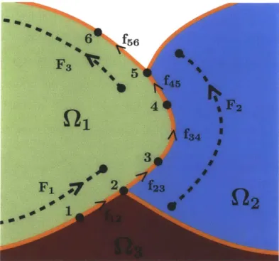
interfaces that form separate closed loop regions. FIGURE 2-1 illustrates an example

of a multi-regioned domain consisting of three regions, Q1, Q2, and Q3, separated by

interfaces, E13, E12, and E23. In two dimensions, these geometric features are uniquely

(30)

FIGURE 2-1: Multi-region interface example

Attribute Symbol Definition

Nodes ni (Xi, yi)

Faces fij (node i, node j)

Face Groups F {fjk}, (14, ri)

TABLE 2.1: 2D multi-region geometry attributes

The nodes are defined by a set of coordinates (Xi, yi), and the faces are defined by an

ordered nodal pair. The face groups are defined by both a set of faces, {fjk}, and a left

and right region index, 1i and ri, which corresponds to a user-specified material. Each face group F represents either an interface or boundary of the computational domain. As such, the user-supplied interface and boundary conditions for all interfaces and

boundaries in the domain are applied through the defined face groups. Each face fjk

in face group F must be oriented in the same direction such that the left and right

region on each face when traversing from node j to node k is equal to F's respective

left 1i and right ri region index. Additionally, all face groups are required to form a 'water-tight' geometry by establishing closed loops around each region. FIGURE 2-2 shows an example of the geometry representation for a multi-region interface domain.

Here, F2 consists of the set of faces: f23, f34, and f45, and region information: 12 = 1,

r2 = 2, that uniquely defines the interface between domain Q1 and Q2. Alternatively,

(31)

a null region, the corresponding region index is set to zero. For example, F3 in FIGURE 2-2 has an associated left and right region index: 13 = 1 and r₃ = 0, since

the left domain is Q, and the right domain is null. Note that face group directions can be defined in either direction, as long as its set of faces are oriented in the same direction, and its region information is consistent with the left and right domains.

FIGURE 2-2: Multi-region geometry representation

To approximate curvature in the geometry, cubic splines are used to represent all boundaries and interfaces defined by the face groups. At geometric corners or interface junctions where multiple regions intersect at a node, multiple splines are required to represent the geometry. Once all face groups are represented by splines, the geometry is used to generate a cut-cell mesh.

2.2 Cut-Cell Technique

The grid generation process for a cut-cell mesh begins with a background mesh,

(32)

the background mesh and embedded geometry definitions are not required to con-form, and are instead used to efficiently construct cut-cell meshes consisting of mul-tiple complex regions. Though conformity is not required, the geometry definition is

required to be fully embedded within the background mesh. FIGURE 2-3(a) shows an

example of an embedded domain within a non-conforming background mesh Th,b. To

create the cut-cell mesh, the geometry definition is intersected with Th,b, and Th,b is

separated or 'cut' into individual parts (T)) that reside completely within a single

region Qi. For instance, FIGURE 2-3(b) illustrates three elements of different regions,

C1, AC2, and C3, resulting from the intersection of the geometry with a single

back-ground element. Once a cut-cell mesh is created using the intersection algorithm, each element is either associated with a uniquely defined material or considered a null element (if outside the computational domain) in which case it is disregarded.

(a) Non-geometry-conforming background mesh (b) Example of elements cut from a

back-(grey signifies null region) ground mesh

FIGURE 2-3: Background and cut mesh

2.3 Multi-Region Intersection Algorithm

The generation of multi-region cut-cell meshes presented here is an extension of the intersection algorithm developed by Modisette [51], which creates cut elements on only one side of an interface to define a domain boundary. The algorithm also leverages the implementation provided by Sun [71] where cut elements are formed on both sides of an interface, creating two distinct domains. However, when generating cut meshes for n-regioned domains, junction points, which join multiple regions (ie. point

(33)

A

in FIGURE 2-3(b)), are encountered, warranting additional region information to precisely define the topology of the cut mesh. Hence, the algorithm utilizes region

information (li, r) that is specified for each face group F in order to identify and

create cut elements of unique regions.

To generate the cut mesh topology, the intersection algorithm starts by finding all

intersection points between the set of splines, indexed Sj = 1, 2, ..., nspline, and

back-ground mesh edges (ie. points B, C, and D in FIGURE 2-3(b)). For each spline, Si, a

bounding box method is used to detect all background mesh edges that are candidates for an intersection. In particular, the global coordinates of both the spline endpoints and any non-endpoint extrema (determined by solving a quadratic equation) are determined, and the maximum distance between the set of coordinates defines the di-agonal endpoints of the bounding box. The box is expanded slightly with a tolerance of max(O.Old, 10OMP) where d is the box diagonal length and MP represents machine precision, to ensure no intersections are missed. Then, the set of edges within the bounding box are determined by testing whether the edge endpoints are both within the box or, if not, whether the edges intersect the lines of the bounding box. For each edge within the bounding box, the intersection points are determined by solving a cubic-root problem with double precision arithmetic. Though it is possible to erro-neously detect an intersection due to floating point errors, the intersection between a spline and an edge is performed only once in order to prevent an inconsistent topology based on the ordering of the intersection calculations.

Junction points are determined by finding the nodes that share multiple face groups. Since multiple spline segments meet at junction points, the spline index, Sj, and spline

end parameter, send, of each joined spline are stored on the corresponding junction

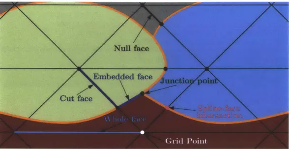
point. Both intersection and junction points, along with all other background grid points (ie. points S,Y, and g), are stored and referred to as zerod objects. Background faces that are "cut" by the intersection points are then formed into separate faces

called "cut" faces (ie. face 9N, B, etc. in FIGURE 2-3(b)). Additionally, spline

(34)

called "embedded" faces (ie. face BA A and A ). These faces, along with all other uncut background faces, or "whole" faces, are stored and referred to as oned

objects. TABLE 2.2 and TABLE 2.3 outline the different zerod and oned object types

along with their stored information, while FIGURE 2-4 shows an illustration of both

object types on a cut mesh.

zerod object Stored Information

Grid Point - Background grid node

- Single region index m

Junction Point - {Sj}, set of spline indices of joined spline segments

- {send}, set of spline parameters of joined spline ends

Spline-face intersection - Face index of background face

- Si, spline index of background spline segment - sin, spline parameter of intersection

TABLE 2.2 : Information stored for zerod objects

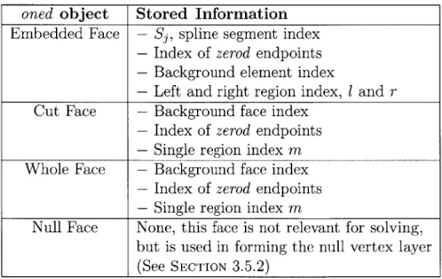
oned object Stored Information

Embedded Face - S, spline segment index

- Index of zerod endpoints

- Background element index

- Left and right region index, 1 and r

Cut Face - Background face index

Whole Face - Background face index

Null Face _{None, this face is not relevant for solving,}

but is used in forming the null vertex layer

(See SECTION 3.5.2)

TABLE 2.3: Information stored for oned objects

Oned objects are combined into elements by forming closed loops around single

re-gions. Each loop that is formed is referred to as a twod object, which defines a new cut element and its associated region. To create all loops within an intersected back-ground element, each "embedded" face must be traversed twice in opposite directions. The multi-regioned loop generation algorithm is detailed in ALGORITHM 1.

(35)

Algorithm: Multi-Regioned Loop Generation for

for all faces ej c OneD that is either an embedded face used less than twice or an unused cut face do

if (OneD[ej].zo Zcur) then

- Set ecur

- Set Zcur to OneD[ej].zi; else

if (OneD[ej].zi == Zcur) then

- Set ecur = ei;

- Set Zcur to OneD[ej1.zo; end

end end end end

- Assign region reur to the cut faces in the loop and to the newly constructed twod;

end end

Algorithm 1: Multi-region loop generation algorithm

each background element with an embedded geometry intersection Tc t do

- Set the used counter of all embedded faces to zero: ej.used = 0;

while not all embedded faces in T are used twice do

- Select an embedded face eo from a list of valid oned objects, OneD, associated with the

background element that has not been used twice;

if eo.used = 0 then (eo unused)

- Start a loop by traversing from the initial zerod on the embedded face, setting

Zstart = OneD[eo].zo, and Zcur = OneD[eo].zi;

- Set current region reur = OneD[eo].l;

else

(eo used once)

- Start a loop by traversing opposite to the direction previously used, setting Zstart OneD[eo].zi, and Zcur = OneD[eo].zo;

- Set current region rcur = OneD[eo].r; end

- Set ceur = eo and Zcur = OneD[eo].zi;

while (Zcur! = Zstart) do

- Add ecur to the Loop and increment used counter: ecur.used++;

if Zcur is a junction zerod then

for all embedded faces e C OneD used less than twice do

if (OneD[e<.zo Zcur) && (OneD[e ].l == rcur) then

- Set ecur

- Set zcur to OneD[e<.zi;

else

if (OneD[e<.zi == Zcur) && (OneD[e<.r rcur) then

- Set ecur = e ;

- Set zcur to OneD[e ].zo; end

end end else

(36)

FIGURE 2-4: Example of zerod and oned objects in a multi-region intersection

Since the algorithm can start with any embedded face eo, the order of the loop generation is not unique, though the algorithm guarantees a precise definition of the element topology when completed. As an example, FIGURE 2-5 shows the progression of the loop generation algorithm as the twod objects in a multi-regioned background element are constructed. To create twodi, the algorithm starts with an embedded

face, BA, and steps to junction point A. At the junction point, all oned objects

within the element are looped over, and the embedded face corresponding to the

current region, which in this case is A with 1 = 1, is selected. This is continued

until the closed loop is formed. Next, the cut faces, and g, and the twod object,

BACg, is assigned with the region index m = re,, = 1. This entire process is repeated

until all embedded faces have been traversed twice, as seen in the formation of twod2

and twod3. Note that the algorithm, once initialized with a valid oned, always forms

loops existing only within the computational domain.

At this point, all elements with a cut face belong to a specific region, though region information still needs to be defined on all other non-cut faces and elements within the domain. This is required in order to distinguish the choice of physics for residual evaluation on faces and elements of different regions. The propagation of region information is performed by an algorithm that uses the embedded face group's left

(37)

(a) twod 1 (b) twod 2

(c) twod 3

FIGURE 2-5: Formation of twod types in a multi-regioned cut element

and right region information and mesh connectivity to spread the region to all nodes and faces in the cut mesh. Once this is completed, the defined region of a non-cut element is trivially set by the surrounding face region information. The cut-mesh is complete once all features within the domain has region identification.

2.3.1 Merging and Quadrature

With this method, it is possible to create an arbitrarily small area ratio between neighboring elements. This large difference in area negatively affects the linear system condition number and inhibits solution accuracy. To mitigate this issue, two elements of the same region with a large area ratio are merged into a single larger element as proposed by Modisette [51] and demonstrated by Sun [71]. This process is carried through for all neighbors with high area ratios, though is not used as part of local

(38)

Furthermore, the resulting elements of the cut-cell algorithm can be of arbitrary shape, and therefore require more robust quadrature rules in order to accurately calculate residual terms. One method is to attempt to convert the arbitrary cut element into a triangle or quadrilateral, since the arbitrary shapes typically have three or four edges. This allows the cut element to be referenced to a master element so that standard integration rules can be applied [51]. If a cut element cannot be converted to a canonical element due to its complex shape, then an alternative quadrature rule must be applied. In this case, "magic points", which are proven to be asymptotically the same as Fekete points but with an improved quality measure as demonstrated by Sun [71], are employed.

2.3.2 Multi-Region Simulation

This work focuses on designing a tool to efficiently create and solve CHT simulations. The same solver that would be used in a single region case is used for the multi-region case, though the residual calculation changes depending on which multi-region is being calculated. In order to perform the correct calculations based on the physics involved, a region key listing all elements and corresponding regions is defined. This allows for the correct function calls and material properties in each element when evaluating the global residual.

(39)

Chapter 3 Discretization, Error Estimation

and Output-Based Adaptation

This chapter first summarizes the discontinuous Galerkin (DG) method for general conservation laws. Then the dual-weighted residual method, proposed by Becker and Rannacher [11, 12], is shown as a means for output error estimation. Lastly, the metric optimization framework for mesh adaptation, proposed by Yano and Darmofal

[77] and extended to handle cut cells by Sun [71], is presented.

3.1 Governing Equations

Let Q E Rd be an arbitrary, bounded domain in a d-dimensional space. The strong form of a general time-dependent conservation law in the domain, Q, can be expressed as:

+ _{V Fi(u, x, t) V}

-F"(u, Vu, x, t) = S(u, Vu, x, t),

wt

with initial condition:

u(x,0) = uo(x),

Vx E Q, t E 1 (3.1)

(40)

and boundary conditions:

B(uP '(u, Vu, x, t) - n, x, t; BC) = 0 Vx E &Q, t E I

where u(x, t) : Rmr is the mr-state solution vector in region r, FT(u, x, t) : Rmxd

is the inviscid flux, JE(u, Vu, x, t) : Rmx" is the viscous flux, S(u, Vu, x, t) : Rmr is

the source term, and B imposes the boundary condition. Note that the state rank and residual term definitions are region dependent. For solving a conjugate heat transfer solution, both the fluid and the solid governing equations are expressed in the general conservative form and solved simultaneously. In this work, both the Navier-Stokes and Reynolds-Averaged Navier-Stokes equations are coupled with the heat equation for conjugate simulation. The formulation of these governing equations are detailed in APPENDIx A.

3.2 Discontinuous Galerkin Discretization

Since the governing equations for fluid flow and heat conduction can be expressed in the general conservative form, the DG discretization can be applied to the entire conjugate domain, regardless of the number or type of regions. This allows for finite element discretizations to extend to multi-regioned problems that are governed by PDE's of the same general form.

For the discontinuous Galerkin discretization, let 7h be a triangulation of the domain

Q with elements, ri. Also define a function space Vh,p as:

Vh,p {v C (L2(Q)) e (P

(,)

'r ,

C

Th}, (3.2)

where PP represents the solution space of p-th degree polynomials on a physical

element r,. Taking the product of EQUATION 3.1 with a test function Vh,P E Vh,p, and

integrating by parts yields the weak formulation of the governing equation. Solving

(41)

Vhp

t'

+ Rh,P(Uh,p, Vh,p) = 0 VVh,p E Vh,p. (3.3)

where the weighted residual Rh,p is comprised of inviscid (Ri), viscous (RV), and

source (R') discretization terms:

Rh,p(Wh,p, Vh,p) = Rh,p (wh,p, Vh,p) + 7Zh,p(wh,p, Vh,p) + h,p (wh,p, Vh,p) (3.4)

3.2.1 Inviscid Discretization

The DG discretization of the inviscid term is given by:

R P(w, V) =-Zj vT - (w (3.5)

+ E

J

v + T W'(w+, ub(w+; BC); n+)

fCFb 1

+R p(W v)

where (-)+ and (-) denote trace values taken from opposite sides of a face

f,

n+ is

the normal vector pointing from the (+) side to the (-) side, W and 'H b are numerical

flux functions on interior and boundary faces respectively, ub is the boundary state constructed from the interior state and a specified boundary condition, and Pi, Fb, and E are the interior, boundary, and interface faces, respectively. R" (w, v) is the equation-specific inviscid interface residual term that is defined for the coupled

Navier-Stokes and heat equation interface in SECTION 4.1, and for the coupled RANS and

heat equation interface in SECTION 5.1. In this work, the numerical flux function M uses the Roe flux [66] to approximate the Riemann problem. The inviscid boundary

flux Wb , is calculated by evaluating the flux at a boundary state, Ub, which is a function of both the interior state, w+, and a user-specified boundary condition, BC.

(42)

3.2.2 Viscous Discretization

The viscous terms are discretized using the second method of Bassi and Rebay (BR2)

[10]. For compactness, the jump

[[-]]

and average

{-}

operators are used. For a scalar

s and vector v, the jump and averages on interior faces are defined as:

{s} = 1 ₂(s + s-), [[s]] = (s+n+ + s-n~), 1 {v} = _{-(v+ + v-),} 2 [[V]] = (V + - n+ + v- - n~)

and on boundary faces as:

{s} = S+ v=V+

[[s]] = s+n+ [[v + - n+

The viscous discretization is:

R,(w, v) -

jVv

- (A(w)Vw) (3.6)

-

j[[[W].

{A"(w)Vv} + [[v]] - ({A(w)(Vw - _rf([[wI])}

-

j

(w - ub)T4Vv+) -n+ + v+T (Ab (Vub - r(+ - ub))) -n+

- 7Esc(w, v)

where ub(w+, BC), Ab(ub; BC), and Vub(Vw+; BC) are chosen to specify the

bound-ary viscous flux, rf and rf are the lifting operators on an interior and boundbound-ary face respectively, and ijf is a stabilizing coefficient. Rvsc(w, v) is the equation-specific inviscid interface residual term that is defined for the coupled Navier-Stokes and heat

equation interface in SECTION 4.1, and for the coupled RANS and heat equation

inter-face in SECTION 5.1. For this work, the stabilization parameter is set conservatively

(43)

meshes). The lifting operators, which are used to penalize jumps in the solution, are

defined in the following way: for every face

f,

find rf E [Vh,p]d such that for interior

faces

T .rf T () = OT .{T} VT E [V,p]d (3.7)

Th ~f

and for boundary faces

S

jT re ( ) j #Tr+ -f+ VT E [VhP]d (3.8)

3.2.3 Source Discretization

The discretization of the source term uses the formulation shown by Bassi et al. [6], which uses a lifting operator to solve for the state gradient. More specifically:

7Z, (w, v) = VTS(W, Vw

+

rg(w)) (3.9)

where the global lifting operator is rg : Vh,' - [Vh,P]d such that:

rg (w) = rf ([[w]]) + rf ((w+ - ub)n+) (3.10)

where rf is the local, face-wise lifting operator. Oliver

[57]

proved this method to

be asymptotically dual-consistent, allowing for super-convergence of an output of interest.

3.3 Solution Technique

With the choice of a basis in the function space Vh,p, a solution to the discrete equation can be obtained. Specifically, the steady discrete equation can be expressed as a system of algebraic equations, which allows for finding U such that:

(44)

where R,(U) is the discrete spatial residual vector. This equation is solved using a pseudo-time continuation and backward Euler time integration. Given an initial

discrete solution, U , a new solution after one time step, Un+1, is determined by

solving

R (Un+1) Mt(Un+ - Un) + R9(Un+1) = 0 (3.12)

where Rt is the pseudo-unsteady residual, and Mt is the mass matrix weighted by a local elemental time step At,. This time step is calculated based on a global CFL number defined as:

CFL = AtA, (3.13)

h,

where h, is a measure of the element's size, and A, is the maximum characteristic speed within the element rK. At each time step, Newton's method is used to solve

EQUATION 3.12 such that:

Un+1- U ~AU -Mt + O > R(U) (3.14)

The pseudo-time is advanced until the spatial residual's 2-norm IIR,(Un+1₎_{12 is less}

than a user-specified tolerance. Additionally, the CFL number is updated and strate-gically limited on each iteration to improve the robustness of the solver. This is done

by preventing large updates to select states, and by using a line search that controls

the unsteady residual, Rt [51].

EQUATION 3.14 is solved using a restarted GMRES algorithm [68, 69], which is pre-conditioned with an in-place block-ILU(0) factorization [28] with minimum discarded

A cut-cell method for adaptive high-order discretizations of conjugate heat transfer problems

A Cut-Cell Method for Adaptive High-Order Discretizations

of Conjugate Heat Transfer Problems

by

Steven Matthew Ojeda

B.S.,

Massachusetts Institute of Technology (2012)

Submitted to the Department of Aeronautics and Astronautics

Master of Science in Aeronautics and Astronautics

JUN 16 2014

at the

IBRARIES

MASSACHUSETTS INSTITUTE OF TECHNOLOGY

June 2014

©

Massachusetts Institute of Technology 2014. All rights reserved.

Author ...

Signature

...

Department of Aeronautics and Astronautics

May 22, 2014

ISignature

redacted

C ertified by

...

David Darmofal

Professor oYAeronautics and Astronautics

Thesis Supervisor

Signature

redacted-A ccepted by ....

...

Paulo C. Lozano

Associate Professor of Aeronautics and Astronautics

Chair, Graduate Program Committee

A Cut-Cell Method for Adaptive High-Order Discretizations

of Conjugate Heat Transfer Problems

by

Steven Matthew Ojeda

Abstract

Acknowledgments

Contents

List of Figures

[77])

[71])

List of Tables

Chapter 1

Introduction

1.1

Motivation

1.2

Background

1.2.1

Cut-Cell Methods

1.2.2

High-Order Discretizations

1.2.3

Output-Based Error Estimation and Mesh Adaptation

[75].

1.3

Thesis Overview

Chapter 2

Multi-Disciplinary Cut Cell

Methods

2.1

Geometry Definition

2.2

Cut-Cell Technique

2.3

Multi-Region Intersection Algorithm

A

2.3.1

Merging and Quadrature

2.3.2

Multi-Region Simulation

Chapter 3

Discretization, Error Estimation

and Output-Based Adaptation

3.1

Governing Equations

3.2