Broadband acoustic energy harvesting via synthesized electrical loading

(1)

1

Broadband Acoustic Energy Harvesting Via Synthesized

Electrical Loading

by

Nathan M. Monroe

S.B., Massachusetts Institute of Technology (2013)

Submitted to the Department of Electrical Engineering and Computer Science In Partial Fulfillment of the Requirements for the Degree of

Master of Engineering in Electrical Engineering At the

Massachusetts Institute of Technology June 2017

Author……… Department of Electrical Engineering and Computer Science May 26, 2017

Certified by……… Jeffrey H. Lang Professor of Electrical Engineering and Computer Science Thesis Supervisor Accepted By…...……… Dr. Christopher J. Terman Chairman, Masters of Engineering Thesis Committee

(2)

(3)

3

Broadband Acoustic Energy Harvesting Via Synthesized Electrical Loading

by

Nathan M. Monroe

Submitted to the Department of Electrical Engineering and Computer Science on May 26, 2017 In partial fulfillment of the requirements for the degree of

Master of Engineering in Electrical Engineering

Abstract

The need for self-powered wireless sensor nodes is ever increasing. One promising technology for self-powered sensor nodes is acoustic energy harvesting (AEH): deriving energy from ambient sound. Current AEH designs are typically based on resonant structures, yielding narrowband energy harvesting and therefore low efficiencies from broadband noise sources. They also generally exhibit MEMS-scale sizes, with consequently low power outputs.

This work addresses the size and bandwidth of AEH devices. A large-scale acoustic energy harvester is presented, based on piezoelectric Polyvinylidene Fluoride film, 100cm2in size. This harvester design was selected after analysis and comparison of magnetic, electrostatic, piezoelectric, and triboelectric transduction.

An energy-based dynamics analysis of such design a yields a third-order nonlinear differential equation, modeling the electromechanical dynamics of the system in open-circuit conditions. The model can be represented by a linearized equivalent circuit and subsequently a Thévenin equivalent model. Optimal broadband energy harvesting is achieved in theory with a conjugate matched load at all frequencies. This load is realized using operational amplifier circuitry, with special attention paid to stability challenges.

The AEH design was fabricated and tested with acoustic input over a range of 70Hz-7KHz. The model was validated experimentally via open-circuit voltage measurements and delivered power measurements with resistive loading. The AEH design was loaded with the designed conjugate matched load, with corresponding experimental voltage and delivered power measurements to demonstrate power output and bandwidth improvement.

While stability challenges and sensitivity to load capacitance precluded a perfect impedance match, broadband performance was achieved exceeding that possible with purely resistive loads, or with resonant structures demonstrated in literature. The implemented design harvests 1.6uJ per takeoff event of a 747 aircraft, or 0.25% or available power, requiring 58 volts to generate the forces necessary for impedance match. A perfect impedance match of this would require 1387 volts, harvesting 491uJ per takeoff event. Losses arise primarily at low frequencies, where a poor impedance match exists and significant energy exists. Given resolutions to

stability, sensitivity and voltage challenges, the technology has the potential to be scaled up further and used in additional applications such as large-scale sound absorption.

Thesis Supervisor: Jeffrey H. Lang

(4)

(5)

5

Acknowledgements

I thank my parents for providing the constant support and help during this work and always, enabling me to achieve my dreams. I thank my brother and sister for being a constant source of inspiration.

I thank Professor Jeffrey Lang for having extreme patience with me, believing in me during challenging times, and consistently going above and beyond as an advisor and mentor. I thank Professor Anantha Chandrakasan for the support and direction, acting as effectively co-advisor.

I thank Mark Belanger for his support and patience during the machine shop portion of this work. I thank Professor Zoltán Spakovsky for his acoustics support and generous sharing of testing facilities.

Finally, I thank the Microsoft Corporation for providing the encouragement to return to graduate school.

This work was graciously supported under a research award funded by Ferrovial Servicios, S.A., under Research Award #024865-00002.

(6)

(7)

7

List of Figures

2.1 Typical noise spectra from various jet aircraft, taken at 1000 feet………....………22 2.2 Harvested power versus frequency for different coil diameters for a square 10x10cm

magnetic harvester with resonant frequency of 500Hz and 100 dB SPL input energy….26 2.3 Diffraction of an acoustic wave around a “small” transducer………...28 2.4 The quasistatic regime applies for structures much smaller than the wavelengths of

interest [1]………..30 2.5 Summary of analogous mechanical, electrical and acoustical components………..33 2.6 Horn (top) and piston (bottom) structures are analogous to electrical transformers, with

windings ratio analogous to area ratio [2]………...…34 2.7 Impedance (top) and mobility (bottom) circuit analogies for generic Helmholtz acoustic

system with transducer………...…36 2.8 Thévenin equivalent circuit model of generic acoustic system, with frequency-dependent

voltage source F(ω), reactance Xs and resistance Rs……….37

2.9 (a) Maximum power transfer is achieved to a load impedance which is the complex conjugate of the source impedance. (b) Such a match is realized with a matched real part and a negative reactive part………38 2.10 A Helmholtz acoustic resonator and it’s equivalent second-order model………….…….39

(11)

11

2.11 A full-bridge switching rectifier for tunable load impedance………41 2.12 A MEMS-scale acoustic energy harvester……….42 2.13 A Magnetic acoustic energy harvester………...42 3.1 Assumed mode shape of PVDF film energy harvester, side view. Length L given in

meters and maximum film displacement A0 also given in meters……….46

3.2 Incoming, reflected and transmitted particle velocity and pressure waves, and velocity and force arising from the film………..53 3.3 The harvester is enclosed, addressing performance loss associated with diffraction

effects……….55 3.4 Film with velocity U and pressure P. Back cavity of length D. Launched pressure and

velocity waves p+ and u+, and reflected pressure and velocity waves p- and u-………..56 3.5 Equivalent electromechanical circuit model of film dynamics in open circuit………….65 4.1 Idealized side-view schematic of the acoustic energy harvester to be fabricated………..69 4.2 Exploded mechanical view of acoustic energy harvester design, with various design

components labeled………70 4.3 The realized Acoustic Energy Harvester design………70 4.4 Diagram of pressure system, designed to produce a partial vacuum in the harvester’s

(12)

12

5.1 Thévenin equivalent Voltage Vt, Reactance Xt, Resistance Rt and quality factor Q, based on the AEH linearized electromechanical circuit model at a driven input of 75 dB

SPL……….74

5.2 Frequency dependence of harvester’s equivalent series capacitance Ct………75

5.3 (a) simplified Thévenin equivalent AEH electromechanical model. (b) Thévenin equivalent model, further simplified………..76

5.4 (a) Matched conjugate load implementing optimal energy harvesting at a single frequency using a matched resistor and resonant inductor. (b) Matched conjugate load implementing optimal broadband energy harvesting using a matched resistor and negative capacitor……….…77

5.5 Harvested energy versus environmental air temperature………...79

5.6 Harvested energy versus atmospheric pressure……….80

5.7 Harvested energy versus bias pressure………..81

5.8 Harvested energy versus load capacitance……….82

5.9 (a) generalized negative impedace converter. (b) Realized negative capacitance circuit..83

5.10 Entire circuit, including harvester simplified electromechanical model and conjugate matched load resistance and negative capacitance, as generated by a negative impedance converter circuit……….…85

5.11 Circuit model for low frequency stability………..87

(13)

13

5.13 Pole-zero map of operational amplifier’s Vo/Vin transfer function given perfect

impedance match………...93 5.14 Bode plot of operational amplifier’s Vo/Vin transfer function given perfect impedance

match………..94 5.15 Pole-zero map of operational amplifier’s Vo/Vin transfer function given realized

impedance match………...95 5.16 Bode plot of operational amplifier’s Vo/Vin transfer function given realized impedance

match………..96 6.1 Anechoic chamber used in Acoustic Energy Harvester characterization………..99 6.2 Entire signal path used in Acoustic Energy Harvester characterization………..100 6.3 Loopback test used for characterizing operating system audio pipeline, drivers, DAC and

ADC……….101 6.4 Acoustic calibration used to calibrate the effects of speaker amplifier, speaker driver, and

test chamber……….102 6.5 Frequency response of the measurement testbench before and after calibration………102 6.6 Output measurement of magnitude and phase output from an acoustic energy harvester

sample………..105 7.1 Modeled versus measured open circuit voltage, with experimental error bounds……...107 7.2 Modeled versus measured power output for purely resistive loads of (A) 1kΩ, (B) 10kΩ,

(14)

14

7.3 Modeled and measured power for the best stable design with conjugate matched load.111 7.4 Comparison of broadband energy harvesting performance from this work’s best

conjugate matched load, this work’s best resistive load (modeled), and representative performance yielded by resonant designs reported in literature [5]………112 7.5 Comparison of modeled and measured loaded voltage given the best stable design of

(15)

15

List of Tables

2.1 Acoustic parameters of a generalized noise source at 100-140 dB SPL………22

2.2 Various frequencies and wavelengths of sound in air at standard temperature and pressure, with C0=343 m/s……….30

3.1 Parameters used in acoustic energy harvester model………65

3.2 Effective parameters resulting from linearized harvester model………...66

(16)

(17)

17

Chapter 1 Introduction

1.1 Thesis Objective and Contributions

Acoustic energy harvesting (AEH) is a budding technology that allows energy to be extracted from acoustic noise for the purposes of powering electronic devices. Such a technology has many potential applications, such as powering low power wireless sensor nodes or Internet of Things devices in commercial, industrial or residential settings where minimizing human intervention is valuable. AEH has particular potential in settings such as airports, construction sites and highways, where acoustic noise is guaranteed but other forms of ambient energy, such as solar, are not. For similar reasons it is applicable in the context of noisy machinery, such as inside aircraft engine cowlings. AEH has potential in applications requiring power passively from ambient sound as well as applications with active wireless power transfer via sound. A related technology is noise isolation, which has many related challenges and often employs similar engineering approaches. The background surrounding noise isolation and acoustic energy harvesting, and existing approaches for both, are discussed in Chapter 2.

Existing AEH technologies are largely based on the property of Helmholtz resonance, a well-understood effect in acoustics and mechanics. Helmholtz resonating AEH technologies

(18)

18

suffer limited performance due to their narrowband energy harvesting. Their ability to efficiently harvest energy over narrow frequency ranges is of limited utility in real-world scenarios where noise is broadband.

Existing AEH technologies are also limited in size. Many existing AEH devices are MEMS-scale with collection areas of square millimeters or smaller, and consequently offer low power output. This small size combined with a narrowband response severely limits performance of existing acoustic energy harvesting devices, as well as their utility in real-world scenarios.

This research addresses these two limitations by presenting a large-scale acoustic energy harvester capable of efficient broadband energy harvesting. This is achieved by a combination of transducer design, modeling techniques and accompanying circuit design. The overall objective of this work is two-fold: design and build an acoustic energy harvester of large scale exceeding the scale limitations of existing approaches, and capable of efficient harvesting of broadband noise, exceeding the limitations imposed by existing designs.

1.2 Thesis Organization

This chapter provides a context for the research, a motivation and the research

contributions made by this work. Chapter 2 introduces a summary of background knowledge requisite for the work, including various transducer technologies, diffraction issues, acoustic modeling techniques, the impedance matching technique for energy transfer, and an overview of existing acoustic energy harvesting techniques. Chapter 3 presents the derivation of an analytical model for an acoustic energy harvester design, with adjustments for real-world implementation effects and higher mode considerations. Chapter 4 presents the realized mechanical design for the harvester modeled in Chapter 3. Chapter 5 presents the design for an electronic load

(19)

19

associated with the harvester to result in optimal broadband energy harvesting. This design is informed by the harvester model derived in Chapter 3 and also includes a realization of these electronics. It also discusses stability considerations associated with the design, as well as a parameter sensitivity analysis. Chapter 6 presents a testbench for the acoustic system, including test facilities and equipment, calibration procedures, electrical instrumentation, and an automated data collection procedure for rapid, precise and repeatable measurements. Chapter 7 presents harvesting results including a comparison of modeled performance versus measured

performance. Chapter 8 provides a summary of results and conclusions, and suggestions for future work.

(20)

20

Chapter 2 Background

Background material is presented, with a focus on acoustic system modeling. An overview of the physical basis of acoustic energy is presented, along with the motivation for broadband harvesting. Various transducer technologies are introduced, with a discussion on their limitations and a discussion of the optimal transducer technology for acoustic energy harvesting. An in-depth discussion of acoustic modeling techniques is presented, building an analogy between acoustic systems and electrical circuits and motivating the selection of transducer technology for this work. The theoretical basis for impedance matching and optimal power transfer is presented. Finally, an overview of existing acoustic energy harvesting approaches is presented.

2.1 Acoustics and Energy

Acoustic energy harvesters are constrained by the amount of input energy available acoustically. Generally, this can be considered both in terms of sound level and sound spectrum. Sound level is generally given in dB SPL, or decibels of sound pressure level. This is a pressure measurement, where 0 dB is equal to 20 uPa. Therefore,

(21)

21

𝑆𝑜𝑢𝑛𝑑 𝑃𝑟𝑒𝑠𝑠𝑢𝑟𝑒 𝐿𝑒𝑣𝑒𝑙 = 20 log

₁₀

(

𝑝rms

𝑝_ref

)

(2.1)

where pref = 20 uPa.

Sound intensity I, given in watts per meter squared, is a strong function of distance from the sound source and can be shown to follow the inverse square law [1]

𝐼 =

𝑃

4𝜋𝑟2

=

𝑝_rms2

2𝑍₀

(2.2)

where P is the source power in Watts, r is distance from source in meters, and Z0 is acoustic

impedance as defined below. Therefore, the amount of available energy is highly sensitive to distance from the source.

Acoustic impedance is derived from a far-field plane-wave solution [1], and is defined as the ratio of complex pressure 𝑃̂ (Pa) to complex particle velocity 𝑈̂ (m/s), such that

𝑍

_𝑜

=

_𝑈̂𝑃̂

= √𝛾𝑃

𝑜

𝜌

𝑜

(2.3)

where 𝛾 is the adiabatic constant, Po is atmospheric pressure (Pa), ρ_𝑜 is air density. (Kg/m3) At

standard temperature and pressure, Zo is approximately equal to 420.5 Pa/(m/s). As will be

discussed in Section 2.5, this source impedance is critical for matching to an acoustic energy harvester’s load impedance for optimal energy harvesting in an analogous manner to optimal impedance matching in a power electronics context. The goal of this thesis being energy harvesting from aircraft noise, it is instructive to understand the nature of the energy available from this source. At a distance of 100 meters, the sound pressure level produced by aircraft is

(22)

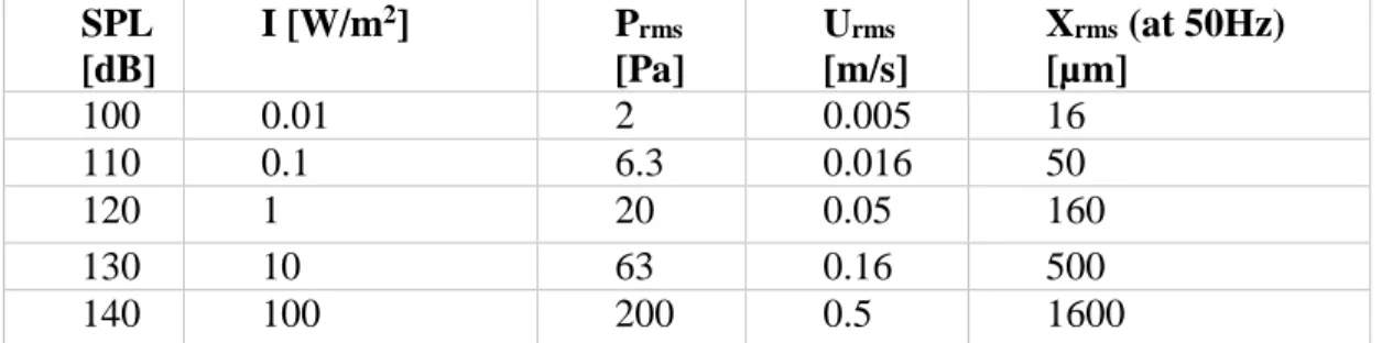
22 SPL [dB] I [W/m2_] _P rms [Pa] Urms [m/s] Xrms (at 50Hz) [µm] 100 0.01 2 0.005 16 110 0.1 6.3 0.016 50 120 1 20 0.05 160 130 10 63 0.16 500 140 100 200 0.5 1600

Table 2.1. Acoustic parameters of a generalized noise source at 100-140 dB SPL.

approximately 100-140 dB SPL. Based on the linearized physics model, this gives rise to acoustic parameters as seen in in Table 2.1.

As measured at a distance of 1000 feet, a typical frequency spectrum from a jet airplane is given in Figure 2.1. This power spectral density provides information on total sound pressure level contained within each frequency bin, with bin centers denoted by data markers.

(23)

23

Bins are defined logarithmically, with centers on third-octave bands, as per industry standard. Most notably, the noise is broadband in nature regardless of aircraft type, with the majority of energy contained below 1000 Hz. Using a Boeing 757-200 as a reference, summation over frequencies yields ~117 dB SPL, or approximately 0.5 W/M2at 1000 feet (330 meters).

2.2 Sound Transducer Technologies

Multiple technologies exist for the transduction of acoustic energy into the electrical domain, and there is significant overlap between acoustic energy harvesting technology and sound sampling technology (microphonics). Several technologies are discussed below. A crucial difference is that in microphonics, a primary design goal is to maximize impedance presented to the source, minimizing loading of the signal and therefore maximizing fidelity and accurate reproduction of the sampled signal. In addition, primary goals include flat frequency response, high linearity, minimization of THD+N (total harmonic distortion plus noise) and optimization for perceived sound quality based on psychoacoustic factors. In contrast, in acoustic energy harvesting the primary goal is to present an impedance which is matched to the source

impedance for maximum energy transfer, with no attention paid to perceived sound quality or related factors.

2.2.1 Electrostatic Transduction

In an electrostatic (condenser) microphone or energy harvester, two conductive plates or diaphragms are separated by a small gap, forming a capacitor [16]. An incoming pressure wave does work against one diaphragm, causing it to move. The diaphragm moves in the presence of an electric field, which is generated by a built-in bias potential (as in large-diaphragm condenser microphones) or a pre-charged electrostatic material (as in electret condenser microphones). The

(24)

24

motion of the diaphragm causes a change in capacitance between the plates. By the principles of electrostatics, a change of capacitance with a fixed charge results in the generation of a time-varying voltage. In a practical electrostatic transducer the parallel plates have a parasitic capacitance which must be modeled and carefully engineered for optimal performance.

2.2.2 Magnetic Transduction

In a magnetic (dynamic) microphone, a diaphragm is caused to move by an incident pressure (sound) wave [16]. In one implementation, the diaphragm contains a coil of wire which moves through a magnetic field produced by static permanent magnets. As described by

Faraday’s law of Induction, the motion of a wire through a magnetic field generates a voltage which by proper electrical design can be extracted as electrical power. In a related

implementation, a diaphragm with an associated magnet moves through a stationary coil,

generating voltage on the same principle. In a practical magnetic transducer, the coil’s resistance and inductance must be modeled and carefully engineered for optimal performance.

2.2.3 Piezoelectric Transduction

In a piezoelectric microphone or energy harvester, a diaphragm is supported by a structure with piezoelectric materials [16]. An incoming pressure wave moves the diaphragm against the spring force arising from the support structure. As described by the piezoelectric effect, a stress in a piezoelectric material creates a dipole moment, resulting in the generation of charge which is extracted as electrical energy or signal. In a practical piezoelectric transducer, the material’s capacitance affects the electromechanical properties of the system, and must be modeled and carefully engineered for optimal performance.

(25)

25

2.2.4 Triboelectric Transduction

Triboelectric transduction is an emerging technology in energy harvesting. As described by the triboelectric effect, two dissimilar materials generate an electric charge (static electricity) upon contact. This effect has been demonstrated to have potential in energy harvesting. In this implementation, an incoming pressure wave moves a diaphragm, causing the repeated contact and separation of two materials, resulting in the constant generation of triboelectric charge which is extracted as electrical energy.

2.2.5 Optimal Transduction for Acoustic Energy Harvesting

A crucial commonality between the transduction technologies named above is

reversibility. A force causes the generation of electrical energy, but the effects can be applied in reverse, applying electrical energy to produce a force. This effect will be exploited in designing a broadband energy harvester, as described in future sections.

While in theory the various transduction technologies equivalently transduce acoustic energy into electrical energy, they differ in implementation and tradeoffs associated with a practical design. As will be discussed in Section 2.5, an optimal broadband acoustic energy harvesting system can be created using a broadband impedance match between the acoustic impedance of air and that of the harvester. Due to the practicalities of building a real acoustic system, this generally involves construction of negative reactive circuit components. As an equivalent statement, the harvester is loaded with an electrical system to provide a frequency-dependent force to the harvester, which counteracts frequency-frequency-dependent forces inherent in the harvester to provide a broadband impedance match.

(26)

26

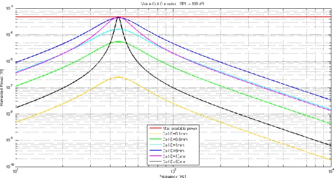
Figure 2.2. Harvested power versus frequency for different coil diameters for a square 10x10cm magnetic harvester with resonant frequency of 500Hz and 100 dB SPL input energy.

As discussed in Section 2.2.2, a magnetic harvester is made by a diaphragm with a coil of wire, which is acted upon by an acoustic force to move through a magnetic field, producing a current. The magnetic field is produced by a stationary magnet. To investigate the feasibility of such an approach for acoustic energy harvesting, an electromechanical circuit model was derived for a generic magnetic harvester based on principles discussed in Section 2.4. The details of this model and simulation code are presented in Appendix A. A key design decision is the gauge of wire and number of turns used in the coil. An inherent tradeoff exists between coil mass and coil resistance. An increase in wire diameter reduces resistance at the expense of increased mass. The increased mass requires more current through the coil for an optimal impedance match. The losses associated with increased current counteract the energy savings from reduced coil

(27)

27

resistance. This tradeoff is seen graphically in Figure 2.2. Even with an optimal coil diameter, optimal broadband harvesting cannot be achieved in this implementation.

An electrostatic harvester is constructed as discussed in Section 2.2.1. As in the magnetic harvester, an electrostatic harvester requires an electronic load to apply a force to the harvester for a broadband impedance match. It can be shown that the pressure applied to an electrostatic energy harvester takes the form

𝑃

_e

=

𝜖𝑉_2𝑑2₂

(2.4)

with Pressure Pe in Pascals, dielectric constant ε in Farads/meter, Voltage V, and distance

between plates d in meters. It can be shown that excessively high voltages are required to produce the electric fields necessary for impedance matching and therefore efficient energy harvesting. As an example from Table 2.1, 110 dB sound at 50 Hz requires a displacement of 50 um rms and a pressure of 6.3 Pa rms. Substituting into (2.4), this yields a required voltage of nearly 10kV, much too high for practical implementations. Thus, electrostatic transduction was deemed impractical for this application.

Triboelectric transduction is based on the mechanism of repeated contact and separation of two materials. Such contact and separation at a displacement of 50 um applies severe

constraints on the mechanical design of the system, making this approach impractical.

Piezoelectric transduction was chosen primarily because of it’s low loss properties and low cost. Furthermore, piezoelectric polymer film of Polyvinylidiene Fluoride was chosen in favor of piezoelectric ceramics such as PZT due to it’s low weight, tunable compliance, low losses and low cost.

(28)

28

2.3 Diffraction Effects

One design issue that is common to acoustic energy harvesters and microphones is that of diffraction. At audio frequencies, wavelengths are typically much longer than transducer

geometries. For example, the wavelength of an acoustic wave at 1KHz is approximately 30cm. As seen in Figure 2.3 below, a consequence of this is that the transducer looks “small” to the incoming wave, and the incoming wave diffracts around the transducer. The transducer is often thin enough that the incoming wave experiences little phase shift from the front to the back of the transducer. A negative consequence of this is that the incoming pressure wave will exert an equal pressure on both sides of the transducer diaphragm, resulting in zero force on the

diaphragm and therefore no energy transfer. Solutions to this issue will be discussed in future sections.

(29)

29

2.4 Acoustic System Modeling

Powerful analytical tools exist which allow for rapid and intuitive modeling of the behavior of such systems. The most commonly used tool is the circuit analogy, which models an acoustic system as an electrical system. Such a model enables the simulation of acoustic systems by numerical simulation software such as SPICE. In addition, it allows acoustic systems to be analyzed using classical circuit techniques such as superposition, sinusoidal steady state analysis and pole-zero analysis. This chapter focuses on the lumped-element circuit analogy technique for acoustic systems.

2.4.1 Lumped Element Approximations

The quasistatic approximation is required to enable acoustic systems to be represented as lumped-element circuit models with reasonable accuracy. This quasistatic approximation has an analogous assumption in electrical circuit systems. In an acoustic system, the quasistatic

approximation assumes that the geometries of an acoustic system are much smaller than the wavelength of the acoustic waves which are interacting with the system, in the axis of wave propagation. A consequence of this is approximation is the approximation that pressure is constant over distance, and that velocity varies linearly with distance. This is seen in Figure 2.4 [1]. This approximation allows transmission line effects to be ignored, and the “lumping” of distributed attributes into idealized components. Such an approximation is also used in circuit modeling, when the circuit’s geometries are much smaller than the electromagnetic wavelengths which are incident on the system. In an acoustic system, the quasistatic approximation can be made with little error when the system’s geometries are much smaller than the incident waves. The relationship between frequency and wavelength of an acoustic wave is given by

(30)

30

Figure 2.4. The quasistatic regime applies for structures much smaller than the wavelengths of interest [1].

𝐶

₀

= 𝑓 ∗ 𝜆

(2.5)

where C0 is 334 meters/second at standard temperature and pressure, frequency f in Hz and

wavelength λ in meters. A few representative examples of frequency and wavelength are given in Table 2.2. Because the harvester is designed to be much smaller than the wavelengths associated with the frequencies of interest (50Hz to 1KHz), the quasistatic approximation is valid for the modeling of this system. Corrections to this approximation are presented in Section 3.7.

Frequency (Hz) Wavelength (m)

10 34.3

100 3.43

1k 0.343

10k 0.034

Table 2.2. Various frequencies and wavelengths of sound in air at standard temperature and pressure, with C0=343 m/s.

(31)

31

The second approximation is that of linearity. While not required for lumped element modeling of an acoustic system, it allows for modeling of the system with standard linear

electrical components. Air is a nonlinear medium, however it can be approximated as linear via a first order Taylor approximation for “small signal” sound levels, when particle velocity’s

magnitude |U| is much less than the speed of sound CO in the medium. For sound levels and

frequencies typical of human hearing, the linear approximation can be made with negligible error [26].

Two distinct models can be applied for modeling acoustic systems as lumped-element circuit models: the impedance analogy and the mobility analogy. This chapter will first focus on the impedance analogy then make the extension to the mobility analogy.

2.4.2 Force Source as Voltage Source

In the impedance analogy model, pressure is modeled as an “across variable”, with units of Pascals, or Newtons per square meter [1]. This is analogous to voltage in an electrical system. Consequently, a pressure source is analogous to an electrical voltage source. In mechanical systems this is often instead represented as force (Newtons), which is simply pressure multiplied by area.

2.4.3 Velocity Source as Current Source

In the impedance analogy model, volume velocity is modeled as a “through variable”, with units of cubic meters per second. This is analogous to current in an electrical system. Consequently, a volume velocity source is analogous to a current source. In mechanical systems the through variable is often instead represented as velocity (meters per second), which is simply volume velocity divided by area. In this case, voltage is analogous to force.

(32)

32

2.4.4 Loss as Resistor

In the impedance analogy model, a real loss can be modeled as an electrical resistor. In a mechanical or acoustic system, real losses can come from effects such as friction and viscous losses. In acoustic systems, such a resistance has units of Pascals/meters3/second. In mechanical systems with force and velocity as across and through variables, a loss resistor model has units of Newtons/meters/second.

2.4.5 Compliance as Capacitor

In the impedance analogy model, a compliance element can be modeled as an electrical capacitor [1]. This can be seen by the relation between a compliance’s pressure and volume velocity

𝑢(𝑡) = 𝐶

_A 𝑑𝑝(𝑡)_𝑑𝑡

(2.6)

where CA is acoustic compliance, given in m3 / Pa. This can be seen as a conservation of mass

statement. In an equivalent electrical model of a mechanical system, a similar relation holds between force and velocity and is given by

𝑣(𝑡) = 𝐶

_M𝑑𝑓(𝑡)_𝑑𝑡

(2.7)

where CM is mechanical compliance, given in meters/newton.

2.4.6 Mass as Inductor

In the impedance analogy model, an acoustic mass element can be modeled as an electrical inductor. This can be seen by the relation between pressure and volume velocity [1]:

(33)

33

𝑢(𝑡) =

_𝐿1

A

∫ 𝑝(𝑡)𝑑𝑡 (2.8)

where LA is acoustic mass, given in Pa*s2/m3. This can be seen as a conservation of momentum

statement. In an equivalent electrical model of a mechanical system, a similar relation holds between force and velocity:

𝑣(𝑡) =

_𝐿1

M

∫ 𝑓(𝑡)𝑑𝑡 (2.9)

where LM is mechanical mass, given in newtons*second2/meters.

A summary of the impedance analogy for both acoustic and mechanical systems is shown in Figure 2.5 [1].

(34)

34

2.4.7 Mechanical to Mechanical Transformers as Electrical

Transformers

Various acoustic structures exist which exhibit a lossless transformation between volume velocity and pressure. Two such examples are horns and pistons, as seen in Figure 2.6. [2].

Such structures maintain energy conservation, while trading pressure for volume velocity or vice-versa. Consequently they have the effect of transforming the acoustic impedance seen at their input terminals. Such a structure can be modeled electrically as a transformer. The windings ratio T is given by

𝑇 =

𝑈2 𝑈₁

=

𝑃₁ 𝑃₂

=

𝐴𝑟𝑒𝑎₂ 𝐴𝑟𝑒𝑎₁

(2.10)

where U1 and U2 are the respective input and output volume velocities, P1 and P2 are the

Figure 2.6. Horn (top) and piston (bottom) structures are analogous to electrical transformers, with windings ratio analogous to area ratio [2].

(35)

35

respective input and output pressures, and Area1 and Area2 are the respective input and output

cross sectional areas. A mechanical equivalent of a transformer between force and velocity is a lever arm, which will not be discussed in further detail here.

2.4.8 Transducer as Electrical Transformer

The transducers described in Section 2.2 share the commonality that they transduce mechanical energy (force and velocity) into electrical energy (voltage and current). Applying this to the circuit analogy described in Sections 2.4.1-2.4.7, an appropriate model for a transducer is an electrical transformer. Such a transducer converts mechanical through and across variables (velocity and force) to electrical through and across variables (voltage and current), in a reversible manner. The effective windings ratio of such a transformer model is based on

implementation: choice of transduction method, geometries, material properties and other design parameters. Real-world transducers also have various parasitic elements as discussed in Sections 2.2.1-2.2.4. In the impedance analogy, a more formal representation for electromechanical transduction is cross-coupled voltage and current sources, as seen in Figure 2.7.

2.4.9 Mobility Analogy

The mobility analogy is an alternative representation of a lumped-element acoustic model as an electrical circuit, and is reciprocal to the impedance analogy. In the mobility analogy, volume velocity is instead mapped to electrical voltage and pressure is mapped to current [1]. Losses, compliances, and masses are now modeled as parallel resistors, inductors and capacitors, respectively. This is analogous to a dual circuit of an electrical circuit, or a transformation from Thévenin equivalence to Norton equivalence. Impedance analogy and mobility analogy circuit models for a second-order Helmholtz resonator acoustic system are shown in Figure 2.7.

(36)

36

Figure 2.7. Impedance (top) and mobility (bottom) circuit analogies for generic Helmholtz acoustic system with transducer.

2.5 Load Matching for Optimal Energy Harvesting

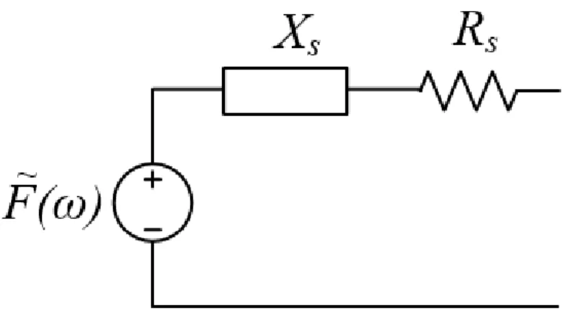
An acoustic system can generally be described by an equivalent circuit model, as seen in Figure 2.7. Using standard linear circuit techniques, this can be described by a Thévenin

equivalent circuit model with a frequency-dependent source and complex source impedance, as seen in Figure 2.8 [3].

A critical insight of this model is that it is electromechanical. It captures both the electrical and mechanical properties of the system. Any mechanical change to the system will

(37)

37

Figure 2.8. Thévenin equivalent circuit model of generic acoustic system, with frequency-dependent voltage source F(ω), reactance Xs and resistance Rs.

manifest as a change in Thévenin impedance seen electrically, and vice-versa. Energy applied to the system mechanically will be seen electrically, and vice-versa. Therefore, mechanical

properties of the system are affected by electrical loading. For example, a reactive loading to the system will change it’s complex impedance characteristic and it’s resonant frequency. This property will be exploited to achieve broadband energy harvesting.

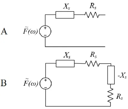
As described by the maximum power transfer theorem [27], a power source with source impedance Zs will transfer the maximum amount of power to a load impedance Zs* which is the complex conjugate of the source impedance, as seen in Figure 2.9b. This concept is widely used in acoustics, electromagnetism, vibration control and many other subfields within electrical and mechanical engineering. For an electromechanical Thévenin equivalent model of an acoustic system as in Figure 2.8, this optimal load is realized as a matched real part Rs and a negated reactive part Xs, as seen in Figure 2.9b.

(38)

38

Figure 2.9. (a) Maximum power transfer is achieved to a load impedance which is the complex conjugate of the source impedance. (b) Such a match is realized with a matched real part and a negative reactive part.

Traditionally such a load is realized at a single frequency using a positive reactive component such as inductance (to match reactance of a capacitor) and capacitance (to match reactance of an inductor). However, such an approach yields narrowband response, which has little utility in energy harvesting applications where input energy is broadband. This technique is widely used in Power Factor Correction circuits, where impedance match is only required at a single frequency [15]. A similarly matched load can also be realized using a negative reactive component. For example, matching an inductive source with a negative inductive load. This has the advantage of matching impedance at all frequencies, allowing for broadband response. However it introduces a number of challenges, including sensitivity and stability, which will be discussed in Sections 5.2 and 5.4, respectively.

(39)

39

2.6 Existing Acoustic Energy Harvesting Approaches

A common approach to acoustic energy harvesting is founded upon the use of a

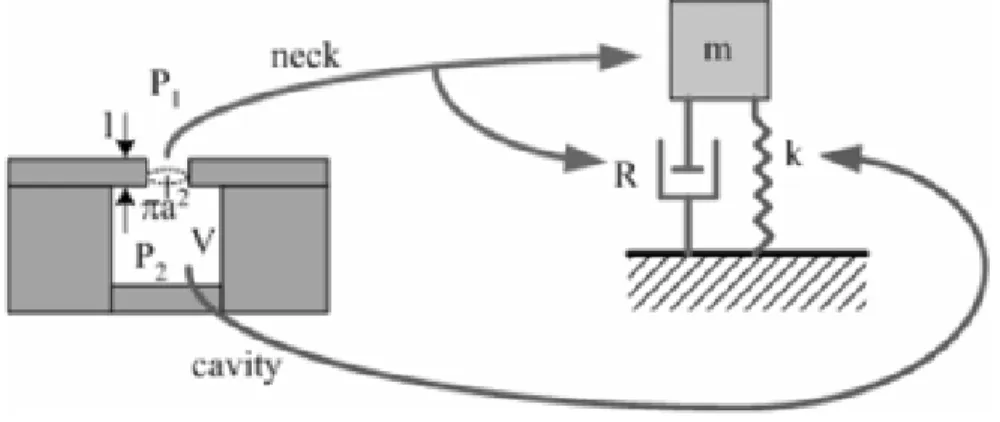
Helmholtz resonator [4]. As seen in Figure 2.10, a Helmholtz resonator is a hollow cavity with a narrow neck, which receives an incident sound wave. Typically, a backplate acts as a diaphragm which moves in a force field in an implementation of one of the transduction technologies described previously. A Helmholtz resonator can be modeled as a second order system, analogous to a RLC circuit system or mass-spring-dashpot system as seen in Figure 2.10 [5].

An advantage of this approach is that minimal damping can result in very high Q, or very highly resonant systems. The Q amplification provided by this resonance can result in highly efficient energy transfer at the resonant frequency due to mechanical systems having generally smaller forces and large motions. However, a significant drawback of this approach is that a high Q results in a very narrow bandwidth, significantly limiting the frequencies over which the harvester can efficiently harvest energy. This approach still has application in areas where the

(40)

40

noise source is fixed at a known frequency. However, it has low efficiency for noise sources which are broadband or varying in frequency, such as aircraft noise.

Multiple approaches [6] have been proposed for increasing the frequency range of energy harvesters, or allowing harvesting frequency to be tunable. Phipps et al [7] has demonstrated a system with multiple energy harvesters in parallel, each having a slightly different resonant frequency. This system has the appearance of a broadband system. However, it has the drawback of being space inefficient, with very few of the many harvesters collecting energy efficiently at any given time. Williams et al [8] describes a system with a reduced Q factor (increased

dampening). While this does increase the frequency range of collection, it comes at the expense of decreasing collection efficiency at any one frequency.

Many sources have described achieving tunable harvesting by the use of variable-length cantilevers or variable spring tension [6]. While this approach allows for tunable resonant frequency, the downside of narrow bandwidth remains. A coupled oscillator effect with a higher-order system has been described by Petroupolos et al [9], however it also demonstrated reduced efficiency than a generator with a single mass. Amplitude limitation and nonlinear effects have been described variously in the literature [6]. These devices work generally by exploiting a nonlinearity in the system, allowing the resonant frequency to be changed with manipulation of system operating point. These devices typically show increased bandwidth over a variable range of frequencies and often are sensitive to the direction of frequency variation. Thus, they are unable to collect energy from arbitrary frequency/time combinations and as such are not truly broadband.

Multiple sources [10] [11] have reported the use of variable load impedance to enable a tunable harvester. These systems generally exploit the reversible nature of the transducer to

(41)

41

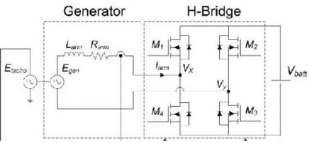
Figure 2.11. A full-bridge switching rectifier for tunable load impedance.

manipulate the reactance of the mechanical system by variation of reactance in an electrical load. Mallick et al [12] demonstrates the variation of resonant frequency by variation in load

capacitance. This approach has been extended by the use of switching power electronics to synthesize reactance, as reported by Kaphengst et al [10], and also Chang et al [11]. In this approach, an electrically controllable H bridge active rectifier is used in lieu of a standard full-bridge diode rectifier as seen in Figure 2.11, in a similar approach to that used in active power factor correction circuitry [15].

By sensing source voltage and load current and addition of a classical control scheme, the active rectifier can be controlled to synthesize negative electrical reactances to interact with mechanical reactances in order to tune the resonant frequency electrically. This approach has also been used to create a harvesting system with multiple resonant frequencies, as described by Chang et al [11]. It is this approach that will be extended in this work to create a truly broadband energy harvester.

(42)

42 Figure 2.12. A MEMS-scale acoustic energy harvester.

Figure 2.13. A Magnetic acoustic energy harvester.

Another notable commonality between existing energy harvesters is their size. The

majority of harvesters reported in literature are either micro-scale based on MEMS techniques, or very large scale vibration harvesters for ocean wave-based applications. Existing MEMS

harvesters tend to have collection areas of fractions of a square centimeter, with correspondingly small power output levels. For example, Horowitz et al [5] reports a nano-scale harvester based on Silicon-on-Insulator techniques with a collection area of 17.4mm2_{, as seen in Figure 2.12.}

(43)

43

Kim et al [13] report a slightly larger collector based on magnetic transduction, as seen in Figure 2.13.

The generally diminutive size coupled with the limitation of narrow band energy

harvesting limit existing acoustic energy harvesters to very low power output levels, on the order of nanowatts to microwatts. On the opposite end are large-scale harvesters intended for marine wave applications [17]. Little research attention has been directed towards energy scales between these two extremes, such as energy scales appropriate for wireless sensor node applications. Thus, a significant opportunity exists to innovate and improve upon acoustic energy harvester technology, both by increasing frequency range and improving upon size. The improvement of output power would enable the use of acoustic energy harvesters in wireless remote sensor node or similar applications.

The use of PVDF and negative capacitance circuits has been explored in the context of noise isolation. Sluka et al [18] describe a curved PVDF film loaded with a negative capacitance generated by an operational amplifier circuit. Broadband performance is limited by their inability to match the load with the dependent capacitance PVDF arising from it’s frequency-dependent dielectric constant. Various authors [18] [19] also describe a dynamic circuit with feedback control to optimize the load negative capacitance value. Date et al [20] provides the initial theoretical analysis of the PVDF/negative capacitance approach, and describes an extreme sensitivity to load capacitance, which requires a ~0.1% precision. Fukada et al [21] describe tunable narrowband sound isolation using a negative capacitance load. Kim et al [22] describe a successful broadband sound isolation system using two pieces of curved PVDF film and a negative capacitance circuit. Crucially, the above literature uses piezoelectric PVDF film with negative capacitance load to increase effective stiffness of the system, providing a sound

(44)

44

isolation effect by reflecting incident sound. In such systems no energy is extracted from the sound and impedance of the load is maximized rather than matched to the source. No precedent was found literature for the use of PVDF and negative capacitance for acoustic energy

harvesting. There was similarly no precedent found for demonstration of similarly large-scale or broadband acoustic energy harvesting.

2.7 Chapter Summary

Energy exists in the air particle motion associated with sound. The energy is a square function of sound pressure, and an inverse square function of distance from noise source. It is linearly related to collection area. Various technologies exist for transduction between acoustic and electrical energy, many of which are used in microphonics. Piezoelectric transduction has been identified as the optimal transduction technology due to it’s low parasitic properties.

Powerful analytical models exist for the modeling of acoustic or mechanical systems as electrical circuits, allowing them to be analyzed by classical circuit techniques such as Thévenin and Norton equivalence and superposition. Such techniques are used for realizing an efficient

broadband acoustic energy harvester by matching the source impedance of an electromechanical system with a matched conjugate electrical load. This concept has been explored in the context of sound isolation by the use of piezoelectric PVDF transducers and negative capacitance circuits. Existing acoustic energy harvesting technologies are limited in performance due to diminutive size and lack of efficient broadband harvesting. A piezoelectric film transducer is used for energy harvesting, and the use of negative reactive components are employed for efficient broadband energy harvesting.

(45)

45

Chapter 3 Acoustic Energy Harvester Analysis and

Model

This chapter develops an analytical model, describing electromechanical dynamics of the above acoustic energy harvester. The end result is a lumped-element circuit model of a

distributed system describing the harvester’s mechanical, transduction, and electrical properties. The model is lumped on a modal basis, considering only the first mode of film behavior. This model is instrumental in developing appropriate load circuitry for efficient broadband energy harvesting. The model is then validated experimentally, as described in future sections. The base dynamics model is based on an energy conservation statement. This is later extended to include second-order effects, such as back-cavity reflections.

The total system energy is the sum of energy contributions from kinetic energy, strain energy, and electric field energy. Thus,

In the energy analysis, the derivative of system energy equals net power into or out of the system as expressed by

𝐸

_{system, total}

= 𝐸

_kinetic

+ 𝐸

_strain

+ 𝐸

_{E field}

(3.1)

𝑑

(46)

46

Figure 3.1. Assumed mode shape of PVDF film energy harvester, side view. Length L given in meters and maximum film displacement A0 also given in meters.

where Pin and Pout are input and output powers, respectively. This can be seen as a conservation of energy statement. Expansion of (3.2) then yields the desired dynamic model.

The analysis begins by examining a square film of piezoelectric PVDF film, and assuming a film shape with only a fundamental mode in each dimension as seen in Figure 3.1. The mode shape is assumed to be

with L as length of the film (meters) in dimensions x and y, and A0 the peak modal film

displacement for the film’s fundamental mode, given in meters.

3.1 Kinetic Energy: Effective Mass M

Kinetic energy of the film is derived by integrating kinetic energy over small volumes of film with dimensions dx,dy. Thus,

𝐴(𝑥, 𝑦, 𝑡) = 𝐴

_𝑜

(𝑡) sin (

𝜋𝑥

𝐿

) sin(

𝜋𝑦

(47)

47

𝐸

_kinetic

= ∫ ∫

₀𝐿 ₀𝐿1₂

𝜌𝑇 (

𝑑𝐴_𝑑𝑡

)

2

𝑑𝑦𝑑𝑥 (3.4)

with film mass density ρ (Kg/m3_{), and thickness T (meters). Substitution of (3.3) into (3.4)}

evaluates to

𝐸

_kinetic

=

𝜌𝑇𝐿₈ 2

(

𝑑𝐴0

𝑑𝑡

)

2

(3.5)

The power arising from kinetic energy can be evaluated by taking the time derivative of kinetic energy 𝑑𝐴_𝑜 𝑑𝑡

𝐹

mass

=

𝑑 𝑑𝑡

(𝐸

kinetic

) =

𝑑 𝑑𝑡

(

𝜌𝑇𝐿2 8

(

𝑑𝐴₀ 𝑑𝑡

)

2

) =

𝜌𝑇𝐿2 4 𝑑2𝐴₀ 𝑑𝑡2 𝑑𝐴_𝑜 𝑑𝑡

(3.6)

Therefore, the fundamental mode’s effective mass M (kilograms) can be seen by inspection as

𝑀 =

𝜌𝑇𝐿₄ 2

(3.7)

3.2 Strain Energy: Spring Coefficient K

Based on the assumed film shape in (3.3), spatial derivatives are evaluated as

𝑑𝐴 𝑑𝑥

= 𝐴

0

(𝑡)

𝜋 𝐿

cos (

𝜋𝑥 𝐿

) sin (

𝜋𝑦 𝐿

) (3.8)

𝑑𝐴 𝑑𝑦

= 𝐴

0

(𝑡)

𝜋 𝐿

sin (

𝜋𝑥 𝐿

) cos (

𝜋𝑦 𝐿

) (3.9)

(48)

48 𝑑𝐴 𝑑𝑡

=

𝑑𝐴₀(𝑡) 𝑑𝑡

sin (

𝜋𝑥 𝐿

) sin (

𝜋𝑦 𝐿

)

(3.10)

Strain in x and y are evaluated by integrating over the length of the film, yielding

𝜖

_𝑥

(𝑦, 𝑡) =

1_𝐿

∫ √1 + (

₀𝐿 𝑑𝐴_𝑑𝑥

)

2

𝑑𝑥 − 1

(3.11)

𝜖

_𝑦

(𝑥, 𝑡) =

1_𝐿

∫ √1 + (

₀𝐿 𝑑𝐴_𝑑𝑦

)

2

𝑑𝑦 − 1

(3.12)

This is approximately equal to

𝜖

_𝑥

(𝑦, 𝑡) ≈

1 𝐿

∫ (1 +

1 2

(

𝑑𝐴 𝑑𝑥

)

2

) 𝑑𝑥 − 1

𝐿 0

(3.13)

𝜖

_𝑦

(𝑥, 𝑡) ≈

1_𝐿

∫ (1 +

₀𝐿 1₂

(

_𝑑𝑦𝑑𝐴

)

2

) 𝑑𝑦 − 1

(3.14)

Substituting (3.8) and (3.9) into (3.13) and (3.14) yields

𝜖

_𝑥

(𝑦, 𝑡) = (

_2𝐿𝜋

)

2

𝐴

2₀

_{(𝑡) sin}

2 𝜋𝑦

𝐿

(3.15)

𝜖

_𝑦

(𝑦, 𝑡) = (

_2𝐿𝜋

)

2

𝐴

₀2

(𝑡) sin

2 𝜋𝑥

𝐿

(3.16)

The stress-strain relationship for a generic bending material is given by (25)

[

_𝜖

𝜖

𝑥 𝑦

] =

1 𝐸

[ 1

−𝜈

1 ] [

𝜎

_𝑥

𝜎

_𝑦

] (3.17)

with Young’s Modulus E (Pa), Poisson’s ratio ν (unitless), and stress in x and y σx and σy (Pa).

(49)

49

[

_𝜎

𝜎

𝑥 𝑦

] =

𝐸 1−𝑣2

[1 𝜈

𝜈 1

] [

𝜖

_𝑥

𝜖

_𝑦

]

(3.18)

The total strain energy in a material is given by integrating energy density over the piezoelectric volume [24]. Doing so yields

𝐸

_strain

= ∫ ∫ ∫ (

1₂

𝜎

_𝑥

𝜖

_𝑥

+

1 2

𝜎

𝑦

𝜖

𝑦

) 𝑑𝑥𝑑𝑦𝑑𝑧

𝐿 0 𝐿 0 𝑇 0

(3.19)

Substituting (3.15-3.17) into (3.18) and using the result to evaluate the integral in (3.19) yields total strain energy as

𝐸

_strain

=

𝑇𝐸𝐿_8(1−𝜈2(3+2𝜈)₂₎

(

𝜋𝐴𝑜

2𝐿

)

4

(3.20)

The power arising from the stress field is the time derivative of strain energy. Thus,

𝑑𝐴₀ 𝑑𝑡

𝐹

strain

=

𝑑 𝑑𝑡

(𝐸

strain

) =

𝑇𝐸𝐿2(3+2𝜈) 2(1−𝜈2)

(

𝜋 2𝐿

)

4

𝐴

_𝑜3 𝑑𝐴0 𝑑𝑡

(3.21)

This can be understood as a cubic spring, with force being proportional to film displacement cubed. Matching terms to Hooke’s law yields an effective cubic spring constant Kspring as

𝐾

_spring

=

𝑇𝐸𝐿_2(1−𝜈2(3+2𝜈)₂₎

(

_2𝐿𝜋

)

4

(3.22)

where Kspring has units of Newtons/meter3.

At this point, the total forces on the film are a summation from mass and spring forces. Combining (3.21) and (3.6) and evaluating,

(50)

50

𝐹

_total

=

𝑇𝐸𝐿_2(1−𝜈2(3+2𝜈)₂₎

(

_2𝐿𝜋

)

4

𝐴

_𝑜3

+

𝜌𝑇𝐿₄ 2𝑑2𝐴0

𝑑𝑡2

(3.23)

where Ftotal is the total force on the film, in the absence of piezoelectric effects, sources or

damping. This can be seen as an undamped mass-spring system.

3.3 E-Field Energy: Electromechanical Transducer Ratio

D

For piezoelectric materials the stress-strain relationships include an electric field term arising from the piezoelectric effect and are defined as

[

_𝜖

𝜖

𝑥 𝑦

] =

1 𝐸

[ 1

−𝜈

1 ] [

𝜎

_𝑥

𝜎

_𝑦

] + [

𝑑

_𝑑

31₃₂

] 𝐸

𝑧

(3.24)

with piezoelectric coefficients d31 and d32 in x and y dimensions (Coulombs/Newton), and

electric field Ez in the z direction (Volts/Meter).

In a piezoelectric material, electric displacement Dz (C/m2) is given by

𝐷

_𝑧

= [𝑑

31

𝑑

31

] [

𝜎

_𝑥

𝜎

_𝑦

] + 𝜖𝐸

𝑧

(3.25)

where 𝜖 is the dielectric constant of the piezoelectric material (Farads/meter). Stress in x and y, σx and σy,can be found by rearranging (3.24) to obtain

[

_𝜎

𝜎

𝑥 𝑦

] =

𝐸 1−𝑣2

[1 𝜈

_{𝜈 1}

] [

𝜖

_𝑥

𝜖

_𝑦

] +

1−𝑣𝐸 2

[1 𝜈

_{𝜈 1}

] [

𝑑

₃₁

𝑑

₃₂

] 𝐸

𝑧

(3.26)

(51)

51

Substituting (3.15), (3.16), and (3.26) into (3.25) yields Dz as a function of x and y, according to

𝐷

_𝑧

=

𝑑31𝐸 1−𝜈

(

𝜋 2𝐿

)

2

𝐴

2₀

_{(𝑡) (sin}

2 𝜋𝑥 𝐿

+ sin

2 𝜋𝑦 𝐿

) + 𝐸

𝑧

(𝜖 −

2𝑑₃₁2 𝐸 1−𝑣

) (3.27)

The electric field in the z direction is a function of voltage V over film thickness such that

𝐸

_𝑧

=

𝑉

𝑇

(3.28)

Charge Q in Coulombs can be found by integration of the electric displacement Dz over piezoelectric film surface, as described by Gauss’s Law, to obtain

𝑄 = ∫ ∫ 𝐷

₀𝐿 ₀𝐿 𝑧

𝑑𝑥𝑑𝑦

(3.29)

Substituting (3.27) and (3.28) into (3.29) and evaluating yields

𝑄 =

𝐿2𝑉 𝑇

(𝜖

3

−

2𝐸𝑑₃₁2 1−𝑣

) +

𝐴_𝑜2𝐸𝑑₃₁𝜋2 4(1−𝑣)

(3.30)

which can be seen as an expression for the total charge Q on the piezoelectric film.

In an open-circuit condition, the net external charge is zero. Therefore, the following expression results: 𝐿2𝑉 𝑇

(𝜖

3

−

2𝐸𝑑₃₁2 1−𝑣

) = −

𝐴_𝑜2𝐸𝑑₃₁𝜋2 4(1−𝑣)

(3.31)

(52)

52

This can be seen by inspection as two terms: a contribution from film deflection Ao arising from the piezoelectric effect, and an effective capacitance arising from the film’s dielectric behavior. Differentiating the mechanical contribution with respect to A yields

𝐷 =

_𝑑𝐴𝑑 𝑜

(

𝐴_𝑜2𝐸𝑑₃₁𝜋2 4(1−𝑣)

) =

𝐴_𝑜𝐸𝑑₃₁𝜋2 2(1−𝑣)

(3.32)

where D is the electromechanical transduction ratio between current and velocity.

3.4 E-Field Energy: Effective Capacitance C

Effective capacitance C can be seen by matching the voltage term in (3.30) to capacitive behavior Q=CV. By inspection, effective capacitance C (farads) is equal to

𝐶 =

𝐿2

𝑇

(𝜖

3

−

2𝐸𝑑₃₁2

1−𝑣

)

(3.33)

The energy contribution arising from the electric field is equal to

𝐸

_{E Field}

=

1 2

𝐶𝑉

2

₌

1 2 𝐿2 𝑇

(𝜖

3

−

2𝐸𝑑₃₁2 1−𝑣

) 𝑉

2

_(3.34)

3.5 Input Power: Damping B

The damping factor B arises from energy lost to the system due to reflections of the incoming pressure wave off the piezoelectric film. This can be seen by a force balance assertion applied to the film, assuming incoming acoustic wave of pressure p+ and particle velocity u+,

reflected acoustic wave of pressure p- and particle velocity u-, transmitted acoustic wave of

pressure q+ and velocity v+, and film velocity and pressure defined respectively by U and P, as

(53)

53

Figure 3.2. Incoming, reflected and transmitted particle velocity and pressure waves, and velocity and force arising from the film.

Conservation of mass on both sides of the film set relationships between incoming, reflected and transmitted particle velocity as

𝑈 = 𝑣

₊

(3.35)

𝑈 = 𝑢

₊

+ 𝑢

₋

(3.36)

The net pressure P across the film is described by the incoming, reflected and transmitted pressure waves as

𝑃 = 𝑝

₊

+ 𝑝

₋

− 𝑞

₊

(3.37)

Applying (3.35), (3.36), (3.37) and (2.3), the net pressure evaluates to

𝑃 = 2𝑍

₀

(𝑢

₊

− 𝑈)

(3.38)

The instantaneous incoming power is evaluated as the product of pressure and velocity, integrated over the film area:

(54)

54

𝑃𝑜𝑤𝑒𝑟

_in

= ∫ ∫ 𝑃𝑈 𝑑𝑥𝑑𝑦

₀𝐿 ₀𝐿

(3.39)

Applying (3.38), (3.39), and (3.10) and evaluating, incoming power can be expressed as

𝑃𝑜𝑤𝑒𝑟

_in

=

𝑑𝐴𝑜 𝑑𝑡

𝐹 = 2𝑍

0

𝑢

+

(

2𝐿 𝜋

)

2 𝑑𝐴_𝑜 𝑑𝑡

−

𝑍₀𝐿2 2

(

𝑑𝐴_𝑜 𝑑𝑡

)

2

(3.40)

This can be seen to have two contributions to system net power input/output: a power input arising from the incoming pressure wave, and a power output (loss, dampening term) arising from reflection and radiation of acoustic waves. By inspection, the damping term B can be fit to the classical damping model F=BdAo/dt as

𝐵 =

𝑍0𝐿2

2

(3.41)

3.6 Input Power: Source F

The input power source F can be seen from the net system power input/output in expression (3.40). By inspection, the term arising from the incoming pressure wave is:

𝐹 = 2𝑍

₀

𝑢

₊

(

2𝐿

𝜋

)

2

= (

8𝐿2

𝜋2

) 𝑝

+

(3.42)

It is noted that in this harvester design, it is impossible to harvest all incoming energy incident on the harvester. This is due to the film’s constrained boundaries, which prevent the film from displacing equally over the entire film area. Due to this, energy cannot be optimally extracted over the entire film area simultaneously. As a result, the maximum efficiency possible with this harvester design is 64/(π)4_{, or approximately 66%. This distributed parameter is captured in the}

(55)

55

3.7 Transmission Line: Back-cavity effect

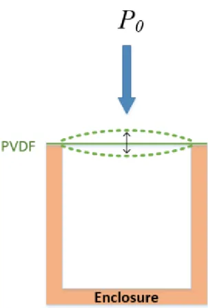
To address performance degradation associated with diffraction effects as discussed in Section 2.3, the piezoelectric PVDF film is supported with an enclosure on one side, creating a cavity as seen in Figure 3.3. A constant pressure inside the cavity provides a pressure reference point for acoustic forces acting on the film.

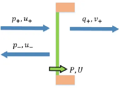
The back cavity also applies a force on the harvester film due to acoustic waves launched by the film’s motion reflected at the rear of the cavity, and interacting with the film. The analysis is performed assuming a one-dimensional transmission line, similar to classical quarter-wave resonators. Consider the film and enclosure system as a transmission line of length Δ (meters), as

Figure 3.3. The harvester is enclosed, addressing performance loss associated with diffraction effects.

(56)

56

Figure 3.4. Film with velocity U and pressure P. Back cavity of length D. Launched pressure and velocity waves p+ and u+, and reflected pressure and velocity waves p- and u-.

seen in Figure 3.4. The film’s velocity and pressure are given as U and P, respectively. Launched pressure and velocity waves are given as p+ and u+, respectively. Reflected pressure and velocity

waves are given as p- and u-, respectively.

Pressure and velocity waves are expressed in time-harmonic form as

𝑢

₊

= 𝑢̂

₊

𝑒

𝑗(𝜔𝑡−𝑘𝑥)

(3.43)

𝑢

₋

= 𝑢̂

₋

𝑒

𝑗(𝜔𝑡+𝑘𝑥)

(3.44)

𝑝

₊

= 𝑍

_𝑜

𝑢̂

₊

𝑒

𝑗(𝜔𝑡−𝑘𝑥)

(3.45)

Broadband acoustic energy harvesting via synthesized electrical loading