Constraining nucleation, condensation, and chemistry
in oxidation flow reactors using size-distribution
measurements and aerosol microphysical modeling
The MIT Faculty has made this article openly available.
Please share
how this access benefits you. Your story matters.
Citation
Hodshire, Anna L., Brett B. Palm, M. Lizabeth Alexander, Qijing
Bian, Pedro Campuzano-Jost, Eben S. Cross, Douglas A. Day, et al.
“Constraining Nucleation, Condensation, and Chemistry in Oxidation
Flow Reactors Using Size-Distribution Measurements and Aerosol
Microphysical Modeling.” Atmospheric Chemistry and Physics 18,
no. 16 (August 28, 2018): 12433–12460.
As Published
http://dx.doi.org/10.5194/acp-18-12433-2018
Publisher
Copernicus Publications
Version
Final published version
Citable link
http://hdl.handle.net/1721.1/118751
Terms of Use
Creative Commons Attribution 4.0 International License
https://doi.org/10.5194/acp-18-12433-2018 © Author(s) 2018. This work is distributed under the Creative Commons Attribution 4.0 License.
Constraining nucleation, condensation, and chemistry in oxidation
flow reactors using size-distribution measurements
and aerosol microphysical modeling
Anna L. Hodshire1, Brett B. Palm2,a, M. Lizabeth Alexander3, Qijing Bian1, Pedro Campuzano-Jost2, Eben S. Cross4,b, Douglas A. Day2, Suzane S. de Sá5, Alex B. Guenther6,7, Armin Hansel8, James F. Hunter4, Werner Jud8,c, Thomas Karl9, Saewung Kim6, Jesse H. Kroll3,10, Jeong-Hoo Park11,d, Zhe Peng2, Roger Seco6, James N. Smith12, Jose L. Jimenez2, and Jeffrey R. Pierce1
1Department of Atmospheric Science, Colorado State University, Fort Collins, CO 80523, USA 2Dept. of Chemistry and Cooperative Institute for Research in Environmental Sciences (CIRES), University of Colorado, Boulder, CO 80309, USA
3Environmental and Molecular Sciences Laboratory, Pacific Northwest National Laboratory, Richland, WA 99352, USA 4Department of Civil and Environmental Engineering, Massachusetts Institute of Technology, Cambridge, MA 02139, USA 5School of Engineering and Applied Sciences, Harvard University, Cambridge, MA 02138, USA
6Department of Earth System Science, University of California, Irvine, Irvine, CA 92697, USA
7Division of Atmospheric Sciences & Global Change, Pacific Northwest National Laboratory, Richland, WA 99352, USA 8Institute of Ion and Applied Physics, University of Innsbruck, Innsbruck, 6020, Austria
9Institute for Atmospheric and Cryospheric Sciences, University of Innsbruck, Innsbruck, 6020, Austria 10Department of Chemical Engineering, Massachusetts Institute of Technology, Cambridge, MA 02139, USA 11National Center for Atmospheric Research, Boulder, CO 80305, USA
12Department of Chemistry, University of California, Irvine, CA 92697, USA
anow at: Department of Atmospheric Sciences, University of Washington, Seattle, WA 98195, USA bnow at: Center for Aerosol and Cloud Chemistry, Aerodyne Research, Inc., Billerica, MA 01821, USA cnow at: Institute of Biochemical Plant Pathology, Research Unit Environmental Simulation,
Helmholtz Zentrum München, Munich, 85764, Germany
dnow at: Climate and Air Quality Research Department, National Institute of Environmental Research (NIER), Incheon, 22689, Republic of Korea
Correspondence: Anna L. Hodshire (hodshire@rams.colostate.edu)
Received: 2 March 2018 – Discussion started: 7 May 2018
Revised: 19 July 2018 – Accepted: 17 August 2018 – Published: 28 August 2018
Abstract. Oxidation flow reactors (OFRs) allow the con-centration of a given atmospheric oxidant to be increased beyond ambient levels in order to study secondary organic aerosol (SOA) formation and aging over varying periods of equivalent aging by that oxidant. Previous studies have used these reactors to determine the bulk OA mass and chemical evolution. To our knowledge, no OFR study has focused on the interpretation of the evolving aerosol size distributions. In this study, we use size-distribution measurements of the OFR and an aerosol microphysics model to learn about size-dependent processes in the OFR. Specifically, we use OFR
exposures between 0.09 and 0.9 equivalent days of OH aging from the 2011 BEACHON-RoMBAS and GoAmazon2014/5 field campaigns. We use simulations in the TOMAS (TwO-Moment Aerosol Sectional) microphysics box model to con-strain the following parameters in the OFR: (1) the rate constant of gas-phase functionalization reactions of organic compounds with OH, (2) the rate constant of gas-phase frag-mentation reactions of organic compounds with OH, (3) the reactive uptake coefficient for heterogeneous fragmentation reactions with OH, (4) the nucleation rate constants for three different nucleation schemes, and (5) an effective
accommo-dation coefficient that accounts for possible particle diffusion limitations of particles larger than 60 nm in diameter.
We find the best model-to-measurement agreement when the accommodation coefficient of the larger particles (Dp> 60 nm) was 0.1 or lower (with an accommodation co-efficient of 1 for smaller particles), which suggests a diffu-sion limitation in the larger particles. When using these low accommodation-coefficient values, the model agrees with measurements when using a published H2SO4-organics nu-cleation mechanism and previously published values of rate constants for phase oxidation reactions. Further, gas-phase fragmentation was found to have a significant impact upon the size distribution, and including fragmentation was necessary for accurately simulating the distributions in the OFR. The model was insensitive to the value of the reac-tive uptake coefficient on these aging timescales. Monoter-penes and isoprene could explain 24 %–95 % of the observed change in total volume of aerosol in the OFR, with ambient semivolatile and intermediate-volatility organic compounds (S/IVOCs) appearing to explain the remainder of the change in total volume. These results provide support to the mass-based findings of previous OFR studies, give insight to im-portant size-distribution dynamics in the OFR, and enable the design of future OFR studies focused on new particle forma-tion and/or microphysical processes.
1 Introduction
Aerosols impact the climate directly, through absorbing and scattering incoming solar radiation (Charlson et al., 1992), and indirectly, through modifying cloud properties (Rosen-feld et al., 2008; Clement et al., 2009). Both of these ef-fects are size-dependent, with larger particles dominating both effects. Particles with diameters (Dp) greater than 50– 100 nm can act as cloud condensation nuclei (CCN) and par-ticles with Dpgreater than 200–300 nm can absorb and scat-ter radiation more efficiently than smaller particles (Seinfeld and Pandis, 2006). The radiative forcing predictions of these effects remain amongst the largest uncertainties in climate modeling (Boucher et al., 2013), and thus climate predictions rely greatly upon accurate simulations or assumptions of the particle size distributions. The majority of the aerosol num-ber globally is derived from photochemically driven new-particle formation (NPF) of ∼ 1 nm new-particles (e.g., Spracklen et al., 2008; Pierce and Adams, 2009a). These new particles are too small to impact climate, and they must grow through uptake of vapors and similarly sized particles while avoiding being lost by coagulation to larger particles in order to reach climatically relevant sizes (Westervelt et al., 2014). Thus, ac-curately simulating new particle formation and growth pro-cesses is a key step towards representing particle size dis-tributions and predicting aerosol–climate effects in regional and global models that assess aerosol impacts. In the
fol-lowing paragraphs, we discuss the processes that shape new-particle formation and growth processes relevant to the anal-yses in this paper.
A large fraction of submicron aerosol mass is composed of organic aerosol (OA) (Murphy et al., 2006; Zhang et al., 2007; Jimenez et al., 2009; Shrivistava et al., 2017). OA is composed of thousands of often-unidentified compounds (Goldstein and Galbally, 2007) and can be emitted directly in the particle phase as primary OA (POA) or formed as secondary OA (SOA) through gas-to-particle conversion. In SOA formation through the gas phase, atmospheric oxidants (mainly OH, O3, and NO3) react with organic gases to form either less-volatile functionalized compounds or often more-volatile fragmentation products. If the oxidation products have a low-enough volatility, they may then partition to the particle phase, forming SOA (Pankow, 1994; Donahue et al., 2006). The vapors may either partition to pre-existing particles or form new particles through NPF. Alternatively, the oxidation products could react in the particle phase to form lower volatility products that then remain in the parti-cle phase (e.g., Paulot et al., 2009).
Controlled studies of SOA formation have traditionally used large reaction chambers with residence times of hours (often referred to as “smog chambers”). Chambers are sus-ceptible to loss of both gases and particles to the walls of the chambers (e.g., Krechmer et al., 2016; Bian et al., 2017). In order to enable the study of SOA formation from ambi-ent air and limit wall losses, oxidation flow reactors (OFRs, i.e., the potential aerosol mass (PAM) reactor; Kang et al., 2007; Lambe et al., 2011a) were developed to produce high and controllable oxidant concentrations and have short resi-dence times (usually ∼ 2–4 min), with the purpose of simu-lating hours to days or weeks of equivalent atmospheric ag-ing (eq. days) in either laboratory or field experiments. Wall losses in OFRs can often be smaller than in large chambers due to shorter residence times (e.g., Palm et al., 2016), al-though a direct comparison requires specification of the oper-ating conditions, and losses in both types of reactors are still a subject of research. Studies with OFRs have shown SOA yields from precursor gases are similar to yields from smog chambers (Kang et al., 2007; Lambe et al., 2011b, 2015; Palm et al., 2018). Previous field studies with OFRs have fo-cused on bulk aerosol mass formation and aging, and bulk chemical evolution (e.g., Ortega et al., 2013, 2016; Tkacik et al. 2014; Palm et al., 2016, 2017, 2018). Ortega et al. (2016) and Palm et al. (2016) showed that size distributions in OFR output were dynamic as a function of time and aging. How-ever, to the best of our knowledge, no ambient OFR study has focused on the aerosol size distributions that form and evolve within the OFR. Processes that could help shape the size dis-tribution within the OFR are the same as those that take place in the real atmosphere, and include nucleation, condensation of vapors, coagulation, the rate of gas-phase oxidation with OH, gas-phase fragmentation with OH, vapor uptake and/or particle diffusion limitations, reactive uptake growth
mecha-nisms including accretion reactions and acid–base reactions, heterogeneous reactions, and wall losses of both vapors and particles. Many of these processes have uncertainties asso-ciated with them, necessitating model-to-measurement com-parisons and sensitivity studies. Using an OFR extends the parameter space over which comparisons can be made, com-pared to using only ambient data where parameter variations are narrower.
Nucleation, i.e., the formation of new ∼ 1 nm particles, can involve a number of species, including water, sulfuric acid, ammonia, amines, ions, and certain low-volatility or-ganic compounds (e.g., Kulmala et al., 1998, 2002; Vehka-maki et al., 2002; Napari et al., 2002; Laakso et al., 2002; F. Yu, 2006; F. Q. Yu, 2006; Metzger et al., 2010; Almeida et al., 2013; Jen et al., 2014; Riccobono et al., 2014). Along with multiple species, observations indicate that numerous physical and chemical reactions can be involved (e.g., Zhang et al., 2004; Chen et al., 2012; Almeida et al., 2013; Ric-cobono et al., 2014). Recent studies have pointed to the importance of nucleation involving sulfuric acid and oxy-genated organic compounds over the forested continental boundary layer (BL) (e.g., Metzger et al., 2010; Riccobono et al., 2014). However, controlled nucleation and growth stud-ies in smog chambers or oxidation flow reactors involving organics have traditionally focused on organics formed from the oxidation of a single precursor vapor, such as α-pinene. Previous chamber studies have examined NPF from plant emissions (e.g., Joutsensaari et al., 2005; Vanreken et al., 2006), but to our knowledge no studies have systematically investigated nucleation and growth mechanisms in OFR or other types of reactors using ambient air as the precursor source.
Condensation of vapors to newly formed aerosol particles as well as pre-existing particles increases the total aerosol particle mass, but the net condensation rate to differently sized particles is dependent upon the volatility of the va-pors. The lowest-volatility vapors condense essentially irre-versibly onto particles of all sizes (i.e., “kinetically limited” or irreversible condensation; Riipinen et al., 2011; Zhang et al., 2012). Semi-volatile vapors (with non-trivial partitioning fractions in both the particle and gas phases at equilibrium) have a net condensation to particles that is determined by reversible partitioning (i.e., quasi-equilibrium condensation; Riipinen et al., 2011; Zhang et al., 2012). Kinetically limited condensation is gas-phase-diffusion limited and only possi-ble for compounds with effective saturation concentrations (C∗; Donahue et al., 2006) < ∼ 10−3µg m−3(e.g., low- and extremely low-volatility organic compounds; LVOCs and ELVOCs); the net SOA uptake to a particle is proportional to the Fuchs-corrected surface area of the particle (Pierce et al., 2011). Conversely, thermodynamic condensation pri-marily involves semi-volatile organic compounds (SVOCs) with C∗∼10−1–102µg m−3that quickly reach equilibrium between the gas and particle phases for all particle sizes; as a
result, the net SOA uptake to a particle is proportional to the organic mass (or volume) of the particle (Pierce et al., 2011). The gas-phase oxidation rates of organic vapors as well as the competition between gas-phase functionalization (the addition of polar, oxycontaining functional groups, gen-erally lowering the volatility of the species) and gas-phase fragmentation (the cleavage of C–C bonds, with each reac-tion typically creating two higher-volatility products) influ-ence the changes in volatilities of organic species from at-mospheric oxidation (e.g., Kroll et al., 2009). Gas-phase ox-idation rates have been well quantified for many individual species in the lab (e.g., Atkinson and Arey, 2003a), but less is known about gas-phase oxidation rates that may be ap-propriate for lumped organic vapors in ambient air. Gener-ally, a representative reaction rate constant (kOH) for a given oxidant is chosen to describe oxidation of organic species present in ambient air in modeling studies that may be a func-tion of organic-vapor volatility (e.g., Jathar et al., 2014; Bian et al., 2017). Beyond kOH values, the volatility of the reac-tion products is also important. Recent modeling studies have shown significant impacts on the SOA budget when frag-mentation reactions were included relative to the assumption that all products were purely functionalized (e.g., Shrivistava et al., 2013, 2014, 2016). Several recent laboratory studies point to the likely increasing importance of fragmentation reactions as organic vapors age and become more functional-ized (Jimenez et al., 2009; Kroll et al., 2009, 2011; Chacon-Madrid et al., 2010; Chacon-Chacon-Madrid and Donahue, 2011; Lambe et al., 2012; Wilson et al., 2012). Reduced organic vapors generally functionalize without fragmentation upon oxidation, decreasing their volatility. However, the probabil-ity of fragmentation (and an increase in overall volatilprobabil-ity) increases after repeated oxidation reactions (if the molecule does not leave the vapor phase first). Hence, in addition to de-creasing the overall mass yield of SOA, gas-phase fragmen-tation reactions reduce the production of the lowest volatility species that condense through the gas-phase-diffusion lim-ited pathway and thus the balance between fragmentation reactions and purely functionalization reactions may impact the size-dependent condensation of SOA in addition to the overall SOA yield. However, the balance between gas-phase functionalization reactions and fragmentation reactions is not well constrained for ambient organic mixtures.
Particle-phase reactions also shape OA mass and the size distribution. Heterogeneous reactions between OH and or-ganics at the surface of the particle can yield fragmentation products with high-enough volatilities to evaporate from the particle (e.g., Kroll et al., 2009), resulting in particle mass loss. Heterogeneous reactions contribute to aerosol aging and influence aerosol lifetime (George and Abbatt, 2010; George et al., 2015; Kroll et al., 2015). Many laboratory studies have reported uptake coefficients of OH, γOH, defined as the frac-tion of OH collisions with a particle-phase compound that result in a reaction, with values of effective γOH ranging from ≤ 0.01 to > 1, depending upon the reaction conditions
(e.g., McNeill et al., 2008; Park et al., 2008; George and Ab-batt, 2010; Liu et al., 2012; Slade and Knopf, 2013; Aran-gio et al., 2015; Hu et al., 2016). This heterogeneous OA loss pathway is important in OFRs at very high OH concen-trations (corresponding to exposures of 1 day) (e.g., Or-tega et al., 2016; Hu et al., 2016; Palm et al., 2016), and γOH∼0.6 has been measured for ambient OA (Hu et al., 2016). Conversely, particle-phase reactions including acid– base and accretion reactions can contribute more to parti-cle mass through the formation of lower-volatility products than the parent molecules (e.g., Pankow, 2003; Barsanti and Pankow, 2004; Pinder et al., 2007; Pun and Seigneur et al., 2007).
SOA uptake rates may be limited by the phase state of SOA through particle diffusion limitations. Traditionally, SOA was viewed as a liquid mixture; however, SOA have been observed in solid and amorphous phases in both labo-ratory and field studies (Virtanen et al., 2010, 2011). Mea-surements taken in 2013 and during the GoAmazon2014/5 campaign (Martin et al., 2016, 2017) found that SOA pro-duced from oxidation products from the Amazonian rainfor-est tended to be primarily liquid whereas SOA influenced by anthropogenic emissions (both from the Manaus pollu-tion plume and biomass burning) tended to have higher frac-tions of semisolid and solid aerosol (Bateman et al., 2015, 2017). Mixing in these solid or amorphous phases could de-crease (Cappa et al., 2011; Vaden et al., 2011), leading to decreases in gas-particle partitioning rates (Shiraiwa and Se-infeld, 2012). The impacts of the changes in phase state from liquid to solid/amorphous matters less for SOA up-take at smaller particle sizes (Dp< ∼ 100 nm), but increases more with increasing particle sizes (Shiraiwa et al., 2011). Hence, one may hypothesize that vapor-uptake limitations may favor the uptake of organics to smaller particles relative to when particles are liquid and do not have vapor-uptake limitations. This boost of growth to the smallest particles due to vapor-uptake limitations may be strong if coupled with particle-phase oligomerization reactions (Zaveri et al., 2014). Zaveri et al. (2017) found that in order to model the growth of bimodal aerosol populations formed from either isoprene or α-pinene and isoprene oxidation products, the in-traparticle bulk diffusivity of the accumulation mode had to be slower (an order of magnitude less) than that of the dif-fusivity of the Aitken mode. Yatavelli et al. (2014) showed that gases and particles appeared to be in equilibrium over a timescale of 1 h at the BEACHON-RoMBAS site; however, OFR timescales are significantly shorter. Recent parameter-izations for α-pinene SOA, an important compound at the BEACHON-RoMBAS site, are inconclusive about the dif-fusion timescale of these particles due to limitations in the input data (Maclean et al., 2017).
Each of the processes discussed above (nucleation, con-densation of vapors, gas-phase functionalization and frag-mentation reactions, heterogeneous reactions, accretion re-actions, acid–base rere-actions, and particle diffusion
limita-tions) could have very different timescales in the OFR as compared to the ambient atmosphere; for example, the chem-istry timescale will typically be much shorter than the con-densation and coagulation timescales in the OFR since the OFR OH concentrations can greatly exceed that of the am-bient OH concentrations. Thus, models must be used to help interpret the OFR processes to determine how the ob-servations relate to the ambient atmosphere. In this study, we use OFR measurements taken from two field locations. In the first, an OFR was deployed during the BEACHON-RoMBAS field campaign (Ortega et al., 2014) that took place in a montane ponderosa pine forest in Colorado, USA, dur-ing July–August 2011. The second is the GoAmazon2014/5 field campaign (Martin et al., 2016, 2017) that occurred from January 2014 to December 2015 in the state of Amazonia, Brazil, in the central Amazon Basin. OFR data from each of these two campaigns have been analyzed in previous work (Palm et al., 2016, 2017, 2018; Hunter et al., 2017) to un-derstand the bulk OA mass and chemical evolution in the OFR. These analyses showed that the presence of unspeci-ated S/IVOCs contributes substantial OA mass production in the OFR at both locations. However, previous work has not analyzed the evolving aerosol size distribution in the OFR to gain insight into nucleation and growth processes. In this paper, we extend the analysis of these ambient datasets us-ing the measured aerosol size distributions and a model of aerosol microphysics in the OFR.
2 Methods
2.1 OFR method
The aerosol measurements investigated in this work were of ambient air before and after oxidation in a PAM reactor, which is a type of OFR (Kang, 2007; Lambe, 2011a). This OFR is a cylindrical aluminum tube with a volume of 13 L and a typical residence time of 2–4 min. OH radicals were produced inside the OFR by photolysis of ambient H2O and concurrently produced O3using 185 and 254 nm emissions from low-pressure mercury UV lamps. The OH concentra-tions in the OFR were stepped over a range from ∼ 8 × 10⁷ to 9×10⁹molec cm−3by adjusting the UV lamp photon flux, with only data near the lower end of the range investigated in this work (see Table 2). The OFR was operated outside of the measurement trailer under ambient temperature and humid-ity (but protected from direct sunlight). This allowed avoid-ance of the use of an inlet, which minimized any possible losses of semivolatile or sticky SOA precursor gases to inlet walls. Further OFR sampling and measurement details for the data used in this work can be found in Palm et al. (2016, 2017, 2018). The chemical regime was relevant to ambient OH oxidation, as discussed in detail in Peng et al. (2015, 2016). We note that about ∼ 1/2 of the RO2radicals reacted with NO in ambient air during BEACHON-RoMBAS (Fry et
al., 2013), but this was not the case in the OFR due to very rapid oxidation of NO (Li et al., 2015; Peng and Jimenez, 2017). Thus some differences in the product distributions for ambient vs. OFR oxidation would be expected. Recently, new OFR methods have been developed that allow RO2+NO to dominate (Lambe et al., 2017; Peng et al., 2018), but those methods were not available at the time of the field studies discussed here.
2.2 Field campaigns
2.2.1 BEACHON-RoMBAS campaign
The BEACHON-RoMBAS field campaign (referred to as BEACHON hereafter) took place in July–August 2011 at the Manitou Experimental Forest Observatory near Woodland Park, Colorado (Ortega et al., 2014). The sampling site, lo-cated in a ponderosa pine forest in a mountain valley, was in-fluenced mainly by 2-methyl-3-buten-2-ol (MBO) during the day and monoterpenes (MT) at night. During BEACHON, an OFR was used to measure the amount and properties of SOA formed from the oxidation of real ambient SOA precur-sor gases and ambient aerosol. Ambient particles and SOA formation after OH oxidation in the OFR (and also O3 or NO3-only oxidations (Palm et al., 2017), which are not in-vestigated in this work) were sampled using an Aerodyne high-resolution aerosol mass spectrometer (HR-ToF-AMS, hereafter referred to as AMS) and a TSI Scanning Mobil-ity Particle Sizer (SMPS). Details of OFR sampling can be found in Palm et al. (2016, 2017, 2018). Ambient SO2 con-centrations were measured using a Thermo Environmental Model 43C-TLE analyzer. VOC concentrations were quanti-fied using a high-resolution proton-transfer reaction time of flight mass spectrometer (PTR-TOF-MS; Graus et al., 2010; Kaser et al., 2013). Ensemble mass concentration of ambi-ent S/IVOCs in the range ofC∗from 101to 107µg m−3were measured using a novel thermal-desorption electron impact mass spectrometer (TD-EIMS; Cross et al., 2013; Hunter et al., 2017). More details pertaining to the use of these instru-ments in measuring SOA formation in the OFR can be found in Palm et al. (2016).
2.2.2 GoAmazon2014/5 campaign
The GoAmazon2014/5 field campaign (referred to as GoA-mazon hereafter) took place in the area surrounding Manaus, Brazil, in central Amazonia (Martin et al., 2016, 2017), in-vestigating the complex interactions between urban, biomass burning, and biogenic emissions. OFR measurements of SOA formation from OH oxidation of ambient air (and also O3-only oxidation, not investigated here) were taken at the “T3” site downwind of Manaus during two intensive oper-ating periods (IOP1 during the wet season and IOP2 in the dry season) to study the contributions of the various emission sources to potential SOA formation. The dry season results
were chosen for investigation in this study due to the gen-erally larger concentrations of gases, particles, and potential SOA formation than during the wet season. Whereas SOA formation at the BEACHON site was dominated by a sin-gle source type (biogenic gases, related to MT), the “T3” site was influenced by a complex mixture of biogenic and anthro-pogenic emissions (Martin et al., 2016; Palm et al., 2018). Again, ambient particles and SOA formation after OH oxi-dation in the OFR were sampled by an AMS and an SMPS. Ambient SO2concentrations were sampled using a Thermo Fisher Model 43i-TLE SO2Analyzer. Ambient VOCs were sampled using a PTR-TOF-MS. More details pertaining to the use of these instruments in measuring SOA formation in the OFR can be found in Palm et al. (2018).
2.3 TOMAS-VBS box model
2.3.1 Model description
In this study, we use the TwO-Moment Aerosol Sectional (TOMAS) microphysics zero-dimensional (box) model (Adams and Seinfeld, 2002; Pierce and Adams, 2009b; Pierce et al., 2011) combined with the Volatility Basis Set (VBS; Donahue et al., 2006) as described in Bian et al. (2017). This version of TOMAS-VBS simulates conden-sation, coagulation, and nucleation, and it has a simple or-ganic vapor aging scheme that moves an oror-ganic species down in volatility upon reaction with an OH molecule (Bian et al., 2017). The simulated aerosol species are sulfate, or-ganics, and water within 40 logarithmically spaced size sections from 1.5 nm to 10 µm. We simulate six organic “species” within the VBS, representing lumped organics with logarithmically spaced effective saturation concentrations (C∗) spanning 10−4to 106µg m−3 (spaced apart by factors of 100). The C∗=10−4µg m−3 bin represents extremely low-volatility organic compounds (ELVOCs), the C∗= 10−2µg m−3 bin represents low-volatility organic com-pounds (LVOCs), the C∗=100 and C∗=102µg m−3 bins represent semivolatile organic compounds (SVOCs), and the C∗=104and C∗=106µg m−3bins represent intermediate-volatility organic compounds (IVOCs), following the con-ventions proposed by Murphy et al. (2014). In the rest of this section, we discuss the base model setup and assumptions. In Sect. 2.3.3, we discuss the uncertainty space that we test in this study.
In this study, gas-phase functionalization is modeled by assuming that the organic compounds within the VBS bins react with OH and products from this reaction drop by one volatility bin (a factor of 100 drop in volatility). As a base assumption of the rate constants of our vapors in the VBS bins reacting with OH (kOH), we use the relationship devel-oped for aromatics by Jathar et al. (2014), based on data from Atkinson and Arey (2003a):
As the assumption that the ambient mixture of S/IVOCs is similar to those of aromatics may not be suitable, we treat the rate constants for this volatility–reactivity relation-ship as an uncertain parameter that we vary in this study (Sect. 2.3.3). Further, it has been realized after the initial completion of this study that the first term in Eq. (1) is instead −5.7 × 10⁻¹²ln(C∗) (Shantanu Jathar, personal communica-tion, 2018). We discuss the differences and implications in using log10(C∗) vs. ln(C∗) in Sect. 3.1.1.
We account for gas-phase fragmentation reactions sepa-rately by allowing one OH reaction with a molecule in the lowest volatility bin (C∗=10−4µg m−3; assumed to be an ELVOC molecule) to lead to an irreversible fragmentation into non-condensable volatile products that are no longer tracked in the model. Realistically, fragmentation reactions occur for vapors across the whole range of volatilities; how-ever, the likelihood of fragmentation increases with increas-ing levels of oxidation (Kroll et al., 2011) and an increase in oxidation is often correlated with a decrease in volatility (Donahue et al., 2006; Kroll et al., 2011). We only allow for fragmentation of species in our lowest volatility bin in order to limit the number of parameters in our study, but we ac-knowledge that this is a limitation of this study and should be considered as a sensitivity study for fragmentation. We discuss the potential implications of only allowing fragmen-tation in the lowest volatility bin in the conclusion section. Our base assumption for this rate constant is 10−10cm3s−1. We further account for monoterpenes (MT) oxidation by OH for both campaigns and isoprene oxidation by OH for GoAmazon in the model. Palm et al. (2016) deter-mined that on average during the BEACHON campaign, MT contributed 20 % of the measured SOA formation, with sesquiterpenes (SQT), isoprene, and toluene contributing an additional 3 % of the measured SOA formation. Since these other VOCs contributed a minor amount to the measured SOA formation, they were not included in this analysis. S/IVOCs at BEACHON contributed the remaining 77 % to-wards the measured SOA formation, and were likely the main source for new particles in the OFR. It was observed that for the GoAmazon campaign during the dry season, the approx-imate average contribution to the measured SOA was 4 % from isoprene and 4 % from MT, with an 8 % remaining con-tribution towards the measured SOA coming from SQT, ben-zene, toluene, xylenes, and trimethylbenzene (TMB), com-bined. Thus, less of the total SOA can be described by the VOCs included in the model (isoprene and MT) for the GoA-mazon simulations than can be described for the BEACHON campaign. The remaining 83 % of measured SOA formation was found to have come from unmeasured S/IVOCs, so again S/IVOCs were likely the main source for new particles in the OFR. Including the other VOCs would only increase the model-predicted SOA yield from the initial VOCs by a few tenths of a µg m3, and decrease the model-predicted SOA yield from the initial S/IVOCs by a similar amount, and so they were excluded for simplicity.
The products of both MTs and isoprene oxidation enter the model’s volatility bins in the vapor phase. For MT SOA production, we use the product yields for α-pinene OH ox-idation chamber experiments of Henry et al. (2012) for the C∗=10−2to C∗=104µg m−3bins and the average OH ox-idation yield for ELVOCs from four different terpene species of Jokinen et al. (2015) for the C∗=10−4µg m−3bin (Ta-ble 1). However, the wall loss correction applied in Henry et al. (2012) may not be appropriate (Zhang et al., 2014), and hence these yields may contribute an additional source of un-certainty that we do not explore in this paper. The isoprene SOA yields (Table 1) are for low-NOx conditions (Tsim-pidi et al., 2010), with the OH oxidation yield of isoprene from Jokinen et al. (2015) for the C∗=10−4µg m−3 bin. In the OFR under OH oxidation, NOx is rapidly oxidized to HNO3 (Li et al., 2015; Peng and Jimenez, 2017), and thus the assumption of using SOA yields developed under low-NOx conditions is valid for the OFR exposures taken during BEACHON and GoAmazon. We use the rate con-stants of OH oxidation for MT and isoprene of 5 × 10⁻¹¹ and 1 × 10⁻¹⁰cm3molec−1s−1, respectively (Atkinson and Arey, 2003a). In this study, TOMAS-VBS does not track the MT and isoprene oxidation products once they enter the VBS scheme separately from the products of other precursors, and further oxidation of these products follows the kOH assump-tions above. Although this assumption may be reasonable for MTs, studies in isoprene-dominated forests have shown that NPF appears to be suppressed in the regions studied even when monoterpene emissions are sufficiently high (Bae et al., 2010; Kanawade et al., 2011; Pillai et al., 2013; Haller et al., 2016; Yu et al., 2015; Lee et al., 2016). Hence, the products of isoprene oxidation likely do not age similarly to monoterpenes (e.g., Krechmer et al., 2015), but we do not account for this possible effect in our model.
We simulate heterogeneous fragmentation reactions of particle-phase organics in all VBS bins by OH. The result-ing particle mass loss is modeled in TOMAS through
dMK[K, J ] dt =γOHJOH MK[K, J ] 6MK[K, J ] MWloss Na , (2)
where MKindicates the mass in a size section, K and J indi-cate the size bin and particle-phase species, JOHis the rate of molecules of OH hitting a particle, MWlossis the mass lost per reaction (taken here to be 250 amu; Hu et al., 2016), re-spectively, Nais Avogadro’s number, and γOHis the reactive uptake coefficient for heterogeneous reactions with OH. Our base value of γOHis 0.6, following the measurements of Hu et al. (2016) in a very similar OFR field experiment, but we treat γOHas an uncertain parameter that we vary in this study (Sect. 2.3.3).
In this work, we explore three different possible nucle-ation schemes. The first two use a H2SO4-organics nucle-ation mechanism, using the nuclenucle-ation parameteriznucle-ation of
Table 1. Product fractional mass yields for lumped monoterpenes and isoprene (GoAmazon only) in each VBS bin in TOMAS. The monoter-pene yields are based on Henry et al. (2012), with the yield for the C∗=10−4bin representing the average yield from oxidation of OH of the monoterpene species examined in Jokinen et al. (2015). The isoprene yields are from Tsimpidi et al. (2010), remapped to fit the TOMAS model’s bin scheme, with the yield to the C∗=10−4bin from isoprene OH oxidation from Jokinen et al. (2015).
Species Aerosol yield per bin (log(C∗))
−4 −2 0 2 4 6
Monoterpene 0.0075 0.00005 0.083 1.095 0.125 0.0
Isoprene 0.0003 0.0 0.023 0.03 0.0 0.0
Table 2. All BEACHON-RoMBAS and GoAmazon2014/5 model inputs (assumed values for missing data points in bold). Each value represents the ambient condition present at the beginning of each modeled exposure. The OH concentration is calculated by assuming that 1 day of aging is equal to a 24 h average atmospheric OH concentration of 1.5 × 10⁶molec day cm−3and that the average residence time of the OFR was 134 s at BEACHON-RoMBAS and 171 s at GoAmazon2014/5. Isoprene was not a model input for the BEACHON-RoMBAS cases and so their values are non-applicable (n/a).
Exposure MT Isoprene SO2 S/IVOC Total mass OA / total Temperature RH
in eq. age, days (µg m−3) (µg m−3) (ppb) (µg m−3) (µg m−3) mass ratio (K) (%)
(OH conc., cm−3) BEACHON-RoMBAS 0.090 (8.7 × 10⁷) 9.09 n/a 0.02 8.09 3.22 0.85 284 92 0.098 (9.5 × 10⁷) 8.97 n/a 0.029 2.89 2.47 0.8 282 82 0.16 (1.5 × 10⁸) 8.94 n/a 0.029 10 1.52 0.79 290 73 0.23 (2.2 × 10⁸) 9.09 n/a 0.029 9.3 3.4 0.84 288 91 0.27 (2.6 × 10⁸) 9.09 n/a 0.029 10 1.6 0.79 289 84 0.77 (7.4 × 10⁸) 3.6 n/a 0.029 6.9 2.24 0.9 286 94 0.82 (7.9 × 10⁸) 9.09 n/a 0.079 14.02 3.17 0.85 286 91 0.91 (8.8 × 10⁸) 9.09 n/a 0.029 10.85 3.66 0.86 287 92 GoAmazon2014/5 0.39 (2.6 × 10⁸) 0.56 0.86 0.14 0.40∗ 4.85 0.88 296 102 0.40 (3 × 10⁸) 0.42 0.90 0.06 0.30∗ 4.94 0.88 296 101 0.51 (3.9 × 10⁸) 0.68 1.34 0.11 0.49∗ 8.7 0.81 297 99 0.53 (4 × 10⁸) 0.87 1.17 0.11 0.62∗ 8.17 0.8 297 99
∗S/IVOCs were not measured during GoAmazon2014/5. The average BEACHON-RoMBAS campaign S/IVOCs : MT ratio was 1.4; this ratio was used
to create an initial S/IVOC amount. See text for more details.
Riccobono et al. (2014),
JORG=kNUC[H2SO4]p[BioOxOrg]q, (3)
where kNUC is the nucleation rate constant, BioOxOrg represents later-generation oxidation products of biogenic monoterpenes, and the exponents p and q represent the power law dependence of J upon the concentrations of sulfuric acid and BioOxOrg. In Riccobono et al. (2014), JORG was parameterized for the mobility diameter of 1.7 nm; in TOMAS, the median dry diameter of the small-est bin is 1.2 nm. In this study, we use the ELVOC (C∗= 10−4µg m−3) bin of the TOMAS VBS scheme to represent the BioOxOrg concentration:
JORG=kNUC[H2SO4]p[ELVOC]q. (4)
Our primary nucleation scheme, referred to here as NUC1, uses the values of p = 2, q = 1, and a base value of kNUC= 1 × 10⁻²¹cm6molec−1s−1. We will refer to this kNUC as kNUC1 for the remainder of the manuscript. For compari-son, for p = 2 and q = 1, Riccobono et al. (2014) found a kNUC1 value of 3.27 × 10⁻²¹cm6molec−1s−1 at 278 K. We acknowledge that the values of p and q are also un-certain (Riccobono et al., 2014) and we do a further sen-sitivity study for the nucleation parameterization, referred to here as NUC2, using p = 1, q = 1, and a base value of kNUC2=5 × 10⁻¹³cm3molec−1s−1. NUC2 can be thought to account for possible saturation effects that could occur in the OFR that would result in shallower slopes (p and q) (Almeida et al. 2013; Riccobono et al., 2014). For com-parison, Metzger et al. (2010) found a value of kNUC2= 7.5±0.3×10⁻¹⁴cm3molec−1s−1(temperature not reported)
when they constrained p and q to be both one. However, their study used the lowest-volatility oxidation products of 1,3,5-trimethylbenzene as the BioOxOrg proxy (Eq. 4), which is an anthropogenic SOA precursor. Although a temperature-dependent form of Eq. (4) has been developed (Yu et al., 2017), we instead here are fitting the nucleation rate constant to the temperature of the measurements (Table 2). For each of these nucleation schemes, we treat kNUC as an uncertain parameter that we vary in this study (Sect. 2.3.3.).
We further explore the possibility of a sulfuric-acid only nucleation scheme, as some nucleation schemes used in models only rely upon the concentration of sulfuric acid (e.g., Spracklen et al., 2008, 2010; Westervelt et al., 2014; Merikanto et al., 2016) by using an activation nucleation scheme (Kulmala et al., 2006) for our third nucleation scheme, referred to here as ACT, in which existing clusters are activated:
JACT =A[H2SO4], (5)
where A is referred to as the activation coefficient. Previous studies of activation nucleation have found fits for A of be-tween 3.3 × 10⁻⁸and 6 × 10⁻⁶s−1for a boreal forest (Sihto et al., 2006; Riipinen et al., 2007) and between 2.6 × 10⁻⁶ and 3.5 × 10⁻⁴s−1 for a polluted environment (Riipinen et al., 2007). We use as a base A value 2 × 10⁻⁶, but treat this as an uncertain parameter (Sect. 2.3.3.).
We include a simple approximation of potential vapor-uptake and/or particle diffusion limitations by setting an ad-justable accommodation coefficient (αEFF) that is fixed to 1 for particles below 60 nm in diameter but can vary be-tween 0.01 and 1 for particles above 60 nm in diameter (see Sect. 2.3.3. for further discussion). This simple scheme al-lows the uptake of OA vapors to larger particles to be slowed relative to the uptake to smaller particles, due to the longer diffusion timescales in the larger particles (Shiraiwa et al., 2011). The cutoff of 60 nm was chosen because upon ini-tial inspection of simulations with the accommodation co-efficient set to 1 for all particle sizes, it was seen that the growing new aerosol in the Aitken mode (particles largely below 60 nm) did not require any slowing of growth but the aerosol in the accumulation mode (particles largely above 60 nm) did require slowing of growth. We acknowledge that our method here is a crude approximation of particle diffu-sion limitations. However, with only very limited knowledge of particle-phase diffusivities and how they may vary with size (Zaveri et al., 2017), composition, and/or ambient con-ditions, such as temperature and relative humidity, we use this simple scheme as a way of determining if vapor-uptake limitations, potentially due to particle-phase-diffusion limi-tations, may be important in limiting the growth of larger particles relative to the smallest particles.
In this study, we do not simulate acid–base reactions and accretion reactions. No gas-phase bases (ammonia or amines) were measured during either campaign, making modeling acid–base reactions in TOMAS too unconstrained.
Further, the model simulations point towards high concentra-tions of ELVOCs in the gas phase needed to facilitate nucle-ation (Sect. 3.1), indicating that gas-phase ELVOC produc-tion may be the dominant ELVOC-formaproduc-tion pathway over particle-phase ELVOC production (through accretion reac-tions and/or acid–base reacreac-tions). However, we cannot rule out ELVOC production in the particle phase through particle-phase reactions, as ELVOCs are in the particle particle-phase at equi-librium.
We simulate loss of low-volatility vapors to the OFR walls using a first-order rate constant, kwall=0.0025 s−1, estimated in Palm et al. (2016) following McMurry and Grosjean (1985). Palm et al. (2016) estimated this loss for condensable (low-volatility) species; we extend this loss to the C∗=10−2µg m−3 (LVOC) and C∗=10−4µg m−3 (ELVOC) bins in our VBS system. We use this value of kwall for both the BEACHON and GoAmazon OFR simulations. We assume that the wall losses for higher volatility species and particles are slow and ignore them (this was verified for particles by Palm et al., 2016).
For the BEACHON simulations, we use the residence time distribution (RTD) in the OFR of Palm et al. (2017) assum-ing non-Brownian motion (their Fig. S1). The RTD is less-well characterized for GoAmazon; we use the RTD for par-ticles from Lambe et al. (2011a), but as discussed in Palm et al. (2018), the RTD from Lambe et al. (2011a) is likely more skewed than for the OFR used at GoAmazon, due to the larger inlet at GoAmazon. The SMPS data for both cam-paigns were corrected for diffusion losses to the walls of the sampling lines (Palm et al., 2016, 2018).
We simulate coagulation using the Brownian kernel in Se-infeld and Pandis (2006). However, we do not expect coag-ulation to be a dominant process in our OFR simcoag-ulations. The condensation sink timescale for the measured size dis-tributions were on the order of 0.5–5 min, which corresponds to coagulation sink timescales on the order of 1–10 min for 1 nm particles, 2.5–25 min for 2 nm particles, and 5–50 min for 3 nm particles (Dal Maso et al., 2002). Thus, in some cases the coagulation sink timescales for the freshly nucle-ated particles were similar to the residence time. However, in most cases, freshly nucleated particles grew to at least 20 nm within the OFR, so the nucleated particles spend only a small fraction (< 10 %) of the residence time at sizes smaller than 3 nm. Hence, the coagulation timescale of the growing parti-cles is overall much longer than the residence time, and we expect on the order of 10 % or fewer of the nucleated parti-cles to be lost by coagulation in these OFR experiments.
2.3.2 Model inputs
Inputs to TOMAS to initialize each OFR exposure simulated from the BEACHON and GoAmazon field campaigns are given in Table 2; each input represents the initial condition present at the start of the exposure. The initial ambient size distribution from each campaign’s SMPS is also used (Figs. 1
and S1 in the Supplement, black lines). The initial S/IVOC concentration (as measured by the TD-EIMS) is evenly di-vided between the C∗=102 and C∗=106µg m−3 bins in TOMAS. Although the TD-EIMS reported ambient concen-trations decadally between C∗=101and C∗=107µg m−3, differences in mass concentrations per bin were small (Palm et al., 2016; Hunter et al., 2017) and thus our assumed di-vision should be within experimental uncertainty. The initial total aerosol mass (as measured by the AMS) is evenly di-vided between the C∗=10−4and C∗=10−2µg m−3bins, consistent with the overall low volatility of the ambient OA (Stark et al., 2017); the C∗=100µg m−3 bin is assumed to have an initial concentration of 0 µg m−3; Fig. 2a shows an example of the initial ambient partitioning between the volatility bins for a case from the BEACHON campaign. Monoterpene (MT) and isoprene concentrations are simu-lated explicitly outside of the VBS (though their reaction products enter the VBS as discussed earlier). Note that we do not include isoprene for the model runs from the BEA-CHON campaign due to the low contribution to measured SOA (1 %) as compared to MT (20 %, Palm et al., 2016). The isoprene concentrations (Karl et al., 2012; Kaser et al., 2013) were also consistently lower than the MT concentra-tions during BEACHON. Conversely, isoprene was observed to be the dominant measured VOC during IOP2 of GoAma-zon, with the average mass ratio of isoprene to MT during the dry season at 4.5 µg m−3per µg m−3(Palm et al., 2018), and thus isoprene is included in our model, even though iso-prene’s average contribution towards the predicted SOA dur-ing the dry season of GoAmazon was only 4 % (Palm et al., 2018).
Data availability during BEACHON and GoAmazon caused data gaps that overlap some of the exposures mod-eled. For these cases with missing measurement data, we as-sume concentrations; asas-sumed values are listed in bold in Ta-ble 2. Each assumed value is derived from either determin-ing the trend from the nearest-available timepoints (for short data gaps) or by determining the concentration from different days with similar ambient conditions (for large data gaps).
2.3.3 Uncertain parameters
In order to understand the evolution of the size distributions of the OFR exposures from the BEACHON and GoAmazon field campaigns, we use TOMAS to explore the parameter spaces of five uncertain parameters. These parameters are (1) the rate constant of gas-phase functionalization reactions with OH, (2) the rate constant of gas-phase ELVOC frag-mentation reactions with OH, (3) the reactive uptake coef-ficient for heterogeneous fragmentation reactions with OH, (4) the nucleation rate constant for three different nucleation schemes, and (5) an effective accommodation coefficient that accounts for possible particle diffusion limitations of aerosol particles larger than 60 nm in diameter. Table 3 lists each un-certain parameter, the assumed base value, and the parameter
space that we search through for each parameter (the “Mul-tipliers” column).
As discussed in Sect. 2.3.1, we use as the base rate of kOH the relationship determined for aromatics by Jathar et al. (2014) – Eq. (1). (Again, we note that although we use log10(C∗) in the first term of Eq. (1), ln(C∗) is the cor-rect expression for the fit found in Jather et al., 2014; Shan-tanu Jathar, personal communication, 2018.) As we are as-suming that the products from the reactions of organic com-pounds in the VBS bins with OH drop by exactly one volatil-ity bin per reaction (a 100-fold decrease in C∗) and there is uncertainty associated with the actual organic compounds (i.e., it is likely that the rates of reaction for some of the or-ganic compounds are different than those of aromatics), we treat Eq. (1) as an uncertain parameter and we explore up to 10× above and below this base equation. Jathar et al. (2014) determined the volatility–reactivity relationship of kOH for both aromatics and alkanes; our choice in using the relation-ship for aromatics as a base case is arbitrary, as our param-eter space encompasses both of the base values of kOH for aromatics and alkanes from their study.
In the model, we treat fragmentation reactions separately from the functionalization reactions. As discussed above, we select 1 × 10⁻¹⁰cm3molec−1s−1 as the base value of the gas-phase fragmentation rate constant, kELVOC, and explore up to 9× above and below the base kELVOC. We note that this base fragmentation rate constant is 1 order of magni-tude higher than the constant used in Palm et al. (2016) for BEACHON exposures. In their work, they used the rate con-stant for reactions with OH of an oxygenated molecule with no C = C bonds from Ziemann and Atkinson (2012) equal to 1×10⁻¹¹cm3molec−1s−1. They used this for their modeled LVOC concentration and assumed that five reactions of an LVOC with an OH molecule led to irreversible fragmentation into oxidized molecules that could no longer condense. Fur-ther, reaching 9 × 10⁻¹⁰cm3molec−1s−1for kELVOC could exceed the kinetic limit for gas-phase fragmentation reac-tions. However, since we do not account for fragmentation reactions of higher-volatility species, a high kELVOC value can be considered to effectively account for fragmentation reactions of higher-volatility species.
As previously discussed, for the reactive uptake coefficient γOH, we use a base value of 0.6, following the findings in Hu et al. (2016), and we explore up to 4× above and below the base γOH value, as previous studies have reported effective γOHvalues ranging from ≤ 0.01 to > 1 (Hu et al., 2016).
For our primary nucleation scheme, NUC1, (Eq. 4), we use a base nucleation rate constant value of kNUC1 of 1 × 10⁻²¹cm6molec−1s−1 and explore up to 20× above and below the base kNUC1 value. For our nucleation scheme sensitivity studies of NUC2 and ACT, (Table 3), we select base nucleation rate constant values of 1.25 × 10⁻¹⁴cm3molec−1s−1 and 2 × 10⁻⁶s−1, respectively, and similarly explore up to 20× above and below each base nu-cleation rate constant.
Table 3. All parameter value ranges for the suite of sensitivity simulations run in TOMAS.
Parameter (abbreviation) Base value (unit) Multipliers
Nucleation rate constant 1 × 10⁻²¹ 0.05, 0.1, 0.25, 0.5, 1, 2, 4, 10, 20
(knuc) (cm−6s−1)
OH oxidation rate constant kOH= −5.7 × 10⁻¹²ln(C∗) +1.14 × 10⁻¹⁰ 0.1, 0.2, 0.4, 0.7, 1, 1.5, 2.5, 5, 10
(kOH) (cm3molec−1s−1)
Reactive uptake coefficient 0.6 0.25, 0.5, 1, 2, 4
(γOH) (unitless)
Effective uptake coefficient 1 0.01, 0.05, 0.1, 1
(αEFF) (unitless)
Gas-phase fragmentation rate constant 1 × 10⁻¹⁰ 0.11, 0.33, 1, 3, 9
(kELVOC) (cm3s−1)
To account for possible particle-phase diffusion limita-tions, the effective accommodation coefficient is set to vary between 0.01 and 1 for particles larger than 60 nm in diame-ter (Table 3).
We simulate every combination of the uncertain parame-ters described above. In total, we run 10 125 sensitivity sim-ulations for each BEACHON and GoAmazon OFR expo-sure for the first nucleation scheme (NUC1), going through each permutation for each of the five different uncertain pa-rameters explored in this work. We further run 10 125 sen-sitivity simulations for both NUC2 and ACT for each ex-perimental exposure. We acknowledge that there are further uncertainties in the measurements and modeling assump-tions, including (1) potential but not modeled reactive up-take growth mechanisms, (2) uncertainties in the reported OFR OH concentration, (3) isoprene chemistry that may af-fect NPF, (4) whether some products from gas-phase func-tionalization reactions decrease more or less in volatility per reaction than the assumed factor of 100 drop in volatility, and likely other factors. However, exploring these uncertain-ties is outside of the scope of this paper (and some of these are not entirely orthogonal to the uncertain factors explored here) and will be left to a future study.
2.4 Description of cases
2.4.1 BEACHON-RoMBAS cases
Figure 1 shows the measured initial and final SMPS vol-ume size distributions for each exposure examined in this study from the BEACHON field campaign. We simulate these eight exposures between eq. ages 0.090 and 0.91 days in the TOMAS model for each combination of parameters (Table 3), initializing each run with the ambient conditions recorded at the time of each exposure (Table 2). Each mod-eled exposure was taken during the nighttime, when MTs were the dominant VOC. We limit this study to exposures less than 1 eq. day of aging in order to avoid the compli-cations of modeling the different parameters in Sect. 2.3.3 across several orders of magnitude of OH, and since this is
the range of exposures where NPF is most obvious experi-mentally.
2.4.2 GoAmazon2014/5 cases
In order to further test the validity of our results, we apply the TOMAS model version developed to simulate OFR ex-posures from the BEACHON field campaign to OFR expo-sures taken between 31 August and 4 September 2014 during the dry season of the GoAmazon field campaign. Figure S1 shows the initial and final SMPS volume size distributions for each exposure examined in this study from the GoAma-zon field campaign. We simulate each of these exposures for the same combination of parameters as used for the BEA-CHON simulations, initializing each run with the ambient conditions at the corresponding times (Table 2). However, unlike the BEACHON simulations, we include isoprene as a source of SOA in the model, with VBS yields given in Ta-ble 1. Again, like BEACHON, each modeled exposure was taken during the nighttime and is limited to exposures less than 1 eq. day of aging. During IOP2, it was observed that isoprene would peak during the day around 15:00–16:00 lo-cal time and MT would peak later, around 18:00 lolo-cal time (Liu et al., 2016; Martin et al., 2016). Isoprene was primarily depleted through oxidation reactions by nighttime, but MT had a background level that remained approximately constant between midnight and noon (local times) when the concen-trations would begin to rise again (Fig. S2). We model fewer exposures for GoAmazon than BEACHON (four vs. eight) as few of the GoAmazon OFR exposures during this time period showed significant SOA growth on top of the already-high ambient SOA concentrations as compared to BEACHON. Also, many of the OFR exposures were either between 0.4 and 0.5 eq. days or 1 eq. day, so we were not able to cover as wide a range of < 1 eq. day exposures as we did for BEA-CHON.
Bulk S/IVOCs were not measured during the GoAma-zon campaign and instead we use the model to estimate the S/IVOC concentrations required to explain the aerosol parti-cle growth. We use as base values of S/IVOC concentrations
102 0
4
8 0.090 days Ambient initial
OFR final 102 0 4 0.098 days 102 0 4 0.16 days 102 0 4 0.23 days 102 0 4 0.27 days 102 0 4 0.77 days 102 0 4 0.82 days 102 Dp [nm] 0 4 0.91 days dV /d lo gD p [ m 3 c m 3 ]
Figure 1. BEACHON-RoMBAS initial (i.e., ambient air, black line) and final (i.e., after OFR processing, blue line) SMPS-derived vol-ume distributions for each individual exposure modeled in this study. The differences in SOA production between exposures of similar ages are due to the fact that the exposures were taken from different times during the campaign and thus different precursor concentrations were present (Table 2).
the average S/IVOC : MT ratio from the BEACHON cam-paign, 1.4, as MT data are available during GoAmazon, and use the model to determine which S/IVOC concentrations are needed to help explain observed growth. This analysis is de-scribed in Sect. 3.2.
2.5 Description of simulation analyses
In order to determine the goodness-of-fit of each model sim-ulation to the observed size distribution from the SMPS, we compute the normalized mean error (NME) statistic of the first four moments of the size distribution for each model simulation: NME = P4 i=0 |Si−Oi| Oi 4 , (6) -4 -2 0 2 4 6 0 1 2 3 4 5 O rg an ic m as s [ g m 3]
(a) Initial partitioning
Particle phase Gas phase -4 -2 0 2 4 6 log10C* [ g m 3 ] 0 1 2 3 4 5 O rg an ic m as s [ g m 3]
(b) Final partitioning (best fit)
Figure 2. Example model (a) initial ambient and (b) final mod-eled partitioning for a 0.23 eq. day aging exposure from the BEACHON-RoMBAS campaign, with the particle-phase loadings in green and gas-phase loadings in grey (all in µg m−3). The ini-tial S/IVOC concentration is evenly divided between the C∗=102 and C∗=106µg m−3bins; the initial total aerosol mass is evenly divided between the C∗=10−4and C∗=10−2µg m−3bins. The C∗=100µg m−3bin is assumed to have an initial concentration of 0 µg m−3. The input VOCs (MT for BEACHON-RoMBAS and MT and isoprene for GoAmazon2014/5) are assumed to be in a volatility bin greater than the C∗=106µg m−3bin (not shown). Panel (b) is the best-fit modeled final partitioning for this exposure, correspond-ing to 2 × kNUC1, 5 × kOH, 0.5 × γOH, kELVOC, and αEFF=0.01. The C∗=10−4µg m−3bin (assumed to represent ELVOCs) shows a significant amount of material remaining in the gas phase at the end of the modeled exposure, indicating that the production of phase ELVOCs exceeded the timescale of condensation and gas-phase fragmentation within the OFR.
where Si and Oi are simulated and observed ith moments. The ith moment is defined as
Mi= Z ∞
0
nNDpidDp, (7)
where nN is the number distribution and Dp is the diame-ter range of the SMPS measurements, ∼ 14–615 nm for the BEACHON campaign and ∼ 14–710 nm for the GoAmazon campaign. The zeroth moment (i = 0) corresponds to the to-tal number of particles, the first moment (i = 1) corresponds to the total diameter of particles (also referred to as the total aerosol length), the second moment (i = 2) is proportional to the total surface area of particles, and the third moment (i = 3) is proportional to the total volume of particles. Fig-ure 3 gives an example of each measFig-ured final (OFR) mo-ment (black solid line) as well as two different model runs’ moments (colored lines) for a 0.23 eq. day aging exposure. The use of these four moments, including the less-common first “diameter” moment, allows us to include a broader range of the size distribution in the weighting rather than using
just number or volume alone. An NME of 0 indicates a per-fect fit between the simulation and observations, an NME of 0.1 indicates that the average error of the four moments be-tween the simulation and observations is 10 %, and an NME of 1.0 indicates the average error of the four moments be-tween the simulation and observations is 100 %. Since the NME is taken as an absolute value, it does not give infor-mation on whether the model is on average overpredicting or underpredicting the moments; however, there could be model cases in which, e.g., number and diameter are underestimated and surface area and volume are overestimated such that the NME statistic computed without the absolute value (normal-ized mean bias, NMB) would be close to zero, falsely indicat-ing a good fit despite the potentially large underpredictions and overpredictions amongst the different moments. We de-termine each individual exposure’s mean error of moments for both campaigns and further consider the average across all exposures for BEACHON and GoAmazon.
To determine the contribution to aerosol formation and growth for the OFR exposures studied here from the in-put VOCs vs. the inin-put S/IVOCs, we compare the predicted change in the OFR in total aerosol particle number and volume between simulations with S/IVOCs to simulations with no S/IVOCs. We do this comparison for the six best-fitting simulations with S/IVOCs for each exposure and cal-culate the mean volume changes for these six simulations with and without S/IVOCs. With these number and volume changes, we calculate the fractional contribution of S/IVOCs to aerosol particle volume production in the OFR. We use the same technique to determine the contribution of isoprene to aerosol formation and growth for the GoAmazon OFR expo-sures studied here using the same methods.
3 Results and discussion
3.1 BEACHON-RoMBAS modeling results
3.1.1 Average behavior of exposures of eq. age 0.09 to 0.91 days for BEACHON-RoMBAS
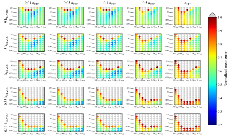
Figure 4 represents the averaged NME summed across the eight 0.09–0.9 eq. day aging exposures modeled from the BEACHON field campaign, for the NUC1 H2SO4-organics nucleation scheme and the base value of the reactive uptake coefficient, γOH, of 0.6. (A discussion of the model sensi-tivity to other values of the reactive uptake coefficient is be-low.) Figure 4 shows this average NME as a function of αEFF (effective accommodation coefficient of particles with diam-eters larger than 60 nm), kELVOC (gas-phase ELVOC frag-mentation rate constant), kOH (gas-phase functionalization rate constant), and kNUC1(rate constant for the first H2SO4 -organics nucleation scheme). Lower αEFFvalues are neces-sary for the best fits; however, there are only slight differ-ences between αEFF=0.01 and αEFF=0.05, and αEFF=0.1
(the left three columns, respectively). Faster kELVOC values are necessary for the best fits; however, similar to αEFF, the base kELVOCvalue (middle row), 3 × kELVOC, and 9 × kELVOC values show similar results, with the regions of best fits shift-ing slightly with kOH and kNUC1values. It should be noted that more gas-phase ELVOCs are being formed than could condense during the timescales of the simulated exposures (Fig. 2b). As ELVOCs would be formed more slowly in the ambient atmosphere but with a similar condensational loss timescale, nucleation is expected to proceed faster in the OFR than the ambient atmosphere. This is a reason for the potential usefulness of this OFR technique, that nucleation from chemistry of species present in ambient air can be stud-ied, even if nucleation would not be occurrent under ambient-only conditions.
For the parameter combinations of αEFF=0.01 through αEFF=0.05 and 9 × kELVOC(the top row of Fig. 4), the 2 × kNUC1 and 4 × kNUC1 values have the best fits. These 2 × kNUC1 and 4 × kNUC1 values are similar to those found by Riccobono et al. (2014) for experimental conditions at 278 K (a kNUC1value of 3.27 × 10⁻²¹cm6molec−1s−1). However, the other wells of good fits for the base kELVOC value and 3 × kELVOChave lower nucleation rate constants than that of Riccobono et al. (2014). As mentioned earlier, these kNUC1 values determined here correspond to the temperatures of the measurements (between 282 and 290 K; Table 2), which is 4– 12 K warmer than the experimental conditions of Riccobono et al. (2014); hence, we may expect lower kNUC1values due to the temperature dependence of nucleation (Yu et al., 2017). Figure 4 shows that the wells of best fits for all parameter combinations require slightly higher kOHvalues than the base kOH (based on the kOH values from Eq. 1), usually on the order of 1.5–2.5× higher.
Figures 2b and 3 show an example of the final volatil-ity distribution and size distributions for the best-fit case for an exposure of 0.23 eq. days, corresponding to the model parameters of 2 × kNUC1, 5 × kOH, 0.5 × γOH, kELVOC, and αEFF=0.01. Figure 2a and b give the initial and final parti-tionings for this case, respectively, showing that virtually all of the initial gas-phase S/IVOCs have reacted with OH to ei-ther enter the lower-volatility bins or to fragment into VOC products no longer tracked in the model. Figure 3 shows each modeled moment compared to each observed moment of the size distribution used in calculating the NME for the best-fit case.
Figures S3, S5, S7, S9, S11, S13, S15, and S17 show the same analysis as presented in Fig. 4 for each individual ex-posure modeled for the base value of γOH, 0.6. Figures S4, S6, S8, S10, S12, S14, S16, and S18 plot each observed final (OFR output) moment used in computing the NME statistic (number, diameter, surface area, and volume) compared to the six TOMAS cases with the lowest (best) NME statistic and six TOMAS cases with the highest (worst) NME statis-tic. For comparison, the observed initial (ambient air) mo-ments are also plotted for each moment.
0 200 000 dN /d lo gD p [ cm 3 ] (a) Number
Initial ambient observations Final OFR observations Best fit
Best fit with EFF=1.0
0 5000 dD p /d lo gD p [ m c m 3 ] (b) Diameter 0 250 500 dS /d lo gD p [ m 2 c m 3 ] (c) Surface area 100 101 102 Dp [nm] 0 5 dV /d lo gD p [ m 3 c m 3] (d) Volume
Figure 3. Example case of a 0.23 eq. day aging exposure from the BEACHON-RoMBAS campaign. The panels represent the moments used to calculate the normalized mean error (NME), with (a) as particle number, (b) as particle diameter (also referred to as aerosol length), (c) as particle surface area, and (d) as particle volume. The NME is calculated for each model run, using the final (OFR output) observed size distribution (black lines) compared to each model run’s final size distribution (colored lines). The solid blue lines are for the best-fit model case for this exposure, corresponding to 2 × kNUC1, 5 × kOH, 0.5 × γOH, kELVOC, and αEFF=0.01 (NME = 0.03). The dashed blue lines are for the same parameter values of the best-fit case, except that αEFF=1.0 (NME = 0.3). The vertical grey dashed lines indicate the particle size range across which the integration for calculating each mean moment was computed. The initial observed ambient size distribution (dotted black lines) is also plotted for comparison.
Figure S19 shows the same analysis as Fig. 4, but for the NUC2 nucleation scheme. It is qualitatively quite simi-lar to NUC1 but with the wells of averaged best-fit regions shifted and expanded slightly for some cases. Since we do not have measurements to further constrain the system, we acknowledge that we cannot definitively select NUC1 or NUC2 as being the better nucleation parameterization and instead note that both nucleation schemes appear to provide physically meaningful results and require further study. In contrast, Fig. 5 shows the same analyses of Fig. 4 but for the ACT nucleation scheme (Eq. 5). Figure 5 shows that there are regions of moderate NME values between 0.45 and 0.5 for αEFF=0.01 through αEFF=0.05. These regions of moderate fits occur for higher values of A (between 4 and 20 × A) for a wide range of kOH values. The best fits are seen for higher values of kELVOC(between the base value of
kELVOCand 9×kELVOC), the highest nucleation rates (for
val-ues of A between 10 and 20×A) and lower to middle rates of kOH (in general between 0.4 × kOH and the base value of kOH). In general, we do not see as good fits as we do for the NUC1 and NUC2 schemes; however, it does appear that
for some combinations of parameters, a reasonable model-to-measurement fit can be achieved with an activation nu-cleation scheme. Thus, we conclude that for this study, the H2SO4-organics mediated nucleation schemes fit the mea-surements better than the activation nucleation scheme in our model for the OFR measurements taken during the BEA-CHON campaign.
Further, as the best fits in the model come from the H2SO4 -organics mediated nucleation schemes, and the best-fit kNUC values are similar to those of Riccobono et al. (2014) where particle-phase chemistry was likely unimportant (low aerosol volume), this is indicative evidence that the creation of gas-phase ELVOCs through oxidation reactions could be dom-inant over the creation of particle-phase ELVOCs (either through accretion reactions and/or acid–base reactions) for the OFR present at the BEACHON campaign, as high con-centrations of gas-phase ELVOCs are necessary to facilitate nucleation. It is however important to note that we are lim-ited in our confidence of the actual values of the best fits of the different nucleation rate constants (kNUC1, kNUC2, and A), since each nucleation scheme is sensitive to the concentration
0.1·kOH0.4·kOHkOH 2.5·kOH10·kOH 0.05·kNUC1 0.25·kNUC1 kNUC1 4·kNUC1 20·kNUC1 9· kEL V O C 0.01· EFF 0.1·kOH0.4·kOHkOH2.5·kOH10·kOH 0.05·kNUC1 0.25·kNUC1 kNUC1 4·kNUC1 20·kNUC1 0.05· EFF 0.1·kOH0.4·kOH kOH2.5·kOH10·kOH 0.05·kNUC1 0.25·kNUC1 kNUC1 4·kNUC1 20·kNUC1 0.1· EFF 0.1·kOH0.4·kOHkOH 2.5·kOH10·kOH 0.05·kNUC1 0.25·kNUC1 kNUC1 4·kNUC1 20·kNUC1 0.5· EFF 0.1·kOH0.4·kOHkOH 2.5·kOH10·kOH 0.05·kNUC1 0.25·kNUC1 kNUC1 4·kNUC1 20·kNUC1 EFF 0.1·kOH0.4·kOHkOH 2.5·kOH10·kOH 0.05·kNUC1 0.25·kNUC1 kNUC1 4·kNUC1 20·kNUC1 3· kEL V O C 0.1·kOH0.4·kOHkOH2.5·kOH10·kOH 0.05·kNUC1 0.25·kNUC1 kNUC1 4·kNUC1 20·kNUC1 0.1·kOH0.4·kOH kOH2.5·kOH10·kOH 0.05·kNUC1 0.25·kNUC1 kNUC1 4·kNUC1 20·kNUC1 0.1·kOH0.4·kOHkOH 2.5·kOH10·kOH 0.05·kNUC1 0.25·kNUC1 kNUC1 4·kNUC1 20·kNUC1 0.1·kOH0.4·kOHkOH 2.5·kOH10·kOH 0.05·kNUC1 0.25·kNUC1 kNUC1 4·kNUC1 20·kNUC1 0.1·kOH0.4·kOHkOH 2.5·kOH10·kOH 0.05·kNUC1 0.25·kNUC1 kNUC1 4·kNUC1 20·kNUC1 kEL V O C 0.1·kOH0.4·kOHkOH2.5·kOH10·kOH 0.05·kNUC1 0.25·kNUC1 kNUC1 4·kNUC1 20·kNUC1 0.1·kOH0.4·kOH kOH2.5·kOH10·kOH 0.05·kNUC1 0.25·kNUC1 kNUC1 4·kNUC1 20·kNUC1 0.1·kOH0.4·kOHkOH 2.5·kOH10·kOH 0.05·kNUC1 0.25·kNUC1 kNUC1 4·kNUC1 20·kNUC1 0.1·kOH0.4·kOHkOH 2.5·kOH10·kOH 0.05·kNUC1 0.25·kNUC1 kNUC1 4·kNUC1 20·kNUC1 0.1·kOH0.4·kOHkOH 2.5·kOH10·kOH 0.05·kNUC1 0.25·kNUC1 kNUC1 4·kNUC1 20·kNUC1 0. 33 ·kE L V O C 0.1·kOH0.4·kOHkOH2.5·kOH10·kOH 0.05·kNUC1 0.25·kNUC1 kNUC1 4·kNUC1 20·kNUC1 0.1·kOH0.4·kOH kOH2.5·kOH10·kOH 0.05·kNUC1 0.25·kNUC1 kNUC1 4·kNUC1 20·kNUC1 0.1·kOH0.4·kOHkOH 2.5·kOH10·kOH 0.05·kNUC1 0.25·kNUC1 kNUC1 4·kNUC1 20·kNUC1 0.1·kOH0.4·kOHkOH 2.5·kOH10·kOH 0.05·kNUC1 0.25·kNUC1 kNUC1 4·kNUC1 20·kNUC1 0.1·kOH0.4·kOHkOH 2.5·kOH10·kOH 0.05·kNUC1 0.25·kNUC1 kNUC1 4·kNUC1 20·kNUC1 0. 11 ·kE L V O C 0.1·kOH0.4·kOHkOH2.5·kOH10·kOH 0.05·kNUC1 0.25·kNUC1 kNUC1 4·kNUC1 20·kNUC1 0.1·kOH0.4·kOH kOH2.5·kOH10·kOH 0.05·kNUC1 0.25·kNUC1 kNUC1 4·kNUC1 20·kNUC1 0.1·kOH0.4·kOHkOH 2.5·kOH10·kOH 0.05·kNUC1 0.25·kNUC1 kNUC1 4·kNUC1 20·kNUC1 0.1·kOH0.4·kOHkOH 2.5·kOH10·kOH 0.05·kNUC1 0.25·kNUC1 kNUC1 4·kNUC1 20·kNUC1 0.2 0.3 0.4 0.5 0.6 0.7 0.8 0.9 1.0
Normalized mean error
Figure 4. Representation of the parameter space for the average across the 0.09–0.9 day eq. aging exposures from BEACHON-RoMBAS examined in this study for the NUC1 nucleation scheme and base value of the reactive uptake coefficient of 0.6. The effective accommodation coefficient increases across each row of panels; the rate constant of gas-phase fragmentation increases up each column of panels. Within each panel, the rate constant of gas-phase reactions with OH increases along the x axis and the rate constant for nucleation increases along the y axis. The color bar indicates the normalized mean error (NME) value for each simulation, with the lowest values indicating the least error between model and measurement. Grey regions indicate regions within the parameter space whose NME value is greater than 1. No averaged case had a NME value less than 0.2 for the cases shown here.
of sulfuric acid, and in the majority of the exposures modeled we did not have a direct measurement of SO2available for all cases and instead had to estimate SO2concentrations for nearly half of the cases.
It is of note that in general, the simulations using αEFF=0.5 and αEFF=1.0 do not yield good fits for any of the nucleation schemes tested here, indicating the impor-tance of some sort of process that limits uptake to the larger aerosol. Figure 3 illustrates the impact of the effective ac-commodation coefficient for a 0.23 eq. day aging exposure: it shows each of the first four moments of the size distribu-tion for the initial and final observadistribu-tions (dotted and black lines) and for the best-fit case for this exposure (solid blue lines) and the model simulation with the same best-fit param-eter values but for αEFF=1.0 (dashed blue lines). Compared to the final observations, the best-fit case closely matches the changes in each moment for the Aitken and accumula-tion modes. However, the best-fit case with αEFF set to 1.0 clearly overestimates growth for the accumulation mode and underestimates growth for the Aitken mode. In general, when
αEFF=1.0 there was no combination of the other parameters tested that could simultaneously capture (1) the number and growth of the growing nucleation mode and (2) the change in volume of the large mode. When αEFF=1.0, either the new particles did not grow enough or the large particles grew too much throughout our parameter space. Hence, we were un-able to explain the observations without limiting the uptake of material to particles with diameters larger than 60 nm. Ad-ditionally, when we tried to lower the accommodation coeffi-cient of smaller particles (not shown), we could not simulate the growth of these particles. While our scheme for limit-ing the uptake of vapors to the large particles is very sim-ple in this study, we feel that some limitations of vapor up-take to accumulation-mode particles must be at play, possi-bly from particle-phase diffusion limitations or other reasons. Zaveri et al. (2017) modeled the controlled bimodal growth of aerosol from isoprene and α-pinene oxidation products and found that in order to replicate the observed growth, both the Aitken and accumulation modes required particle-phase diffusivity limitations. However, their experimental