Constrained optimization for hierarchical control system design

Constrained Optimization for Hierarchical

Control System Design

by

Michael Brian Jamoom, 2LT, USAF

B.S., Astronautical Engineering

United States Air Force Academy, 1997 SUBMITTED TO THE DEPARTMENT OF AERONAUTICS AND ASTRONAUTICS

IN PARTIAL FULFILLMENT OF THE REQUIREMENTS

FOR THE DEGREE OF

Master of Science

at the

Massachusetts Institute of Technology

June, 1999

©

1999 Michael B. Jamoom. All rights reserved.

The author hereby grants to MIT permission to reproduce and to distribute copies of this thesis document in whole or in part.

Signature of Autho 6

( Departmen -eronautics and Astronautics 7 May 1999 Certified by

Dr. Marc W. McConley Charles Stark Draper Laboratory Thesis Supervisor Certified by

Professor Eric Feron Assistant Professor of Aeronautics and Astronautics Thesis Advisor Accepted by

Professor Jaime Peraire Cha -- artment Graduate Committee

MAS A HUSETS INSTITUTE OF TECHNOLOGY

JUL 151999

A p

I

Constrained Optimization for Hierarchical

Control System Design

by

Michael Brian Jamoom

Submitted to the Department of Aeronautics and Astronautics on 7 May 1999 in partial fulfillment of the

requirements for the degree of Master of Science

Abstract

This thesis presents a constrained convex optimization control design procedure that takes advantage of a decoupled hierarchical system structure. To achieve a hierarchi-cal structure, a system is decoupled into primary channels that have its own dynamics, control actuator, and a resulting controller. These MIMO (multiple input/multiple output) channels are then decoupled into a hierarchical structure of SISO (single in-put/single output) loops. The constrained optimization procedure is then applied to each SISO loop to determine a solution controller.

The procedure minimizes the closed loop 712 norm as the primary objective, while presenting the Q-minimization objective as a secondary option. The procedure applies closed loop frequency and transient response constraints to the constrained optimiza-tion, which utilizes Q-parameterization of the objective function. The Q-parameter optimization decision variables are the coefficients of a stable orthogonal basis. This basis is constructed using a presented Basis Function Algorithm, designed as a con-sistent procedure for basis selection. The algorithm is designed to create the most efficient basis from three forms of basis functions: Finite Impulse Response (FIR) functions, Laguerre functions, and Legendre functions. User defined Fixed Pole Model basis functions are also addressed.

The design method is applied using the Draper Laboratory's Structural Control Toolbox (SCTB), a Computer Aided Design (CAD) tool. The design procedure is used on the Draper Small Autonomous Aerial Vehicle (DSAAV) helicopter as a design example. The solution procedure was able to make improvements in the design of the DSAAV forward motion channel. This design utilized the modularity of the hierarchical structure, using both constrained optimization and classical controller designs.

Thesis Supervisor: Dr. Marc W. McConley Title: Senior Member of the Technical Staff Thesis Advisor: Professor Eric Feron

Title: Assistant Professor of Aeronautics and Astronautics

-Acknowledgments

There are many to whom I owe a debt of gratitude for the success and completion of this thesis. I first wish to recognize those who have had direct influence on this success:

It must be understood, I cannot address any success I have in this life without first recognizing my Mom. My father died 20 years ago and my mother's strength, courage, and love focused her life to raise my brothers and myself, completely on her own. Amidst tremendous adversity, my mother ensured we had every opportunity available to succeed in life. Any success my brothers and I enjoy is a testament to her eternal dedication and support. Thank you, Mom. I love you.

I thank the Air Force, Draper Laboratory, and MIT for giving me this educational opportunity that will forever enrich my life and career. Marc McConley, my Draper thesis supervisor, I can never thank enough for his exceptional guidance and expertise that made this thesis a reality. I consider myself very fortunate to be his first master's student. He helped me when I was stuck and gave me the freedom to learn and solve my own problems. I am very grateful for Eric Feron, my MIT thesis advisor, for his diligence to continually have meetings, which motivated my continual progress with this research. His remarkable enthusiasm for research is truly inspirational.

I thank my brothers, Joe and Eric, for their support. Joe: for all those games we watched together (over the phone). Eric: for his newfound interest in sports (we're so proud of you!). I am overjoyed to recognize my sister-in-law Pam, who with Joe, delivered Matthew Daniel on February 23rd, raising the total number of confirmed living Jamooms to six.

This thesis is the monument of my 2 years in Cambridge. Those who have enhanced my life in these years are contributors to this thesis, and must be recognized.

Vik Kanwar, among my oldest friends, deserves much appreciation for his influence on my development into the person I am today. Often the first to hear my long stories, Vik taught me guitar (and some music history) and even proofread one of the last drafts of this thesis. He should sleep easy, knowing of his contribution to the military industrial complex. I also thank Marsha Pollard, who I've known just as long, for her almost daily affirmations. I'll always value our friendship, no matter how much it confuses me.

Geoff Billingsley, a fellow Air Force Draper Fellow, and I truly shared the MIT-Draper experience. Geoff, being a great friend, was a motivational workout partner, helpful class-mate, and my primary reminder of our exciting future in flight. I also recognize my Draper Fellow friends. The current Draper Fellows are Jim Smith (who will finally get rid of me), Bob Bibeau, Larry McGovern (who was always generous with his knowledge and time), Pat Brown, Chisholm Tracy, HF Vuong, and Nate Shenck, among others. Draper Fellows past include Andy Coop, Nick Nuzzo, Carla Haroz (Coach of the "Draper Monkeys"), Chris "The Man" Dever, Rudy Boehmer, Beau Lintereur, Tony Giustino, and others. I also thank Joe, the fifth floor B-core janitor, for his motivational words every evening of this semester. I must thank my roommates for enduring me on a daily basis. My first roommate, Andy, is the most stable person I know. He's a great guy that will always command my respect. Then there is Josh Kurland, my old friend and second roommate, who I thank for adding much spice (and spices) to my daily life and showing me how to get a nightlife. Josh was not only gracious enough to introduce me to his closest friends (including the wonderful Sandy and Amanda), but incorporated me into his wacky world of Harvard Law, a very amusing and rewarding experience.

I must recognize the crazy people (besides Vik and Marsha) that are my friends from home, for they remind me of my roots. Jeff Few: for road trips, Hippo in the City, and making every night a Denny's night. Kate Ogden: for the best in air mail and intense intercontinental conversations, I still wonder. Mike Brown: for bowling bets and pifiata parties. Lacey Torge: for Plymouth Rock and Sweet Kee (my private dancer). Vicki Mertz: for Atlanta layover visits (Moo!). Also thanks to Hugh Brown and Ish Beloso. I need to make a special note to Rena and the Brugmans, who are essentially an extension of the Jamoom family.

A Ta-Dow goes out to the Fellas: especially Jake Bice, who was the driving force behind all those schemes (DC, MG, the West Point body paint incident, ... ) and always brought it strong, and Todd "Treats" Smith. These Fellas constantly reminded me of the ways. Treats and AJ need to be recognized for their role in Rena's birthday surprise for me

(Thanks Rena!).

I must thank the Funny Farm for providing me with a sense of community. An enormous amount of admiration and credit goes out to Caroline Crescenzi, who had the vision to appoint me a board member. I also want to thank Funny Farmers Mary, Jody, and Chris. I also need to thank SPAMTM (for inspiration) and my Hormel Contact, Meri, for SPAMTM -Man at SPAMTM-Jam. I also need to thank Matt Fetzer and Joanna Poggione for their role in the madness.

Some extra thanks for Mona Ortman, Joy Kanwar, Doug Creviston, Cora Stubbs-Dame, Nina Erlich, Tara Harris, Mimi Martin, Aunt Frieda, The Hedins, Kristine Arrieta, Brad Head, Heather Guess, Gail Mader, Sunny Bunny, Fuzzy Eddie, Frankie Coker, the MoD, Josh's buddies: Jason, Jeremy, and Dan; Josh's Dad, Josh's friendly HLS classmates, and the T.

This thesis was prepared at The Charles Stark Draper Laboratory, Inc., under Indi-vidual Research and Development project 1012.

Publication of this thesis does not constitute approval by Draper or the sponsoring agency of the findings or conclusions contained herein. It is published for the exchange and stimulation of ideas.

Permission is hereby granted by the author to the Massachusetts Institute of Tech-nology to reproduce any or all of this thesis.

Michael B. Jamoom 7 May 1999

1 Introduction 1.1 Historical Overview ... 1.2 Contributions ... .... .... 1.3 Organization ... ... 2 Constrained Optimization 2.1 Q-Parameterization ...

2.1.1 Q Representation of the Closed Loop System . . . .

2.2

2.3

2.4

2.5

2.1.2 Q-Parameterization in State Space 2.1.3 Infinite Dimensional Representation Objective Functions ...

2.2.1 7-2 Minimization ...

2.2.2 Q-Minimization ... Basis Functions ...

2.3.1 Finite Representation of Q(z) . . . 2.3.2 Finite Impulse Response . . . . 2.3.3 Laguerre Functions ...

2.3.4 Legendre Functions ... 2.3.5 Fixed Pole Model ...

Closed Loop Constraints . . . . 2.4.1 Frequency Response Constraints . 2.4.2 Time Response Constraints . .

Model Reduction ... of Q(z) 17 17 18 19 21 23 23 24 26 26 27 28 30 30 30 31 32 32 33 33 34 35

Contents

r - - -- re

2.5.1 Balance and Truncate ... ... .. 35

2.5.2 Fractional Balanced Realization . ... 37

3 Decoupled Hierarchical System Architecture 39 3.1 System Architecture ... 40

3.2 Example of Coupled Dynamics ... 41

3.3 The Innermost Loop ... 42

3.3.1 Design of Innermost Controller and Closing the Loop .... . 43

3.4 The Intermediate Loops ... 44

3.4.1 Design of Intermediate Controller and Closing the Loop . . .. 46

3.5 The Outer Loop ... 47

3.5.1 Design of Outer Controller ... 49

4 Controller Design Solution Procedure 51 4.1 Choosing an Objective Function ... 52

4.1.1 H2 Objective Function ... 54

4.1.2 Q-Minimization Objective Function . ... 54

4.2 Setting Constraints ... 55

4.2.1 Frequency Domain Constraints . ... . . . . 55

4.2.2 Time Domain Constraints ... 56

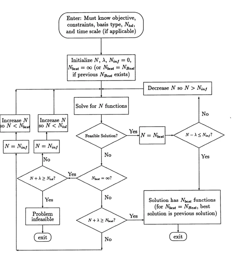
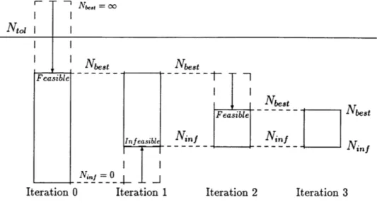
4.3 Basis Function Algorithm with Optimization Solution ... 57

4.3.1 Step 1: Best Homogeneous Basis . ... 58

4.3.2 Step 2: Best Pair Combination Basis . ... 62

4.3.3 Step 3: Best Three-Combination Basis . ... 65

4.4 Analysis and Model Reduction ... 66

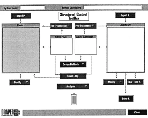
5 Structural Control Toolbox 67 5.1 Main Panel ... ... 67

5.1.1 Top Pull-Down Menus ... 68

5.1.2 Panel Menu Bars ... 69

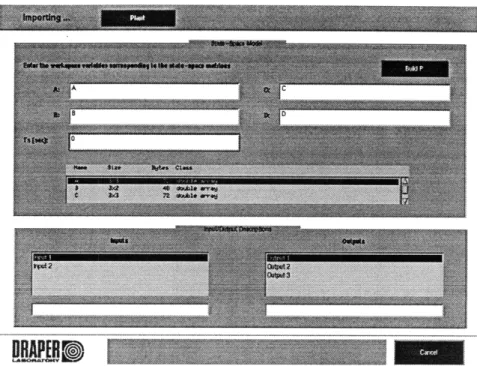
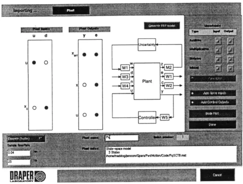
5.2 Loading a Plant Model ...

5.2.1 Defining Plant Characteristics . . . . 5.3 Constrained Optimization Controller Design . . . . 5.3.1 Setting the Objective Function . . . .

5.3.2 Editing the Basis ...

5.3.3 Editing Frequency Constraints . . . . 5.3.4 Editing Time Constraints ...

5.3.5 Solving the Optimization Problem . . . . 5.4 Analysis Tool ...

5.4.1 Analysis Options ... 5.4.2 Analysis Plots ... 5.5 Model Reduction ... 5.6 The Close Loop Tool ...

6 Draper Small Autonomous Aerial Vehicle Control 6.1 Design Objectives ...

6.2 Decoupled Hierarchical System Architecture . . . .

6.2.1 Forward Motion Dynamics . . . . 6.2.2 The Pitch Rate Loop ...

6.2.3 The Outer Three Loops . . . . 6.3 Controller Design using Solution Procedure . . . . . 6.3.1 Pitch Rate Loop: Constrained Optimization 6.3.2 6.3.3 6.3.4 6.3.5 6.3.6 6.3.7 70 . . . . . 72 . . . . . 73 . . . . . 74 . . . . 76 . . . . . 77 . . . . 78 . . . . . 80 . . . . 82 . . . . 83 . . . . 84 . . . . 85 ... 86 Example Prepa Pitch Rate Loop: Basis Function Algorithm . . . Pitch Rate Loop: Model Reduction and Analysis Solution Controllers of Outer Loops . . . . Controller Design for Coupled Forward Motion. . Q-Minimization Controller Design . . . . Observations on Constraints . . . . 89 . . . . 89 . . . . . 90 . . . . . 91 . . . . 93 . . . . . 95 S . . . . . . 95 ration . . . 96 S . . . . . . 100 S . . . . 101 S. . . . . . 104 S . . . . 107 S . . . . . . 107 S . . . . . . 108 6.4 Conclusions .. .. .. .. ... .. .. .. .. ... .. .. .. .. _ - --- ' --- -- I --108

7 Conclusions 111 7.1 Recommendations for Future Work ... 112

List of Figures

General Control Problem . . . . Q-Parameterization . . . . .

T and

Q

Depiction of System . . . . Augmented Controller Design . . . . Entire System of Coupled Channels . . . . Coupled System Architecture for a Decoupled Channel Decoupled System Architecture . . . . Generic Innermost Loop ...

Innermost Loop: Model Based Representation . . . . . Generic Intermediate Loop ...

Intermediate Loop: Model Based Representation . . . Generic Outer Loop ...

Outer Loop: Model Based Representation . . . . Flowchart of Main Solution Procedure . . . . SISO Loop with Low Pass Filter ...

Generic SISO Loop ...

Flowchart of Homogeneous Basis Reduction Procedure Basis Reduction Procedure Diagram . . . .

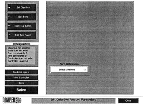
SCTB Main Panel ...

Data Input Module: MAT File Selection . . . . Data Input Module: Data Type Selection . . . . 2.1 2.2 2.3 2.4 3.1 3.2 3.3 3.4 3.5 3.6 3.7 3.8 3.9 4.1 4.2 4.3 4.4 4.5 5.1 5.2 5.3 . . . . . 40 . . . . . 41 . . . . . 42 . . . . 43 . . . . . 44 . . . . 45 . . . . . 46 . . . . 47 . . . . . 48 . . . . . 53 . . . . 54 . . . . 56 . . . . . 59 . . . . . 60 . . . . 68 . . . . . 70 . . . . . 71 .. - -- - L

5.4 5.5 5.6 5.7 5.8 5.9 5.10 5.11

5.12 Time Constraint Tool.

Constrained Optimization Control Design Panel: Analysis Tool: Initial Display . . . . Analysis Tool: Closed Loop Display Option . . LTI Viewer Output ...

Model Reduction Tool . . . . Reduction Tool ...

Closed Loop Tool ...

Closed Loop Tool: Save Panel . . . .

Post-Sol Data Input Module: State-Space Model Input Window . Data Input Module: Plant Definition Window . . . . Constrained Optimization Controller Design . . . . W72 Objective Function Control Panel . . . .

Basis Function Control Panel ...

Frequency Constraint Transfer Function Selection Panel. Frequency Constraint Tool ...

Time Constraint Transfer Function Selection Panel . . .

6.1 Entire DSAAV System of Coupled Channels . . . . 6.2 Coupled MIMO Structure for DSAAV Forward Motion . . . . 6.3 Hierarchical SISO Structure for DSAAV Forward Motion . . . . . 6.4 Pitch Rate Loop ...

6.5 Pitch Rate Loop: Model Based Representation . . . . 6.6 Pitch Rate Error Step Response: Based on Controller KqA . .. 6.7 Pitch Error Step Response: Based on Controller KOA . . ...

6.8 Forward Velocity Error Step Response: Based on Controller IKuA

6.9 Forward Position Error Step Response: Based on Controller KIxA

6.10 S(s) Frequency Constraint Based on KqA . . . . . 6.11 C(s) Frequency Constraint Based on KqA . . . . 6.12 qerr(t) Step Response Constraint . . . . .

S . . . . . . 72 S . . . . . . 73 S . . . . . . 74 S . . . . . . 75 . . . . 76 S . . . . . . 77 . . . . 78 S . . . . . . 79 . . . . 79 ution . . . . 81 . . . . . 82 . . . . . 83 5.13 5.14 5.15 5.16 5.17 5.18 5.19 5.20 97 98 99 99 100 ...

6.13 S(s) for Pitch Rate Controller Designs . ... . . . . 102

6.14 C(s) for Pitch Rate Controller Designs . ... . . . 103

6.15 Step Responses for Pitch Rate Controller Designs . ... 103

6.16 ,,rr(t) for Pitch Controller Designs . ... 105

6.17 u,,,rr(t) for Forward Velocity Controller Designs . ... 106

6.18 xer(t) for Forward Position Controller Designs . ... 106

Chapter 1

Introduction

1.1

Historical Overview

Control engineering is rooted in two main methods of solving problems: classical methods and model-based methods. Classical control methods, such as use of root-locus techniques, Bode plots, and Proportional Integral Derivative (PID) controllers infer closed-loop performance and are very effective for single input/single output

(SISO) systems. However, applying classical control to multiple input/multiple out-put (MIMO) systems is of limited value because of the coupling of the inout-puts and outputs within the dynamics. Also, classical methods deal with design specifications indirectly, requiring the control engineer to iterate by trial and error until a solution is found.

Model-based methods, such as the 7,oo and Linear Quadratic Gaussian (LQG or l1 ₂) methods, are based on state space representations of the system. These methods map the closed loop system in terms of a metric or norm. Often frequency weights are added to the input and output signals to shape the closed loop response. These weights become the design variables and are adjusted until the desired closed loop performance is achieved. Although model-based methods are effective in controlling MIMO systems, the adjustment of these design parameters is still a difficult and indirect way to design controllers.

With computer technology becoming faster and cheaper, convex optimization has

been researched as a more direct method of controller design. Convex optimization is distinct from non-convex optimization because convex optimization does not have local minima. Therefore, any minimum in a convex problem is a global minimum. Important convex optimization programs are the linear program and the quadratic program. A linear program has a linear objective, such as cTz, and linear constraints. A popular technique for solving linear programs is the Simplex Method [17]. A quadratic program has a quadratic objective function, such as x'Cz. If the constant matrix C is positive definite and the constraints are linear, then the quadratic program is convex. In the 1960s, Fegley and colleagues [2], investigated the application of linear and quadratic programming to optimal control problems.

In 1976, Youla first recognized

Q

(or Youla) parameterization [18]. In the 1980s, Q-parameterization methods of controller design were developed, applying the Q

parameter to the closed loop. Gustafson and Desoer generalized the parameterization of Q, representing

Q in terms of zero and pole locations [3, 4]. Boyd [1] and Polak [15]

used Q-parameterization in a convex optimization control design. This was done through a finite approximation of Q via basis functions. Optimization over all closed loops was reduced to an optimization over all stable Q. This is a foundation of constrained convex optimization.

Most recently, constrained optimization was successfully applied by McGovern, using 72 and £l objectives on an actual hardware system, the structural control of a telescope [9, 10]. Also, Lintereur has successfully applied constrained optimization, using the 7-2 objective, on a spacecraft attitude control system [6, 7].

1.2

Contributions

There are two main goals of this thesis. One is to uncover some benefits of decoupling a system into a hierarchical structure and applying the constrained optimization one element at a time. These benefits could range from improving optimization efficiency to taking advantage of modular control design, where controllers for separate modes (within the same channel) could be designed with completely different techniques.

The other goal is to apply constrained optimization to an actual control problem. The actual control problem presented in this thesis is the Draper Small Autonomous Aerial Vehicle (DSAAV), a helicopter.

In addition to the above goals, this thesis makes several further contributions. One such contribution is a procedure, based on constrained optimization, that solves for controllers within the hierarchical structure. Another contribution is the application of the Structural Control Toolbox (SCTB) to the solution procedure. The SCTB, developed at the Draper Laboratory, is a Computer Aided Design (CAD) toolbox which runs under MATLAB and can be very useful for many forms of controller design. This thesis explains how to apply the powerful SCTB, detailed in Chapter 5, and the benefits of this relatively new toolbox. Another useful aspect is an algorithm for choosing the most efficient basis, within the solution procedure, based on the forms of basis functions available in the SCTB. This algorithm aims at reducing the number of basis functions necessary to estimate the objective function in order to improve the speed of the optimization and produce lower order controller solutions.

1.3

Organization

The organization of this thesis falls into seven chapters. The second chapter provides developmental information for constrained optimization. This starts with a detailed explanation of how to formulate Q-parameterization into a constrained optimization problem. It then explains the different options for the portions of the constrained optimization problem: choosing an objective function, applying constraints, and se-lecting a basis function representation of Q. The chapter ends detailing the model reduction techniques necessary for applying constrained optimization to higher order systems.

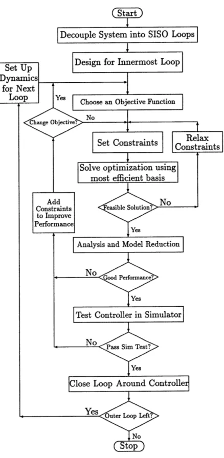
Chapter 3 details the decoupled hierarchical system architecture and how to break a coupled system into the hierarchical structure. Chapter 4 details the solution pro-cedure, complete with algorithms for choosing objective functions and setting con-straints. There is also a detailed Basis Function Algorithm in this chapter, designed

to find the most efficient basis that will provide a feasible solution. Chapter 5 ex-plains the SCTB and how to apply it to the solution procedure. Chapter 6 applies the solution procedure to the DSAAV helicopter in a control design example. Finally, the conclusions and suggestions for future work are presented in Chapter 7.

Chapter 2

Constrained Optimization

This chapter presents a brief overview of some concepts necessary for the development of the Constrained Optimization solution procedure in this thesis. It will be useful for understanding concepts and notation used in later chapters. The reader may skip this chapter if these are familiar concepts and should refer back as necessary.

A general control optimization problem is presented based on the generic system in Figure 2.1. The closed loop system H is represented by n, x n, compensator K and n, x n,, system H = .(P, K). Here, 3F(P, K) denotes the linear fractional

transformation of the plant P with the compensator K. The objective function that determines how the closed loop performance is measured is 4(H). The closed loop system H is constrained to the closed loop constraint set KH. Enough information is provided to define the following general control optimization problem.

Problem 1 Given the closed loop constraint set ICH, choose the stabilizing compen-sator K that solves the following optimization problem, minimizing the closed loop system H:

min )(H)

Kstabilizing

subject to H = Ft(P, K) E ICH

Problem 1 is a non-convex optimization problem, which is difficult to solve.

Q-parameterization (or Youla Parameterization) allows for Q-parameterization of all

_~---Figure 2.1: General Control Problem

bilizing controllers by the parameter Q. Q lies in a convex set where H is linear in

Q,

making for a convex optimization problem that is easier to solve.

This thesis will define constrained optimization as the important application of the powerful Q-parameterization allowing for convex optimization formulation. This formulation allows ICH to be mapped to convex constraints on Q. Every stabilizing compensator is related to Q through a bilinear map. The mathematical formulation is the following optimization problem [1, 7].

Problem 2 Given the closed loop constraint set ICH and the set of

Q

that closes loops

in ICH, ICQ, choose the infinite dimensional design variable Q to solve the following

optimization problem that minimizes the closed loop system H:

mmin D(H)

QEICQ

subject to ICQ = {Q stable I T, + T2QT3 E H}

H = Ti + T2QT3

The equation that defines the closed loop system H is the Q-parameterization of H, later defined as Equation 2.1.

This chapter starts, in Section 2.1, with a discussion of Q-parameterization, the parameterization technique that makes constrained optimization possible. The fol-lowing section, Section 2.2, defines the possible objective functions used to determine the performance of the optimization. Section 2.3 details basis functions and how they represent

Q.

This section explains each of the four basis functions available to create

Figure 2.2: Q-Parameterization.

the orthogonal basis for the decision variables. Section 2.4 describes how constraints on the frequency and time response are formulated into constrained optimization constraints. The final section in the chapter explains the model reduction techniques necessary for applying constrained optimization to higher order systems.

2.1

Q-Parameterization

The first step in solving the constrained optimization problem is to find the Q-Parameterization, or the Youla Parameterization [8, 18], of the closed loop system. The closed loop system is represented by n, x n, compensator K = FI(K,,

Q)

and

nz x n, system H = .TF(P, K) in Figure 2.2.

2.1.1

Q

Representation of the Closed Loop System

Q-parameterization is achieved by developing the stabilizing augmented observer-based controller Ka, with augmented control input v (added to the actuator command signal) and augmented observer error output e. The new output e becomes the input and the new input v becomes the output for the unknown stable and realizable Q

(v = Qe). For any stable

Q,

this does not change the stability of the closed loop

system. Furthermore, it is well known that the closed loop map from v to e is zero. This allows Q to appear linearly in the closed loop system H:

H = T + T2QT3 (2.1)

where T1 is the open loop map from w to z, T2 is the map from w to e, and T3 is the

map from v to z. H can now be represented by Equation 2.1 as opposed to the linear fractional representation .F(P, K). The parameterization in Equation 2.1, affine in

Q,

represents all stabilizing controllers, allowing a search over all realizable closed loop systems to be replaced by a search over all stable Q. Similar detailed discussion of Q-parameterization can be found in [1, 5, 6, 7, 8, 9, 18].

2.1.2

Q-Parameterization in State Space

The plant P maps the exogenous input w and control u to the regulated output z and measurement y as follows:

1 P2 =P [ (2.2)

y P21 P22 u u

For the compensator K, the closed loop system H is:

H = P11 + P12K(I - P222K)-'P2 1 = .T(P, K) (2.3)

For K to be internally stabilizing, H can be replaced by the Q-parameterization of Equation 2.1.

The Q parameter can be derived from any nominally stabilizing controller. The state space description of the discrete plant P is:

x[k + 1] A B1 B2 x [k]

z[k] = C Dil D12 w[k] . (2.4)

y[k] C2 D21 D22 u[k]

A controller gain matrix F and observer gain matrix G are chosen to place the eigen-values of (A - B2F) and (A - GC2) inside the unit circle to create a stabilizing

v is added to the actuator command signal. The output measurement residual e and v are described in the following equations:

v[k] = Qe[k]

u[k] = -FA[k] + v[k] (2.5)

e[k] = y[k] - Cz2i[k] - D2 2U[k]

where & represents the state estimate. A stable Q will not affect the stability of the closed loop system. After including the contribution of v to the state estimate equation, the state space representation of the augmented controller Ka is:

x[k + 1] A-B 2F-GC 2

+GD

22F G B2- GD22 &[k]

u[k] = -F 0 I y[k] (2.6)

e[k] -C 2 - D22F I -D 22 v[k]

where the space of all stabilizing controllers is spanned by K = .t(Ka,

Q)

if Q is stable.

Algebraically eliminating u and y in a lower linear fractional transformation of P and Ka results in the following state space representation of T:

x[k + 1] A + B2F -B 2F Bx B2 x[k] 0[k + 1] 0 A + GC₂ B1 + GD2 [k] (2.7)

(2.7)

z[k] C1 + D1 2F -D 1 2F Di D12 w[k] e[k] 0 C2 D21 0 v[k]

where the state estimate error & = x - x. The state estimate error is uncontrollable from v and the state x is unobservable from e. Therefore, the transfer function from

v to e is zero. Figure 2.3 shows the relationship between T and

Q.

The closed loop from w to z is:

H(z) = T1 + T2Q(I - T4Q)-1T3 = Fe(T, Q) (2.8)

where T = T1 T2 . Since T4, the transfer function from v to e, is zero,

Equa-T3 T4

tion 2.8 reduces to Equation 2.1, where the elements of T are:

T, = , , x + D12F -D12F , Dixl

0 A + GC2 B1 + GD21

(2.9)

Figure 2.3: T and Q Depiction of System

T2 = ( A + B2F, B, C, + D12F, D12 ) (2.10)

T3 = ( A+GC2, B1 + GD2 1, C2, D21 ). (2.11)

If the open loop plant is stable, the controller gain matrix F and observer gain matrix

G can go to zero. This results in T₁ = P11, T2 = P12, and T3 = P21.

2.1.3

Infinite Dimensional Representation of Q(z)

Q can be represented by an infinite number of basis functions and coefficients. This

infinite representation of Q is as follows:

00

Q(z) = : F.(z)On (2.12)

n=o

where Fn(z) is a complete set of basis functions and ,n represents the free basis function coefficients. To be complete, Fn(z) must span the space of all stable real-izable transfer functions. The relationship between this representation of Q, basis functions, and optimization, including the finite representation of Q(z), is discussed

in Section 2.3.

2.2

Objective Functions

The objective function defines how the constrained optimization measures system performance. The choice of objective function can radically alter how the problem

is formulated and the success of the resulting controller. There are various types of objective functions, and the SCTB looks at three: 7-2 minimization, Q-minimization, and l minimization. This thesis will investigate the first two: 12z minimization and Q-minimization.

2.2.1

7-2

Minimization

The most effective way to initially design a constrained optimization controller is through use of an 7-2 objective function [5]. This objective function will minimize the 7W2 norm of the transfer matrix from disturbance and noise inputs to error and control outputs. Looking back to Figure 2.2, there are two kinds of plant inputs: the exogenous input w, containing disturbances and noises, and the controller output u. Likewise there are two kinds of plant outputs: the regulated output z, containing errors and control signals, and the controller input y.

Q-Parameterization of W72 Norm

One of the most popular standards of measurement of a model-based system is the system 7-2 norm. This norm is the root mean squared (RMS) value of the system output to a given unit variance (Gaussian) white noise input. The 7W2 norm of a

MIMO system is:

1 i n, nw oo

IHl2

= Tr f H(eiw)H*(eiw)dw = E h,[k]2 _(2.13)

27r _{i=1 j=1 k=O}

where h[k] represents the closed loop impulse response.

The Q-parameterization representation of the 7-2 norm is based on the following Q-parameterization representation of the closed loop impulse response:

nu ny N-1

h1j[k] = t1,i[k] + (EE t2,ip * fnpqn * t3,qj)[k] (2.14)

p=1 q=1 n=O

where ti,ij, t2,ij, and t3,ij are the impulse responses of the (i,j) elements of T1, T2,

and T3 respectfully and the fopqn, term provides the impulse response of Q for N

finite number of basis functions f, and free coefficients qn,. I__ _

RH2 Objective Function

The 72 suboptimal objective function is the following quadratic function of pq, the vector representation of qpqn:

min Mpqpq + g p (2.15)

p=1 q=1

where the terms mjpq, gp,, and Mpq are defined as follows:

mip = t2,ip * t3,q * [fo f "... fN, (2.16)

nz n, gp = 2 / tf_{2 3} mijpq (2.17) i=1 j=1 nz nw Mpq Zm~ mT . (2.18) i=1 j=1

Once constraints are added, the 72 minimization constrained optimization problem is represented by the convex quadratic program [5]:

mm in Me + gT

subject to A0 < b

where A and b are derived from user defined constraints. Constraints are formulated in Section 2.4. Similar explanations of the 712 objective function are found in [5, 7, 9].

2.2.2 Q-Minimization

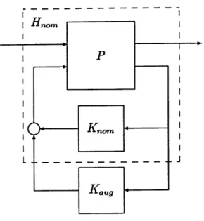
The Q-minimization technique attempts to improve upon an existing stabilizing nom-inal controller Knom. This form of constrained optimization designs an augmentation to the nominal controller. This is illustrated in Figure 2.4, where the nominal plant

P and Kom are closed to form the nominal closed loop H,,,om. The constrained

optimization design is the augmentation controller KIaug.

With the stability of the nominal closed loop system Hom as a given, an observer based Q-parameterization can occur without the observer and state feedback gains previously required to stabilize the system. This stabilizing controller KII is then combined with Q to complete the augmentation controller.

I

-I I

Figure 2.4: Augmented Controller Design

The nominal controller is then added to complete the final augmented controller K.

K = Knom + Kaug (2.20)

It cannot be stressed enough that a good K,,om is necessary. As shown in Equa-tion 2.20, any undesirable characteristics of Knom will very likely be retained in the final design.

Q-Minimization Objective Function

A good Knom is required because Q-Minimization tries to minimize the 7W2 norm of

Q,

as opposed to l12 minimization, which attempts to minimize the 7H2 norm of the

closed loop system. This way, the modifications to Knom are penalized, with the worst case scenario of Q = 0 resulting in an unaugmented Knom as the final controller. For

orthonormal basis functions, the 7?2 norm of Q is defined as follows:

nl ny N-1

IIQ(z)112

=

Z Z

qi

(2.21)

i=1 j=1 n=O

Now, the suboptimal Q-minimization objective function is:

min T¢0 (2.22)

q,

with

4

being the vector representation of Oij,. Similar explanations of the Q-minimi-zation objective function are found in [5, 7, 9].

2.3

Basis Functions

In the Q-parameterization-based optimal control formulation of Problem 2, Q repre-sented the infinite dimension design variable. As depicted in Equation 2.12, Q can be defined as a function of coefficients

4

and basis functions F(z). This can be easily approximated to a finite representation of Q with a finite number of basis functions. There are several different forms of basis functions. This thesis will focus on the four kinds of basis functions that are available in the SCTB: Finite Impulse Response (FIR), Laguerre functions, Legendre functions, and the user defined Fixed Pole Model (FPM) [5]. Further discussions on FIR and Lagaurre basis functions are found in [5, 7, 9]

2.3.1

Finite Representation of Q(z)

To make the optimization problem tractable, it is necessary to make a finite approx-imation of Q. A finite approximation of Equation 2.12 is defined below:

N-1

Q(z) . E Fn(z)¢O

(2.23)

n=O

where Fn(z) is the sequence of N stable basis functions. Now, On, the corresponding set of free coefficients, becomes the decision variables for the objective functions described in Section 2.2. It should be noted that if F(z) is orthonormal and N goes to infinity, Equation 2.23 can represent any stable transfer function.

2.3.2

Finite Impulse Response

Simplicity makes the FIR the most popular basis. The FIR formulation assumes the impulse response of Q is zero after N time steps. The FIR representation of Q(z) is:

N-1 n

Q(z) = n -. (2.24) n-30

This basis is orthonormal, satisfying the following relationship:

01 for i = i

Z

fi[k]fj[k] = for i j (2.25)

k=o 0 for i j

where the time domain form of the functions are fi[k] = S(i - k).

The FIR basis is best used for modeling fast, highly damped systems. However, if the optimal Q contains lightly damped modes or very slow dynamics, the FIR basis is less effective. Slow systems can require an inefficiently high number of basis functions

N, limiting the effectiveness of the FIR basis. It is suggested that FIR basis functions

are most effective in combination with other forms of basis functions [5].

2.3.3

Laguerre Functions

Laguerre functions are a generalization of the FIR basis. The difference between the two basis forms is Laguerre functions have their poles placed at a specified time scale

a, given that lal < 1. The FIR has all poles placed at the origin.

The discrete Laguerre basis representation of Q(z) is:

N-1 1 az -1

Q(z)

=

E

az n. (2.26)

n=O z-a z-a

Notice that for a = 0, the Laguerre basis is equivalent to the FIR basis of Equa-tion 2.24. Every transfer funcEqua-tion has an associated optimal time scale a. Similar to FIR, the Laguerre basis functions are orthonormal to each other and restrict all of the poles to one location, but the user specifies the location through the choice of a.

Selection of the Time Scale a

The number of basis functions N necessary to adequately approximate the optimal Q is directly related to the choice of a. A poorly chosen a will result in a very large basis, where a well chosen a will keep the basis size small. A well chosen a will place it close to the dominant dynamics of the optimal Q. However, selection of the best time scale and corresponding number of basis functions is hardly intuitive and often requires several design iterations. The SCTB suggests choosing a time scale with a frequency in a region where the problem is highly constrained in the frequency domain [5].

2.3.4

Legendre Functions

Legendre functions are an orthonormal set of basis functions with poles spread over a range of frequencies. This differs from the FIR and Laguerre basis, which have their functions located at the same pole. The discrete Legendre basis representation

of

Q

(z) is:

N i1 n-(1 - aiz)

Q(z) = li=O . O (2.27) n=O i=0 (z - a)

where ak = ae- (k+0.5) and lal < 1.

Selection of the Time Scale a

As with Laguerre functions, the time scales ai determine the location of the basis poles. Poles of Legendre functions are distributed across the frequency band at 0.5,

1.5, 2.5, 3.5, ... , (N - 0.5) times the frequency associated with the chosen time scale a. For example, if the chosen a has a frequency of 10 Hz, the corresponding Legendre basis would have poles located at 5 Hz, 15 Hz, 25 Hz, 35 Hz, ... , (10N - 5) Hz.

The SCTB User's Guide suggests choosing a time scale frequency no higher than the frequency of the lowest expected (non-integrator) controller pole or zero [5]. With their dynamics distributed across a range of frequencies, Legendre functions provide for a very flexible basis. This flexibility makes the Legendre functions a great initial guess for a basis.

2.3.5

Fixed Pole Model

The fixed pole model (FPM) basis allows the user to determine the pole locations of the basis. The SCTB gives the user the opportunity to define FPM poles based on the plant poles and the

Q poles, from the most recent design of

Q [5]. More information on how the SCTB allows the user to use the plant poles and Q poles can be found in Chapter 5 or [5].

2.4

Closed Loop Constraints

After defining the objective function and basis, the remaining task to complete the formulation of the constrained optimization problem is to define constraints. For the purposes of this thesis, constraints are either applied to the closed loop frequency response or the closed loop time response.

2.4.1

Frequency Response Constraints

Frequency response constraints allow the user to improve such system characteristics as command following and stability. The frequency constraints are applied as an upper bound ;iy(w) to the magnitude of a single input single output (SISO) transfer function Hij in the multiple input multiple output (MIMO) system H:

IHij(w)I 5 -y(w) (2.28)

where Hij is parameterized and discretized as follows:

nu ny N-1

Hii(z) = T1,ij +

Z Z

E T2,ipFn4,qnT3,qj. (2.29)

p=1 q=1 n=O

Breaking Hij(w) down into real and imaginary components, the constraint in Equa-tion 2.28 is equivalent to:

Re[Hij(w)] cos 0 + Im[Hij(w)] sin 0 y1ij (w) VO E [0, 27r). (2.30)

In [5, 7], this form of magnitude constraint is approximated by a finite number of linear constraints. This is done by choosing a discrete set of evenly spaced 0 between

0 and 2r:

Re[Hii(w)] cos On,N + Im[Hij(w)] sin On,N 5 7ij(w) cos N (2.31)

where n,N = - for n = 1,..., N.

After defining Sijpq(w) to be:

SijN(w) = T2,ip(w)[Fo(w) . .. FN- 1(w)]T3,qj(W) (2.32)

and defining Li(w) to be:

Lij(w) = i;j cos N - Re[T,ij(w)] cos 0,, - Im[Tl,ii(w)] sin On,N (2.33)

the approximate constraint of Equation 2.31 corresponds to a finite number of linear scalar constraints on 0:

nu ny

1 (Re[Sj,(w)] cos 9O ,N + Im[Sjpq(w)] sin0,N)Opq < Lij(w). (2.34)

p=1 q=1

With q being the vector of qpq's, Equation 2.34 is now written as Af,,req bf,,req and

can be applied to the constrained optimization problem.

2.4.2

Time Response Constraints

Constraints on time responses allow the user to try to improve output characteristics to a given input disturbance. For a closed loop MIMO system H(z), time constraints, in the form of upper bounds y,, and lower bounds 7tow, are applied to the transient response of the SISO transfer function Hij(z):

r

ow,,ij[k] 5 zij[k] 5 yup,ij[k]. 0 (2.35)

The output zij from a given disturbance wj is found by the following convolution:

zij[k] = (hij * wj)[k] (2.36)

where hij[k] is the impulse response of Hj(z). The transient response constraint of Equation 2.35 can be depicted as a constraint on 0:

nu ny

(-ow,ij - W * tl,ij)[k] E 5(wj * mijpq)[k]Opq (yup,ij - Wj * tl,ij)[k] (2.37)

p=l q=1

where mijpq is defined in Equation 2.16. With q being the vector of Opq's, Equa-tion 2.37 is now written as Atime, < btime and can be applied to the constrained optimization problem.

2.5

Model Reduction

As discussed in [1], a post optimization controller K will generally have the order of the plant plus the entire order of

Q,

which is based on the number of basis functions used to estimate Q in Section 2.3. Often, the resulting K has too high an order for implementation. If the user does not wish to implement the high order K, a form of model reduction is necessary for obtaining a reduced compensator Kred of acceptable order.

There are many forms of model reduction. For the purposes of this thesis, model reduction will be reduced to two options: Balance and Truncate and Fractional Bal-anced Reduction (FBR). The Balance and Truncate method is chosen for its widely accepted use. FBR, an extension of the Balance and Truncate method, is chosen because of its applicability to models with unstable modes.

2.5.1

Balance and Truncate

Balance and Truncate is the most widely used method for model reduction. Based on Moore's algorithm [13], Balance and Truncate relies on a Cholesky decomposition to factor the controllability and observability grammians, which then balance the system.

Balanced Realization

The first step of Balance and Truncate is to arrange the plant into an internally balanced form. A given nth order minimal stable model G(s) is defined as follows:

G(s) = C(sI - A)-1B (2.38)

where (A, B, C) is the state space representation of G(s) and I is the nth order identity matrix. The first step of balancing the plant is to solve for the observability grammian

Wo and the controllability grammian Wc in the following Lyapunov functions:

AWo + WoAT + BBT = 0 (2.39)

ATWc + WcA + CTC = 0

where Wo and We are unique, symmetric, and positive definite.

The next step is to decompose Wo with the Cholesky decomposition:

Wo = RTR. (2.41)

This is used to form the matrix RWcRT, which is subsequently diagonalized:

RWcRT = U 2_{UT (2.42)}

where UTU = I and E is defined as a diagonal matrix of Hankel singular values, ordered greatest to least (0l 2 2 ... > n):

E = diag{al,U2, ... , }. (2.43)

A Balancing Transformation Matrix 4bbal is defined as:

1

'Ibal= E-UTR. (2.44)

Now G(s) can be transformed into the minimal, internally balanced model Gbal(S):

Gbal(S) = Cbal(sI - Abal)-1'bal (2.45) where Abal = blA , Bbal = lB, and Cbal = Cj 1 . The condition for any

internally balanced plant, such as Gbal(s), is that the corresponding E is the solution to both the controllability and observability Lyapunov functions:

Abate1 + ATr + BbjBIT = AT E + EAbaj + CTCbal = 0 (2.46)

Abal E + E bT bal = Ab bal =2

Truncation of Balanced Model

The next step is to determine the size of the reduced model r, where r < n. Now the internally balanced Gbal(s) can be represented by:

[A 11 A

1

Abal = A2 Bbal B Cbal = [C1 C2] (2.47)

A2 1 A2 2 B2

where All is size r x r, B1 is size r x u (u inputs), and C1 is size y x r (y outputs).

Likewise, E is also partitioned:

E = E

(2.48)

0

E2

where El = diag{al, ₂,..., a r} and E2 = diag{ar+1, r+2,..., a,n}.

Taking the components of Equation 2.47, the truncated reduced rth order model

Gred is defined:

Gred(S) = C1(sI - A1 1)-'B 1 (2.49)

where I is the rth order identity matrix. This truncated rth order model satisfies Equation 2.46 in the following manner:

A11E1 + EIAT + B1BT = AT 1 + E1A1 1 + CTC1 = 0 (2.50)

and is, therefore, internally balanced.

Balance and Truncate only reduces stable modes of the model. Unstable modes are removed before reduction and returned to the model after reduction. Balance and Truncate can also take advantage of frequency weighting [5]. This allows the modes to be emphasized based on frequency. If a lowpass filter is used as a frequency weight, the model reduction emphasizes, and likely keeps, the low frequency states and truncates the high frequency states. Further commentary on the Balance and Truncate method can be found in [5, 11, 12, 13].

2.5.2

Fractional Balanced Realization

The Fractional Balanced Reduction method of model reduction was developed by Meyer [11, 12], extending the Balance and Truncate method. FBR allows for reduc-tion of all modes of a system, where Balance and Truncate fails to reduce unstable modes. FBR takes advantage of coprime fractional representations of the plant, gen-eralizing Balance and Truncate for all models.

FBR starts with the minimal state space representation of model G(s), as de-scribed in Equation 2.38. The first departure from Balance and Truncate is the need

---to solve the following algebraic Riccati equation (ARE):

PA + ATP - PBBTP + CTC = 0 (2.51)

where P is the positive definite solution. This step is based on a coprime fractional-ization, with the derivation found in [11, 12]. A parameter CK is defined as follows:

CK = -BTP. (2.52)

A new dynamics matrix A is defined as:

A = A + BCK. (2.53)

An entirely new state space representation is then defined as:

G(s) = C(sI - A)- 1B (2.54)

where C =

[

C . It should be noted that Equation 2.51 is now:

CK

PA + ATP + CTCK + CTC = 0 (2.55)

making P the observability grammian of this system.

FBR now returns to Balance and Truncate procedures. Using the procedure in Section 2.5.1, balance the system G(s) to get the balanced model Gbal(s). In the balanced model, Cbal = ba Then partition Gbal(s) as in Equation 2.47,

noting that C1 =

[CC1,

V

The second departure from Balance and Truncate is the partition manipulation procedure, based on coprime fractions and Graph Hankel singular vales, derived in [11, 12]. The manipulation is simplified to defining All as follows:

Al l = A1 1 - B1CK,1 (2.56)

where B1 = B1. Similar to Balance and Truncate, the rth order FBR reduced model

Gred is now:

Gred(S) = C1(SI - A1 1)-IB1 (2.57)

Chapter 3

Decoupled Hierarchical System

Architecture

This chapter presents the decoupled hierarchical system architecture, the foundation of the solution procedure found in the next chapter. Consider the example system depicted in Figure 3.1, there are four channels, one for each Cartesian position (x,y,z) and the heading 0. Each channel has an associated primary control actuator. For example, the control actuator ul is associated with the x channel. Since each channel has an associated control actuator, it is assumed each channel can have its own associated controller. For each channel, the dynamics are entirely coupled. The first decoupling separates the dynamics of the entire system into individual channels. Within each channel, more coupled dynamics exist. For the purposes of this thesis, a coupled system will be the coupled channel (which is decoupled from the other channels) as depicted in Figure 3.2. A decoupled hierarchical system will be decoupled within the channel. Here, the pertinent states are decoupled from one another as in Figure 3.3.

There are several reasons for decoupling the system into the hierarchical structure. There might be bandwidth separation between the modes of the dynamics. Decou-pling would give the control engineer the advantage of control design, one mode at a time, with the opportunity to design for each bandwidth separately. This also means that each mode can be controlled individually using multiple control techniques. The

XC r-U1 X L J y r - -I U2 LJ Dynamics

zc

r - 1 U3 z L J L__1

Figure 3.1: Entire System of Coupled Channels

hierarchical structure also simplifies the problem. Solving several decoupled SISO (single input/single output) systems is often a simpler and more computationally efficient process than solving a coupled MIMO system.

3.1

System Architecture

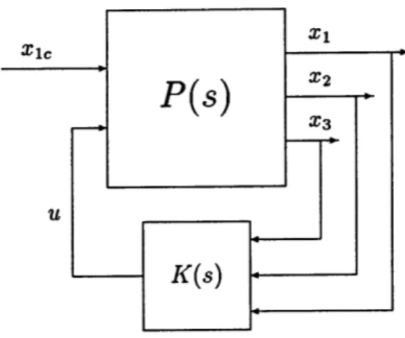
A coupled MIMO system should have a structure similar to Figure 3.2. In this structure, the input is the commanded state xlc. The commanded state is fed into

the MIMO plant P(s), where the coupled states (l,X2, 2 3) are the outputs. The outputs are fed back into the controller K(s), which then feeds the control input u into the plant. Coupling may exist between internal plant states.

For the purposes of this thesis, a decoupled system will have the hierarchical structure depicted in Figure 3.3. Here, the MIMO system is broken down into SISO inner loops. Each pertinent coupled state is allocated its own loop. The order of the loops is user defined. However, it is suggested that the state loops are ordered by having the faster and higher order derivative states in the inner loops. For example, when dealing with aircraft, tracking position and velocity profiles may be primary performance objectives. In this case, the faster attitude states (roll, pitch, yaw, and associated rates) are allocated to the more internal loops and the position states (position, velocity, and acceleration) are allocated to the outermost loops. In addition, attitude rate state loops are inside the attitude state loops and the acceleration loop

Figure 3.2: Coupled System Architecture for a Decoupled Channel comes before the velocity loop, which comes before the position loop.

The plant model is partitioned into a series of transfer functions from the control

u to the pertinent states. The error of the innermost state X3rr is the input for the

innermost loop controller K3(s), that determines the control input u. The control

input is then sent to the innermost plant P3(s), which sends out the innermost state

as an input to the next loop's plant P2(s) and as negative feedback in the innermost

loop. In the subsequent outer loops, the commanded states become the outputs of the outer controllers, with the commanded state of the outer loop xl acting as the0

original input to the system. Likewise, the outermost state xl is the last output of the system.

3.2

Example of Coupled Dynamics

The mathematical decoupling of the system starts with the state space description of the coupled dynamics P(s). For the purposes of the rest of this chapter, the example system will be the system depicted in Figure 3.2 and Figure 3.3 with three pertinent

states (x1, x2, x3) and two internal states (xi and xii). The state space representation

of the coupled system P(s) is:

i = Ax + Bu (3.1)

Figure 3.3: Decoupled System Architecture

where the dynamics matrix A and control matrix B are:

all a12 a13 ali alii bi

a2 1 a2 2 a2 3 a2i a2ii b2

A = a31 a3 2 a33 a3i a3ii B= b3 (3.2)

ail ai2 ai3 ai,i ai,ii bi

aiil aii2 aii3 aiii aii,ii bii

with the control as a sole control input u and the states are x = [Xl x2 x3 xi xi]T.

3.3

The Innermost Loop

To construct the plants of the inner loops, the dynamics that couple the pertinent states are removed and are then returned with each outer plant. For the innermost loop, the system is truncated into the innermost pertinent state and the internal states. The input to the system is the commanded innermost state.

The generic innermost loop is depicted in Figure 3.4 for R pertinent states. R = 3 for the current example, where the commanded state input is X3c. The state space representation of the innermost system G3(s), as described in Figure 3.5, has the truncated states x3 = [I₃ xi xii]T. This state space system is as follows:

3 = A3_3 + B3u_3 (3.3)

Figure 3.4: Generic Innermost Loop where

a3 3 a3i a3ii b3 0

A3 = ai3 ai,; at,it B3 = bi 0

aii3 aii,i ii,ii bi 0

(

(3.5)

-1 0 0 0 1

C3= 1 0 0 D3 = 0 0

0 0o

1 0

with the inputs u3 = [u X3c]T being the control input u and the commanded state

X3c. The outputs y = [X3err 3 u]T are the state error X3err (which is fed into the

controller), the pertinent state x3, and the control u. These are necessary outputs for

applying the solution procedure and analyzing the controller design using the SCTB in Chapter 5.

3.3.1

Design of Innermost Controller and Closing the Loop

Once the system G3(s) is defined, the innermost controller K3 is ready for design.

Fol-low the design procedure in Chapter 4 to solve for K3. The state space representation

of K3 is as follows:

-k3 = A1k 3 + Bk3X3err = -Bk 3x3 + Bk3x3c + Ak3.k 3 (3.6)

U = Ck31k₃ + Dk3X3err = -Dk3x3 + Dk3X3 + Ck3X 3 (3.7)

where k3 are the controller states of K3 and Ak3 is a nk3 X nk3 matrix. After K3 is designed, close the loop to obtain the closed loop system Ha:

.III = AIIIxIII, + B11i 3ac (3.8)

Figure 3.5: Innermost Loop: Model Based Representation

III= CIIIXIII + DIIIX3c (3.9)

where

A = A3(:, 1)- B(:, 1)Dk3 A(:, 2 : 3) Ba(:, 1)Ck3 B B3(:, 1)Dk3

-Bk3

01X2

Ak3 Bk3

1 0 0 0 0

CIII = DIII =

-Dk3 0 0 Ck3 Dk3

(3.10)

where the states are XII = [. xT3]T and the outputs are =II [x3 u]T. The

notation A3(:, 1) corresponds to the entire first column of matrix A3 and A2(:,2 : 3)

corresponds to a matrix consisting of the second through third column of matrix

A3. The input is the commanded state x3c. Once the closed loop formulation of the

innermost loop is completed, the next loop GR-1 (S) (or G2(S) for the example) can

be formulated.

3.4

The Intermediate Loops

For each intermediate loop, one pertinent state is added. This requires that state's dynamics to be returned in the formulation of the respective intermediate plant. For the intermediate loop, the system consists of the previous inner pertinent states and the internal states. The input to the system is the commanded intermediate state.