HAL Id: hal-02873023
https://hal.inria.fr/hal-02873023
Submitted on 18 Jun 2020
HAL is a multi-disciplinary open access
archive for the deposit and dissemination of sci-entific research documents, whether they are pub-lished or not. The documents may come from teaching and research institutions in France or abroad, or from public or private research centers.
L’archive ouverte pluridisciplinaire HAL, est destinée au dépôt et à la diffusion de documents scientifiques de niveau recherche, publiés ou non, émanant des établissements d’enseignement et de recherche français ou étrangers, des laboratoires publics ou privés.
Three-dimensional physics-based registration of pelvic
system using 2D dynamic magnetic resonance imaging
slices
Hadrien Courtecuisse, Zhifan Jiang, Olivier Mayeur, Jean-Francois Witz,
Pauline Lecomte-Grosbras, Michel Cosson, Mathias Brieu, Stéphane Cotin
To cite this version:
Hadrien Courtecuisse, Zhifan Jiang, Olivier Mayeur, Jean-Francois Witz, Pauline Lecomte-Grosbras, et al.. Three-dimensional physics-based registration of pelvic system using 2D dynamic magnetic resonance imaging slices. Strain, Wiley-Blackwell, 2020, 56 (3), �10.1111/str.12339�. �hal-02873023�
DOI: xxx/xxxx
FULL PAPER
3D Physics-based Registration of Pelvic System Using 2D Dynamic
MRI Slices
H. Courtecuisse
1,2| Z. Jiang
3| O. Mayeur
4,5| J.-F. Witz
4,5| P. Lecomte
4,5| M. Cosson
6,7| M.
Brieu
4,5| S. Cotin
21AVR/ICube Strasbourg, France, France 2Inria, Nancy, France
3Univ. Lille, UMR 9189 - CRIStAL - Centre de Recherche en Informatique Signal et Automatique de Lille, France
4Centrale Lille, Villeneuve d’Ascq, France 5CNRS, Lille, France
6CHU Lille, Service de Chirurgie Gynécologique, France
7Univ. Lille, Faculté de Médecine,France
Correspondence
*H. Courtecuisse, Email: [email protected]
This paper introduces a method for dynamic 3D registration of female pelvic organs using 2D dynamic magnetic-resonance images (MRI). The aim is to provide a better knowledge and understanding of pathologies such as prolapsus or abnormal mobility of tissues. 2D dynamic MRI sequences are commonly used in nowadays clinical routines in order to evaluate the dynamic of organs, but due to the limited view, subjectivity related to human perception cannot be avoided in the diagnoses. A novel method for 2D/3D registration is proposed combining 3D Finite Element models with a priori knowledge of boundary conditions, in order to provide a 3D extrapolation of the dynamic of the organs observed in a single 2D MRI slice. The method is applied to the 4 main structures of the female pelvic floor (bladder, vagina, uterus and rectum), providing a full 3D visualization of the organs’ displacements. The methodology is evaluated with two patient-specific data sets of volunteers presenting no pelvic pathology, and a sensitivity study is performed using synthetic data. The resulting simulations provide an estimation of the dynamic 3D shape of the organs facilitating diagnosis compared to 2D sequences. Moreover, the method follows a protocol compatible with current clinical constraints presenting this way potential short term medical applications.
KEYWORDS:
2D-3D Registration; Pelvic system simulation; Constraint-Based Simulation; Augmented Reality
1
INTRODUCTION
Female genital prolapse is mainly characterized by excessive mobility of organs resulting from the weakness of the pelvic floor. It is a common pathology related to the age of women: over 60 years old, more than 60% of women suffer from it, while the average percentage is from 20% to 30% for women of all ages combined [33, 34]. According to the severity of the symptoms, surgery may be necessary. Magnetic Resonance Imaging (MRI) is often chosen for the evaluation of female pelvic pathology because this technique provides high contrast resolution without any radiation [13]. Dynamic MRI images
are widely used in nowadays clinical routines [30] to capture the dynamic of organs’ motion while the patient is breathing or pushing. However, the requirements of high image resolu-tion limit the current dynamic MRI protocols to 2D slices with a frequency of acquisition between 2 and 4 images per second. Due to the limited field of view, subjectivity related to human perception as well as medical experience cannot be avoided and causes variability in the diagnoses.
Moreover, some anatomical suspension structures (ex. fas-ciae and ligaments) are hardly observable in MRI, but play a key role in organs’ mobility [25]. As stated by recent publica-tions [10, 25], the development of a mobility analysis tool is a major challenge to better understand the complex behavior
of organs, which is still not fully understood today, in order to provide relevant medical diagnosis and adapted surgery to cure the patient.
The contribution of this work is an automatic image-based tracking method providing the outline of organs in a set of 2D dynamic MRI images acquired during the diagnosis, that is later combined with 3D biomechanical models in order to extrapolate the complete 3D dynamic motion of structures. The ill-posed nature of the 2D/3D registration problem is reduced adding a priori knowledge of boundary conditions in order to constrain off-plane motions around the image’s plane. Although the location and the mechanical properties of boundary conditions are generally not know accurately, the patient-specific data extracted from the segmentation of images are combined with generic models of suspension struc-tures generated semi automatically thanks to previous works [25]. Contrary to pure image-based methods which generally provide information limited to images’ plane, the proposed approach allows to significantly reduce the 3D displacement error, even where no data are available, allowing this way to estimate the complete kinematics of the pelvic system during the dynamic sequence.
Finally, a strong consideration was given to follow the limi-tations of current clinical routines in order to provide potential short term clinical applications. The resulting 3D analysis of motion allows for better identification of potential pathology.
2
RELATED WORKS
During the last decade, patient-specific models of the pelvic system have been developed thanks to advances in experimen-tal tests on soft tissues, mathematical modeling and computer simulations [25]. To evaluate pelvic organs’ mobility Finite Element (FE) simulations have been used [37, 20], providing better understanding of the mechanisms involved in physiolog-ical or pathologphysiolog-ical cases [7, 24]. Organs’ mobility is linked to mechanical properties of soft tissues, material modeling and anatomical suspension structures of the pelvic system. Indeed, [36] shows the necessity to take into account the suspension system, which is located out of the dynamic MRI plane and is rarely observed on static MRI. To improve the bio-fidelity of FE model Lecomte et al. [21] proposed a method for geomet-rical reconstruction based on medical imaging using dynamic MRI and digital image correlation, combined with anatomical knowledge and analysis of the measured displacement fields. However, the validity domain of the models remains limited to small deformations which prevent the method for the simula-tion of pathology such as prolapses involving large abnormal mobility of tissues.
As aforementioned, concerning the problems related to pelvic floor disorders, biomechanical FE models have also been involved for a proper personalized cure for patholog-ical conditions, especially the POP (pelvic organ prolapse). Generally, applying a FE simulation requires principally the following elements : medical images providing observations and ground truth data, geometries of pelvic organs and struc-tures, characterization of mechanical properties and definition of boundary conditions. Promising results have been made on each of these aspects. In [38], the study focused on the mechanical properties of vaginal tissue of women. The stiff-ness was evaluated by using a scanning haptic microscope. A comparison of tissue of women with and without POP was carried out and the relation with collagen composition was shown. [36, 37] provided useful preliminaries to the simula-tions of pelvic cavity behaviors. FE simulasimula-tions were applied to a multi-organ model of a patient, focusing on the ligamentous boundary conditions definition. As in [12, 23, 26], more recent works proposed a solution of the three-dimensional FE mod-eling of the pelvic floor towards the patient-specific modmod-eling. [26] demonstrated 3D FE simulation of the pelvic cavity under larger strain. Less complex pelvic organ models were involved in these works [12, 23], but a special attention has been paid to the patient-specific aspect and to the clinical application. Based on anatomical and surgical expertise, some important structures were turned into parameters that can be specifically defined, including the presence of muscles, hiatus size, vagi-nal dimension, fascia length, etc. Results were reported with respect to pelvic organ prolapse quantification system (POP-Q). In parallel with the previous contributions, [3, 16, 15] dealt with the issue of geometric modeling of pelvic organs that had not been treated in these contributions. [3] presented a method to reconstruct hollow organs with a thickness from pre-segmented points cloud. In [16], a more efficient approach was proposed to generate readily usable CAD (Computer Assisted Design) pelvic geometries for FE simulations. The geome-try construction was validated by using a controlled physical model [15]. The idea is to reduce the gap in the processing pipeline from MRI to FE simulations.
Real-time registration of biomechanical models have also been used for intra-operative 3D registration with 2D dynamic MRI. In [9, 35], a model of a pig’s liver is registered with 2D slices during breathing motion. Although the authors have shown that the method allows for the estimation of off-plane motions, it is limited to a single organ and requires the syn-chronization of 3 orthogonal slices which is not possible in a realistic clinical scenario. The methods cited above perform the registration prescribing displacements which significantly reduces the importance of both mechanical parameters and
boundary conditions of biomechanical models in the neighbor-hood of image’s data [27]. Yet, in areas where no data are avail-able models plays the role of a regularization term between image-based constraints [32]. In this case, the mechanical parameters as well as boundary conditions can be at least as important as the constitutive law itself [4]. Mechanical studies and rheological experiments can provide generic infor-mation about the mechanical action of boundary conditions [25]. Peterlik et al. [31] showed that the mechanical action of boundary conditions can be directly extracted from the biomechanical registration process.
This paper introduces a method for the registration of 3D FE models with material points located on the contours of organs in dynamic 2D MRI images. Compared to the previous works, this work pays more attention to the pelvic motions, using dynamic MRI as one of the ground truth data. An extensive survey can be found in [11] for 2D slices to 3D volume reg-istration problems. A constrained-based optimization problem is solved using image features, biomechanical models, and anatomical connection. The originality of the proposed solu-tion lies in the fact that the FE simulasolu-tion is driven by image data in the plane coordinate of the 2D dynamic slices, while FE models provide an estimation of off-plane motions. The ill-posed nature of the problem is compensated by adding a priori knowledge of boundary conditions (ligaments, contacts between structures...) during the registration, providing this way a mechanical extrapolation of dynamic MRI data. Results show that adding a priori knowledge of the mechanical action of the tissues (ligaments, contacts...) allows to significantly reduce off-plane errors and provide additional information than what is observed in 2D images.
3
EXPERIMENTAL PROTOCOL
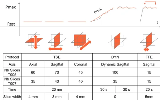
In this section the experimental protocol allowing for acquisi-tion of the necessary data for the simulaacquisi-tion and the evaluaacquisi-tion of the method is detailed. Patient-specific data are generated from two data sets of two volunteers (designed as T005 and T007 in the rest of the paper), presenting no pelvic pathology. The experimental data inputs have been acquired following a close protocol to a standard clinical routine (see Figure 1 ).
3.1
Dada acquisition
Pelvic MRI requires between 20 to 50 minutes to obtain static volume images of organs (TSE) with sufficient resolution. The procedure is then immediately followed by a dynamic acqui-sition (DYN) while the patient is contracting and relaxing the pelvic muscles. DYN sequence is performed following the middle plane, the most representative of the organs’ motion.
Data have been obtained with a 3-Tesla MR (Philips Achieva 3.0T TX) providing up to 2 images per second in a dynamic mode. Although this frequency is sufficient to capture the dynamic of tissues, the whole volume movement is not visible and its evaluation relies on the physician’s experience.
TSE and DYN are already parts of standard clinical routines, but a final step (FFE) is added in order to evaluate the accuracy of the registration method. The volunteers are asked to main-tain a maximal contraction of pelvic muscles without moving nor breathing. This significantly limits the time allowed for the acquisition. 15 sparse sagittal slices uniformly distributed in the volume have been acquired. Although FFE is not necessary to perform the registration, it provides the only available data to evaluate the accuracy of the method.
3.2
Data and mesh generation
The pelvic floor is a complex system where multiple organs act together during the deformation. In this paper 4 organs are con-sidered (Vagina, Uterus, Bladder and Rectum), whose geome-tries are obtained from the segmentation of TSE images (see Figure 2 ). Vagina and rectum are injected with gel to enhance image contrast and facilitate the segmentation procedure.
In addition to the geometries of organs, anatomical support-ing structures are added in order to constrain the mobility of organs and thus provide a more realistic cinematic. The car-dinal and uterosacral ligaments represent the structures main-taining the cervix and the uterus which are modeled as attached constraints to link the vagina and uterus. Paravaginal ligaments located on both sides of the vagina are also modeled to sustain the model in position and fixed at their extremities. Finally, fas-ciae between pelvis and bladder and the one between rectum and sacrum are taken into account. The ligaments and fas-ciae are not visible in the clinical images. Their geometries are obtained from anatomic literature and an iterative optimization process described in [25].
4
TRACKING IN DYNAMIC MR IMAGES
The visible outline corresponding to each organ in the DYN MR sequence will be used to impose displacements during the simulation (Section 5.1). Nevertheless, the semi-automatic tracking of organs’ outline in DYN MR images is difficult because it requires to find tangential information that can-not be obtained directly by using the image contrast. Recent works introduced a method for multiple organs detection in MR images based on B-spline model [18]. This method is used to fit an initial B-spline model for each organ at the beginning of the sequence (see Fig 3 ).
Pmax
Rest t
Protocol TSE DYN FFE
Axis Axial Sagittal Coronal Dynamic Sagittal Sagittal
Nb Slices T005 60 70 45 100 15 Nb Slices T007 35 40 40 35 15 Time 20 mn 30 s 30 s 20 s Slice width 4 mm 3 mm 4 mm 0 5mm
FIGURE 1 Protocol for MRI data acquisition composed of three steps. TSE: Volume acquisition is performed providing the
geometry of organs. DYN: a dynamic 2D sequence is acquired during breathing and contraction of muscles. FFE: A sparse volume acquisition is performed for the validation, while the volunteer maintains a maximal pressure of organs.
(a) Segmentation
(b) FE models
FIGURE 2 Initial segmentation and meshing. (left) the
seg-mentation is performed using TSE images. (right) FE models are generated from the segmentation and boundary condition are added to complete the FE model.
For each image, it is important to follow material points of the contour over time with maximum precautions, especially to avoid drifting along the contour boundaries. Additional feature-sensitive constraints are added in order to better track the material points and to ensure the plausibility of the com-puted motion [17]. These constraints consist in the detection of corner points of high curvature in order to impose normal movements of the tracked points. Based on the initial B-spline model [18], each organ is then redefined by a composite Bézier curve (a series of segments attached end to end). The begin-ning and ending points of Bézier segments are considered as material points, selected automatically based on the criteria of
high curvature. As shown in Figure 3 , [𝐩𝐟0,𝐩𝐟1,⋯ , 𝐩𝐟𝑙] are
the selected points. Then, the contour is deformed to fit the other images in the DYN sequence, by minimizing iteratively an energy term (more details can be found in [17]).
Figure 4 shows the semi-automatic tracking of four high-lighted organs with material points: bladder (red), vagina (blue), rectum (green) and uterus (light blue). Given the poor contrast of the uterus in the image, its contour is roughly gener-ated using optical flow. For each image 𝑖, the 2𝐷 points of the contour are reconstructed in 3𝐷 according to the slice
coordi-nates, providing a set of points 𝐦(𝑖)located on the surface of
each organ. With respect to the mobility of different areas, the distribution of points matches the organs shape.
During the dynamic sequence, the set of points 𝐦(𝑖) may
not necessarily be associated with the same material points on the 3𝐷 surface of the models. Indeed, being located in a
unique 2𝐷 plane position, 𝐦(𝑖) may represent the outline of
several cross section of the organ (in case of translations or rotations of the tissues in the orthogonal direction of the image slice). Therefore, sliding constraints are introduced in order to prescribe displacements of biomechanical models in the plane while minimizing the mechanical energy of numerical models and to estimate the entire 3𝐷 displacements.
p0=pf0 p3=pf1
p1
p2
Curvature Selected features [pf0, pf1, ... pfl] Composite Bezier curve
FIGURE 3 The tracking principle: an organ contour defined by a composite Bezier curve, the joined points (features) are
selected by high curvatures. For each segment, from images 𝑡 to 𝑡 + 1, the transformation of features is computed by Optical
Flow [22, 5] and the adjustment of free control points (𝐩1, 𝐩2) is perpendicular to the segment. Such process is repeated until
the end of the sequence.
FIGURE 4 Outline tracking with material points in the
sequence of dynamic MR images.
5
CONSTRAINT-BASED REGISTRATION
OF BIOMECHANICAL MODELS
FE models are meshed using linear tetrahedral elements1, and
internal forces are computed following a corotational formu-lation [29]. The co-rotational model was mainly used in the field of computer graphics [28], but this formulation is more and more used for medical simulations due to its low com-putational cost. The corotational approach is used in order to enforce the stability of the simulation and maintain computa-tion time compatible with clinical constraints, while allowing for the simulation of large deformations.
The corotational model is parametrized with the Poisson ratio 𝜈 and the young modulus 𝐸 chosen for an average model in the literature (see [24] and [10] for details). The discrete for-mulation of elastic forces applied on the nodes of a tetrahedral element 𝑒 can be written as:
𝒇𝑒= 𝐑𝑒𝐊𝑒(𝐑 𝑇
𝑒𝐪̄𝑒− 𝐪𝑒) (1)
where ̄𝐪𝑒and ̄𝐪𝑒are respectively the initial and deformed
posi-tions of the nodes of the hexahedron and 𝒇𝑒, the elastic forces
1Note that the method is not dependent on the type of element nor the con-stitutive law. For instance, surface FE models such as Thin-Shell models and hyper-elasticity could be used as employed in [25].
applied on these nodes. While 𝐊𝑒 corresponds to the local
linear stiffness matrix of the element, parametrized by the
Young’s modulus E and the Poisson’s ratio 𝜈, 𝐑𝑒is a block
diagonal matrix defined as:
𝐑𝑒= ⎛ ⎜ ⎜ ⎜ ⎜ ⎝ 𝐑 𝟎 𝐑 𝐑 𝟎 𝐑 ⎞ ⎟ ⎟ ⎟ ⎟ ⎠ (2)
with 𝐑 being the 3 × 3 rotation matrix of the tetrahedral element. The rotation matrices of each element are evalu-ated independently using a polar decomposition of the strain displacement, allowing this way for higher ranges of deforma-tions.
The local stiffness matrix 𝐊𝑒 can be written with the
syn-thetic formulation:
𝐊𝑒= 𝐑𝑒 ∫ 𝑉𝑒
(𝐂𝑒𝐃𝑒𝐂𝑒𝜕𝑉𝑒)𝐑𝑇𝑒 (3)
where 𝐂𝑒 and 𝐃𝑒 are respectively the strain-displacement
matrix and the stress-strain matrix. While these matrices are
constant during the simulation, 𝐑𝑒needs to be updated at each
iteration providing this way a geometrically nonlinear constitu-tive model allowing the simulation of large displacements but small deformations.
5.1
Constraints definition
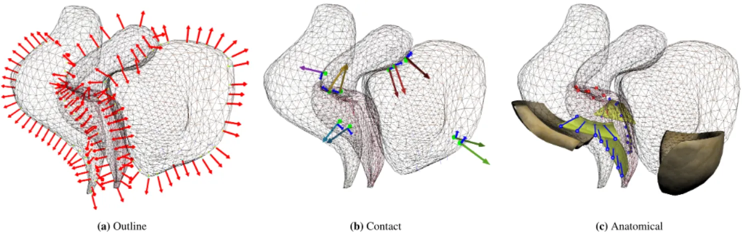
During the simulation 3 types of constraints are used to deform the models (see Figure 5 ):
Sliding Constraint 𝜔: Due to off-plan motions, control points 𝐦 cannot be associated with constant coordinates on organs’ surfaces. Therefore, to impose constraints, an Iterative Closest Point (ICP) method is used: at the beginning of each
(a) Outline (b) Contact (c) Anatomical
FIGURE 5 Constraints set used in the simulation: Outline constraints (left), Contact Constraints (center), Anatomical
constraints (right).
simulation step, control points are associated with their respec-tive nearest triangle on the surface of the segmented models. In addition, the ICP method is modified to enforce that the normal of the surface aim in the same direction as the normal of the contour computed in the image. Formally, Sliding Constraints are described by the following equation:
𝜔(𝐧𝑠,𝐪𝑠,𝐦) = 0 (4)
where 𝐦 are the tracked points in the 2D image and 𝐪𝑠their
respective closest point on the surface of FE models. 𝐧𝑠are the
associated normal of points 𝐪𝑠that are projected in the image
plane in order to impose displacements in the 2D image’s space and fit the outline in DYN MRI, while enforcing no orthogonal forces in 3D. This formulation allows the FE models to slide in the orthogonal direction and reduce the energy of the system to perform the registration (see [9] for details).
Contact Constraints 𝜙: Taking into account contacts is fundamental to avoid unnatural configurations such as the interpenetration of organs outside of DYN plane. Contacts pro-vide additional constraints that prevents unrealistic rotations of organs around the constraint DYN plane. When point con-tacts exist in the system, the concon-tacts form separation distance constraints:
𝜙(𝐪𝑐)≥ 0 (5)
which means that positions in contact 𝐪𝑐 of FE models must
remains on the positive side of the surface normals. A volume-based method relying on the computation of Layered Depth Images (LDI) (see [1] for details) is used to perform the col-lision detection between structures. Volume-based methods are robust to deep intersections, which are unavoidable due to data noise and approximations in the reconstruction process. Friction is also added to prevent large lateral motion between organs due to the presence of connective tissues.
Anatomical Constraints 𝜒 : Anatomical constraints are added to limit the off-plane motion of organs (see Figure 5 c). The vagina is attached at each side by ligaments reconstructed semi-automatically using the method introduced in [25] and meshed with regular hexahedral elements. Bilateral constraints are added between the vagina and ligaments allowing the ver-tical mobility but penalizing lateral motions. The uterus is attached to the vagina with bilateral constraints (red), linking the displacement of both structures. These constraints can be formalized with:
𝜒(𝐪𝑣,𝐪𝑢) = 0 (6)
where 𝐪𝑣 and 𝐪𝑢are the attached positions of the vagina and
uterus. In addition, fasciae constrain lateral motions of the bladder and the rectum on each side. Since these structures are not visible in the images, their precise location and geome-tries are not known and may change during the sequence. In order to avoid the generation of unsolvable problems where the outline of the organs overlaps the initial geometries of faciae during the dynamic motion, these structures are considered deformable with fixed constraints on their extremity. Faciae are attached to the rectum and the bladder with bilateral constraints remaining this way in contact with tissues while deformations allow satisfying images constraints.
While 𝜔 are derived from visible images’ data and used to drive models, other constraints are instead added as a-priori knowledge of organs’ behavior to prevent unrealistic behaviors (such as interpenetration) and reduce the number of solutions of the ill-posed 2𝐷∕3𝐷 registration problem.
5.2
Solving Process
For each DYN MR image (every 0.25 sec in average), a static problem is solved to find equilibrium between internal
elastic forces and constraint forces applied to satisfy image data. Nevertheless, a dynamic formulation is chosen to inte-grate the simulation models over time. Indeed, even if the motion is prescribed within the MRI plane (where dynamic is already provided by images), off plane displacements are entirely driven by the models where dynamic is necessary. In addition, dynamic integration allows stabilizing the problem and in the absence of external forces, it incrementally iterates toward a static equilibrium solution.
FE’s governing equation is given by the following dynamic equations:
𝐌 ̈𝐪+(𝐪) + (𝐪, 𝐦(𝑖))𝝀 = 𝟎 (7)
where (𝐪) are internal volume forces (given by the
co-rotational formulation, which corresponds to equation (1).) depending on positions 𝐪 and velocities ̇𝐪 of FE models. 𝐌 is the mass matrix used to integrate the dynamic of the sys-tem and numerically stabilize the syssys-tem. The mass of organs
are parametrized according to the literature2.(𝐪, 𝐦(𝑖)) is a
non-linear function gathering the set of constraints applied on the models 𝜔, 𝜙 and 𝜒 . This function takes as input 𝐪 and
𝐦(𝑖)which are, respectively, the position of the FE models and
the set of points extracted from an image 𝑖 and reconstructed in 3D. Its formulation is linearized at each simulation step (see below). Lagrange multipliers 𝝀 are used to impose the constraints.
For each simulation step, the nodal velocities ̇𝐪 and nodal positions 𝐪 are updated following a backward Euler Implicit method. The nodal accelerations ̈𝐪 at the end of the time step 𝑡
are given by ̇𝐪𝑡+ℎ= ̇𝐪𝑡+ ℎ ̈𝐪𝑡+ℎand 𝐪𝑡+ℎ= 𝐪𝑡+ ℎ ̇𝐪𝑡+ℎ, where
ℎ is the simulation time step. Yet, since several images are
acquired per second in the DYN sequence, very small dis-placements are observed between images, and dynamic effects in the image plane remains limited. ℎ is mainly used as a parameter to control the number of iterations of the iterative solver described below, and it does not influence the converged configurations of the models.
Since ̇𝐪𝑡+ℎ and 𝐪𝑡+ℎ are unknown, the non-linear problem
defined in equation (7) is linearized (equivalent to a first order Taylor expansion). Assuming that no constraints 𝝀 are applied
at the beginning of each simulation step 𝑡 (i.e. 𝝀𝑡 = 𝟎, see [27]
for details) it gives: [ 1 ℎ𝐌+ ℎ 𝜕 𝜕𝐪||||𝐪 𝑡 ] (𝐪𝑡+ℎ− 𝐪𝑡) = −(𝐪𝑡) (8)
In addition, constraint equations, are linearized at the begin-ning of each simulation step and assumed constant during the
2note that mass parameters do not have any influence at equilibrium state since no gravity is applied
time step. It can be written as follows:
𝐇𝑇(𝐪𝑡+ℎ−𝐪𝑡) = 𝜹, with 𝐇 = [ 𝜕𝜔 𝜕𝐪 ||||𝐪𝑡 ; 𝜕𝜙 𝜕𝐪 || || |𝐪𝑡 ; 𝜕𝜒 𝜕𝐪 || || |𝐪𝑡 ] (9) where 𝐇 is known as the Jacobian of the constraints. This matrix includes both the direction in which the contact forces
𝝀 are applied and the Degrees of Freedom of the models
impacted by the constraints to cancel the penetration 𝜹. These directions are obtained either from the ICP method (for 𝜔 constraints) or from the collision detection (for contact con-straints).
The combination of the non-linear constraint equations, provides a KKT (Karush-Kuhn-Tucker) problem:
{
𝐀𝐱+ 𝐇𝝀 = 𝐛
𝐇𝑇𝐱 = 𝜹 (10)
where 𝝀, 𝐱 = (𝐪𝑡+ℎ− 𝐪𝑡) and 𝜹 are unknown; 𝐛 = −(𝐪𝑡) and
𝐀= 1 ℎ𝐌+ ℎ
𝜕
𝜕𝐪||||𝐪
𝑡
(see [8] for details).
The Schür complement method is used to solve the aug-mented linear system, involving the computation of the
com-pliance matrix 𝐖 = 𝐇𝐀−1𝐇𝑇 that relates the mechanical coupling between constraints. This matrix is computed in real-time with GPU parallelization as details in [8].
The constraint problem is solved with an iterative Gauss-Seidel algorithm which allows for fast definition of non-linear contact forces (such as friction). More importantly the iter-ative solver provides stable solutions even in case of non-convergence of the solver. Indeed, since most of our constraints depend either on image data or specific simulated positions (for the ICP); it is difficult to guarantee the well-posedness of the constraint problems. This may result in redundant or even antagonist constraints which prevent the use of direct solvers.
6
RESULTS
Based on patient-specific data, the evaluation of the method is limited to the fact there are no imaging modalities allow-ing retrievallow-ing the complete 3D displacements of organs durallow-ing the registration process. Therefore, after introducing the mesh generation procedure, a synthetic evaluation of the method is described providing quantitative results of the dynamic 3D motion. Then the method is applied to the patient specific data described above. The 15 FFE Sagittal images have been segmented manually providing a coarse representation of the organs’ geometries at maximal pressure state (see Figure 8 a). The evaluation of the method is compared to the ground truth at the final state of the dynamic acquisition using manually segmented positions in the FFE slices.
6.1
Mesh generation
Real-time FE models have been generated and integrated in
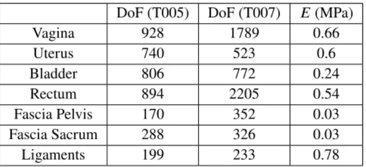
Sofa3(see table 1 ). Since the considered organs are
membra-nous structures, hollow tetrahedral FE models were generated from an extrusion of a constant thickness of their surface allowing this way for compression with high resistance in elon-gation, except for the uterus which is discretized with a full volume of tetrahedral elements. In addition, the ligaments and fascia, are not visible in the clinical images. Specific FE models have been generated semi-automatically (see [24]) and meshed with regular grids of hexahedral elements. These supporting structures are considered fixed at their extremities, far from the interactions with the other organs.
DoF (T005) DoF (T007) 𝐸(MPa)
Vagina 928 1789 0.66 Uterus 740 523 0.6 Bladder 806 772 0.24 Rectum 894 2205 0.54 Fascia Pelvis 170 352 0.03 Fascia Sacrum 288 326 0.03 Ligaments 199 233 0.78
TABLE 1 Number of degrees of freedom (DoF) and Young’s
modulus (𝐸) of the FE models used for the registration. The characterization of pelvic tissues has been extensively studied [2]. Yet, mechanical parameters in patient specific sce-narios are subject to variability. Therefore, all the following simulations have been run 100 times, where the mechanical parameters of each model have been randomized within a range of 10% around the values given in the table 1 . The following results include the average error and the standard deviation of this simulations set.
6.2
Synthetic evaluation
A numerical FE simulations have been performed on Abaqus software using the data of the patient T005. The convergence of the FE simulation, as well as a mesh sensitivity, was car-ried out in order to guarantee the validity of the results. The hyperelastic behavior of the soft tissues of the pelvic system is taken into account thanks to previous published works [6]. We assume that the material is homogeneous. Based on the semi-automatic detection on MRI [16], a FE model is gener-ated thanks to shell elements for the organs (vagina, bladder, rectum) and pelvic floor [26]. Ligaments are also considered with truss elements to mimic the sustainable structures, as they
3https://www.sofa-framework.org
play a key role in the organ’s mobility [12]. The average dis-placement of the vagina was 8.2 mm in the dynamic image plane. Although the displacement is small compared to med-ical data, this simulation provides the complete 3D motion of structures allowing this way to obtain quantitative evaluations of the accuracy of the registration during the dynamic process. Nodal displacements of meshes in the Abaqus simulation have been exported for 15 simulation steps, allowing this way to generate both the ground truth and similar input data as described in the experimental protocol of the section 3. Each position is then successively played during 3 simulation steps in Sofa while performing the registration. For this purpose, the outline of organs was generated from the intersection of Abaqus’ models and the image plane coordinates of the 2D dynamic MRI sequence. These positions are used to impose displacements of meshes in Sofa.
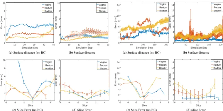
Figure 6 (top) reports the average distance between posi-tions extracted in Abaqus (uniformly sampled every 5 mm over the complete surface of organs) and the closest surface trian-gle of the registered models for the complete process; while taking into account or not (left/right) the boundary conditions. Even if models are only driven by a set of constraints located in a single plane, the registration procedure allows maintain-ing an average error smaller than 4 mm over the entire 3D volume for any deformation step. In addition, the error of the vagina is reduced by a factor 2 when taking into account the suspension structures and boundary conditions, allowing this way for the complete 3D extrapolation of off-plane motion. In addition, Figure 6 (bottom) shows the average error at the final state (step 45) measured as the intersection of organs’
sur-faces with the 15 FFE slices acquired in the medical data4. As
expected, the error is minimal at the location where constraints are imposed (index 0). However, the error remains small for all the other slices located both sides side of the constraint slice (positive and negative indexes). In addition, although the method provides similar accuracy results in the dynamic plane, error increases significantly faster when boundary con-ditions are not taken into account. This is because the off-plane motion results in non-realistic rotations of organs around the constrained plane.
The numerical simulation in Abaqus relies on small per-turbations theory and only focuses on the movement at the beginning of motion to ensure numerical stability. In order to evaluate the accuracy of method with larger motion, FE models have been registered with the set of tracked positions obtained in the dynamic MRI slice (see section 4). The accuracy of the registration with respect to medical data will be detailed in the next section. Instead, the generated motion is first used
4Note that the 3D geometry of organs does not necessarily cross all the val-idation slices and does not necessarily have values for all the columns in the graphs.
10 20 30 40 50 0 2 4 6 8 10 Simulation Step Error (mm) Vagina Rectum Bladder
(a) Surface distance (no BC)
10 20 30 40 50 0 2 4 6 8 10 Simulation Step Error (mm) Vagina Rectum Bladder (b) Surface distance -6 -4 -2 0 2 4 0 2 4 6 8 10 Slice Error (mm) Vagina Rectum Bladder
(c) Slice Error (no BC)
-6 -4 -2 0 2 4 0 2 4 6 8 10 Slice Error (mm) Vagina Rectum Bladder (d) Slice Error
FIGURE 6 Evaluation of the registration method using the
simulation generated with Abaqus.
50 100 150 200 0 2 4 6 8 10 12 14 Simulation Step Error (mm) Vagina Rectum Bladder
(a) Surface distance (no BC)
50 100 150 200 0 2 4 6 8 10 12 14 Simulation Step Error (mm) Vagina Rectum Bladder (b) Surface distance -6 -4 -2 0 2 4 6 0 2 4 6 8 10 12 14 Slice Error (mm) Vagina Rectum Bladder
(c) Slice Error (no BC)
-6 -4 -2 0 2 4 6 0 2 4 6 8 10 12 14 Slice Error (mm) Vagina Rectum Bladder (d) Slice Error
FIGURE 7 Evaluation of the registration method using the
simulation generated with Sofa. to perform a sensitivity study of the method with respect to
mechanical parameters.
During the dynamic sequence, the maximal displacement of the vagina was measured above 2.5 cm. Figure 7 reports the errors of the proposed solution with this data set. As previ-ously, the method allows maintaining a small distance between the simulated surfaces and the registered shapes. However, in this scenario the importance of anatomical constraints is enhanced since it allows to reduce the average error by a factor 4× for the vagina and 2× for the other organs. More importantly, when boundary conditions are not simulated, the standard deviation related to the uncertainty of mechanical parameters is almost null because image-based constraints 𝜔 does not depend on the mechanical parameters but only on the geometry of the models. Therefore, the resulting deforma-tions always converge to similar situadeforma-tions, providing higher errors, without taking into account the mechanical behavior of structures. When adding the boundary conditions, the method still provides reproducible results (small standard deviation) independently of the chosen parameters within the range of variability. Finally, similar conclusions are obtained at the final step when the errors are measured independently for each val-idation slice (FFE), i.e. the error increase significantly faster with respect to the distance of the constraint plane, when boundary conditions are not taken into account.
6.3
Patient-specific application
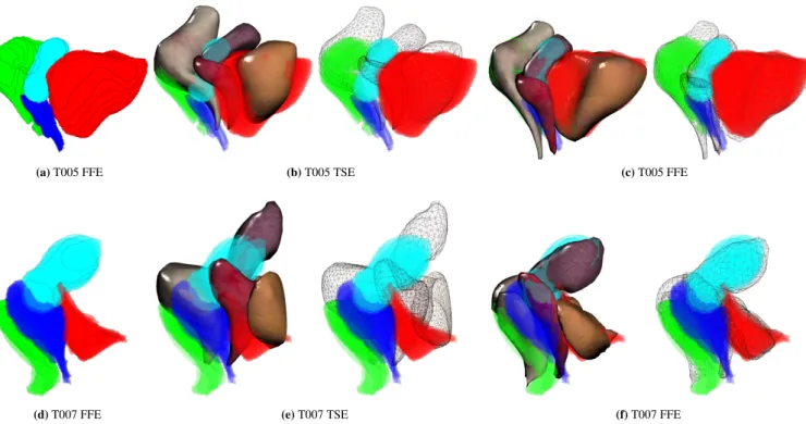
The method has been applied with the two patient-specific data of the volunteers. An overlapping with the organs’ geome-tries at the final state is shown in Figure 8 . Results show that complex motion and deformations happened, enhancing the need for biomechanical models during the registration: For T005 the vagina has been significantly displaced and con-tracted, leading to the compression of the rectum and sliding of the uterus along the bladder. For T007, the bladder is com-pressed by surrounding tissues and the fasciae which result in a significant modification of the geometry of the organ. Our method provides realistic transitions including far from the image plane.
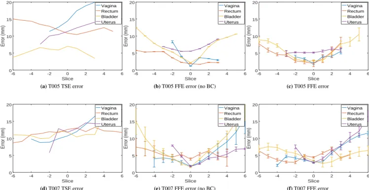
The average distance error according to FFE segmentation is reported in Figure 9 . Results show that our biomechanical registration allows to significantly reduce the error in the 2D DYN plane (index 0) where constraints are applied, but it can also provide an accurate extrapolation for off-plane motion. The vagina undergoes the most important displacement where an average error between TSE and FFE surfaces are initially around 15𝑚𝑛 and reduced to 3𝑚𝑚 using our method. A pos-sible explanation of the remaining error can be related to the significant amount of contrast gel expelled during the dynamic acquisition (due to compression of muscles) which is not taken into account in current FE models. As observed with synthetic data, boundary conditions allow not only to decrease the off-plane errors far from the image constraint, but they also prevent
(a) T005 FFE (b) T005 TSE (c) T005 FFE
(d) T007 FFE (e) T007 TSE (f) T007 FFE
FIGURE 8 Overlapping between sparse FFE segmentation (8 a) and organs’ geometries for both before (8 b) and after (8 c)
the dynamic registration.
the simulated models to produce unrealistic and non-physically possible configurations such as rotations of organs around the constrained plane or inter-penetrations.
Finally, despite the complex interactions and the high num-ber of degrees of freedom, all the above simulations achieved a fixed frame rate of 14 frames per second with data T005 and 8 FPS with T007 on an Intel(R) Core(TM) i9-9900K CPU @ 3.60GHz and a GeForce RTX 2070. Each simulation step involves on average 30 non-linear friction contact constraints with 70 outline constraints. Given the acquisition time of the MRI, the frame rate it is sufficient to perform real-time simu-lation of the MRI sequence (i.e. 1 second can be simulated in 1 second). Therefore, apart from the segmentation and meshing of TSE images, this method open the possibility of real-time diagnosis and planning of the future surgery. Indeed, the real-time computation offer the possibility to evaluate the influence of mechanical structures and the effect of boundary conditions for future planning assistance of the surgery.
7
CONCLUSION AND DISCUSSION
A method for semi-automatic registration of pelvic organs has been proposed which is compatible with nowadays clini-cal routines. The method relies on the registration of 3D FE models to 2D dynamic MRI slices, providing a biomechan-ical extrapolation for off-plane dynamic motion of organs.
The method has been validated with patient specific data of two volunteers. This approach allows moving towards the patient-specific treatment. Indeed, this work based on medi-cal imaging and numerimedi-cal simulation would make it possible to better understand pelvic mobility and to study the poten-tial defects related to the equilibrium of pelvic statics [19]. The care can be adapted more precisely to the pathology in a specific way using a numerical FE model. The method leads to interesting results linking medical imaging process to the definition of the pelvic organs mobility and the stress-strain equilibrium. Understanding the impact of surgical techniques to treat the patient is essential for the development of more
effective surgical prolapse repair [14]. Numerical
simula-tions of the organ’s mobility allow to advance our knowledge on the impact of various surgical techniques and to improve surgical decision-making on the choice of techniques, by con-sidering the mobility of organs with this method. Moreover, preoperative simulation could enable the results of a surgical procedure to be predicted and the technique to be adapted to the individual patient.
Acknowledgement: This work was supported by French National Research Agency
(ANR) within the project SPERRY ANR-18-CE33-0007.
References
[1] Allard, J., F. Faure, H. Courtecuisse, F. Falipou, C. Duriez, and P. Kry, 2010: Volume Contact Constraints at Arbitrary Resolution. ACM Transactions on
-6 -4 -2 0 2 4 6 0 5 10 15 20 Slice Error (mm) Vagina Rectum Bladder Uterus
(a) T005 TSE error
-6 -4 -2 0 2 4 6 0 5 10 15 20 Slice Error (mm) Vagina Rectum Bladder Uterus
(b) T005 FFE error (no BC)
-6 -4 -2 0 2 4 6 0 5 10 15 20 Slice Error (mm) Vagina Rectum Bladder Uterus (c) T005 FFE error -6 -4 -2 0 2 4 6 0 5 10 15 20 Slice Error (mm) Vagina Rectum Bladder Uterus (d) T007 TSE error -6 -4 -2 0 2 4 6 0 5 10 15 20 Slice Error (mm) Vagina Rectum Bladder Uterus
(e) T007 FFE error (no BC)
-6 -4 -2 0 2 4 6 0 5 10 15 20 Slice Error (mm) Vagina Rectum Bladder Uterus (f) T007 FFE error
FIGURE 9 Average distance error (mm) according to the index of FFE Sagittal planes. Index 0 corresponds to the location of
DYN slices (i.e. where constraints are applied).
Graphics, 29, no. 3.
[2] Baah-Dwomoh, A., J. McGuire, T. Tan, and R. De Vita, 2016: Mechani-cal Properties of Female Reproductive Organs and Supporting Connective Tissues: A Review of the Current State of Knowledge. Applied Mechanics
Reviews, 68, no. 6, 060801.
[3] Bay, T., J.-C. Chambelland, R. Raffin, M. Daniel, and M.-E. Bellemare, 2011: Geometric modeling of pelvic organs. Conference proceedings : ... Annual International Conference of the IEEE Engineering in Medicine and Biology Society. IEEE Engineering in Medicine and Biology Society. Annual Confer-ence, 2011, 4329–4332, doi:10.1109/IEMBS.2011.6091074.
URL http://www.ncbi.nlm.nih.gov/pubmed/22255297
[4] Bosman, J., N. Haouchine, J. Dequidt, I. Peterlik, S. Cotin, and C. Duriez, 2014: The Role of Ligaments: Patient-Specific or Scenario-Specific ?
Inter-national Symposium on Biomedical Simulation ISBMS, Strasbourg, France.
[5] Brox, T. and J. Malik, 2011: Large displacement optical flow: descriptor matching in variational motion estimation. IEEE Transactions on Pattern
Analysis and Machine Intelligence, 33, no. 3, 500–513.
[6] Chantereau, P., M. Brieu, M. Kammal, J. Farthmann, B. Gabriel, and M. Cos-son, 2014: Mechanical properties of pelvic soft tissue of young women and impact of aging. International Urogynecology Journal, 25, no. 11, 1547– 1553.
[7] Chen, L., J. A. Ashton-Miller, and J. O. L. DeLancey, 2009: A 3d finite element model of anterior vaginal wall support to evaluate mechanisms underlying cystocele formation. Int. J. Biomech., 42, no. 10, 1371–1377. [8] Courtecuisse, H., J. Allard, P. Kerfriden, S. P. A. Bordas, S. Cotin, and
C. Duriez, 2014: Real-time simulation of contact and cutting of heterogeneous soft-tissues. Medical Image Analysis, 18, no. 2, 394–410.
[9] Courtecuisse, H., I. Peterlík, R. Trivisonne, C. Duriez, and S. Cotin, 2014: Constraint-Based Simulation for Non-Rigid Real-Time Registration. MMVR. [10] Egorov, V., H. Van Raalte, and V. Lucente, 2012: Quantifying vaginal tissue elasticity under normal and prolapse conditions by tactile imaging.
Inter-national Urogynecology Journal and Pelvic Floor Dysfunction, 23, no. 4,
459–466.
[11] Ferrante, E. and N. Paragios, 2017: Slice-to-volume medical image registra-tion: A survey. Medical Image Analysis, 39, 101 – 123.
[12] Gordon, M. T., J. O. L. DeLancey, A. Renfroe, A. Battles, and L. Chen, 2019: Development of anatomically based customizable three-dimensional finite-element model of pelvic floor support system: Pop-sim1.0. Interface Focus,
9, no. 4, 20190022.
[13] Hamm, B. and R. Forstner, Eds., 2007: Diagnostic Imaging - MRI and CT of
the Female Pelvis. Diagnostic Imaging, Springer-Verlag Berlin Heidelberg.
[14] Jeanditgautier, E., O. Mayeur, M. Brieu, G. Lamblin, C. Rubod, and M. Cos-son, 2016: Mobility and stress analysis of different surgical simulations during a sacral colpopexy, using a finite element model of the pelvic system.
International Urogynecology Journal, 27, no. 6, 951–957.
[15] Jiang, Z., O. Mayeur, L. Patrouix, D. Cirette, J.-F. Witz, J. Dumont, and M. Brieu, 2020: Patient-specific modeling of pelvic system from mri for numerical simulation: Validation using a physical model. Computational
Biomechanics for Medicine, M. P. Nash, P. M. Nielsen, A. Wittek, K. Miller,
and G. R. Joldes, Eds., Springer International Publishing, Cham, 19–30. [16] Jiang, Z., O. Mayeur, J.-F. Witz, P. Lecomte-Grosbras, J. Dequidt, M. Cosson,
C. Duriez, and M. Brieu, 2019: Virtual image correlation of magnetic reso-nance images for 3d geometric modelling of pelvic organs. Strain, 55, no. 3, e12305, doi:10.1111/str.12305.
[17] Jiang, Z., J.-F. Witz, P. Lecomte-Grosbras, J. Dequidt, S. Cotin, C. Rubod, C. Duriez, and M. Brieu, 2017: Multiorgan motion tracking in dynamic mag-netic resonance imaging for evaluation of pelvic system mobility and shear strain. Strain, 53, no. 2, e12224.
[18] Jiang, Z., J. F. Witz, P. Lecomte-Grosbras, J. Dequidt, C. Duriez, M. Cos-son, S. Cotin, and M. Brieu, 2015: B-spline based multi-organ detection in magnetic resonance imaging. Strain, 51, no. 3, 235–247.
[19] Lamblin, G., O. Mayeur, G. Giraudet, E. JeanditGautier, G. Chene, M. Brieu, C. Rubod, and M. Cosson, 2016: Pathophysiological aspects of cystocele with a 3d finite elements model. Archives of Gynecology and Obstetrics, 294, no. 5, 983–989.
[20] Lecomte-Grosbras, P., M. Nassirou - Diallo, J.-F. Witz, D. Marchal, J. Dequidt, S. Cotin, M. Cosson, C. Duriez, and M. Brieu, 2013: Towards a better understanding of pelvic system disorders using numerical simulation. Medical Image Computing and Computer Assisted Intervention - MICCAI.
Nagoya, Japan, 16, no. Pt 3, 307–314.
[21] Lecomte-Grosbras, P., J.-F. Witz, M. Brieu, N. Faye, M. Cosson, and C. Rubod, 2015: Quantification of pelvic mobility on dynamic magnetic reso-nance images: Using mechanical insight to help diagnose pelvic pathologies.
Strain., 51, no. 4, 301–310.
[22] Lucas, B. D. and T. Kanade, 1981: An iterative image registration technique with an application to stereo vision. IJCAI, volume 81, 674–679.
[23] Luo, J., L. Chen, D. E. Fenner, J. A. Ashton-Miller, and J. O. L. DeLancey, 2015: A multi-compartment 3-d finite element model of rectocele and its interaction with cystocele. Journal of Biomechanics, 48, no. 9, 1580 – 1586. [24] Mayeur, O., G. Lamblin, P. Lecomte-Grosbras, M. Brieu, C. Rubod, and M. Cosson, 2014: FE Simulation for the Understanding of the Median Cysto-cele Prolapse Occurrence. Biomedical Simulation, 220–227.
[25] Mayeur, O., J. F. Witz, P. Lecomte-Grosbras, M. Brieu, M. Cosson, and K. Miller, 2016: Influence of Geometry and Mechanical Properties on the Accuracy of Patient-Specific Simulation of Women Pelvic Floor. Annals of
Biomedical Engineering, 44, no. 1, 202–212.
[26] Mayeur, O., J.-F. Witz, P. Lecomte-Grosbras, M. Cosson, and M. Brieu, 2019: Patient-specific simulation: Non-destructive identification method for soft tissue under large strain: Application to pelvic system. Computational
Biomechanics for Medicine, P. M. F. Nielsen, A. Wittek, K. Miller, B. Doyle,
G. R. Joldes, and M. P. Nash, Eds., Springer International Publishing, Cham, 131–144.
[27] Morin, F., H. Courtecuisse, I. Reinertsen, F. Le Lann, O. Palombi, Y. Payan, and M. Chabanas, 2017: Brain-shift compensation using intraoperative ultra-sound and constraint-based biomechanical simulation. Medical Image Analy-sis, 40, 133–153, doi:10.1016/j.media.2017.06.003.
[28] Müller, M., J. Dorsey, L. McMillan, R. Jagnow, and B. Cutler, 2002: Stable real-time deformations. Proceedings of the 2002 ACM
SIGGRAPH/Euro-graphics symposium on Computer animation - SCA ’02, ACM Press, New
York, New York, USA, 49.
[29] Müller, M. and M. Gross, 2004: Interactive virtual materials. GI ’04: Proc.
of Graphics Interface 2004, School of Computer Science, University of
Waterloo, Waterloo, Ontario,Canada, 239–246.
[30] Pannu, H. K., H. S. Kaufman, G. W. Cundiff, R. Genadry, D. A. Bluemke, and E. K. Fishman, 2000: Dynamic MR imaging of pelvic organ prolapse: Spectrum of abnormalities 1. Radiographics, 20, no. 6, 1567–1582. [31] Peterlik, I., H. Courtecuisse, C. Duriez, and S. Cotin, 2014: Model-Based
Identification of Anatomical Boundary Conditions in Living Tissues.
Infor-mation Processing in Computer Assisted Interventions, Fukuoka, Japan.
[32] Peterlik, I., H. Courtecuisse, R. Rohling, P. Abolmaesumi, C. Nguan, S. Cotin, and S. E. Salcudean, 2017: Fast Elastic Registration of Soft Tissues under Large Deformations. Medical Image Analysis.
[33] Samuelsson, E. C., F. T. Arne Victor, G. Tibblin, and K. F. Svärdsudd, 2015: Signs of genital prolapse in a Swedish population of women 20 to 59 years of age and possible related factors. American Journal of Obstetrics &
Gynecology, 180, no. 2, 299–305.
[34] Swift, S. E., 2015: The distribution of pelvic organ support in a population of female subjects seen for routine gynecologic health care. American Journal
of Obstetrics & Gynecology, 183, no. 2, 277–285.
[35] Trivisonne, R., I. Peterlik, S. Cotin, and H. Courtecuisse, 2016: 3D Physics-Based Registration of 2D Dynamic MRI Data. MMVR - Medicine Meets
Virtual Reality, Los Angeles, United States.
[36] Vallet, A., C. Rubod, J.-F. Witz, M. Brieu, and M. Cosson, 2011: Simulation of pelvic mobility: topology optimisation of ligamentous system. CMBBE, 14, no. sup1, 161–162.
[37] Venugopala Rao, G., C. Rubod, M. Brieu, N. Bhatnagar, and M. Cosson, 2010: Experiments and finite element modelling for the study of prolapse in the pelvic floor system. Computer methods in biomechanics and biomedical
engineering, 13, no. 3, 349–357.
[38] Zhou, L., J. Lee, Y. Wen, C. Constantinou, M. Yoshinobu, S. Omata, and B. Chen, 2012: Biomechanical properties and associated collagen compo-sition in vaginal tissue of women with pelvic organ prolapse. Journal of