HAL Id: hal-00403913
https://hal.archives-ouvertes.fr/hal-00403913
Submitted on 13 Jul 2009HAL is a multi-disciplinary open access archive for the deposit and dissemination of sci-entific research documents, whether they are pub-lished or not. The documents may come from teaching and research institutions in France or abroad, or from public or private research centers.
L’archive ouverte pluridisciplinaire HAL, est destinée au dépôt et à la diffusion de documents scientifiques de niveau recherche, publiés ou non, émanant des établissements d’enseignement et de recherche français ou étrangers, des laboratoires publics ou privés.
Alessandro Morbidelli, William Bottke, David Nesvorny, Harold Levison
To cite this version:
Alessandro Morbidelli, William Bottke, David Nesvorny, Harold Levison. Asteroids Were Born Big. Icarus, Elsevier, 2009, in press. �hal-00403913�
Alessandro Morbidelli Observatoire de la Cˆote d’Azur
Boulevard de l’Observatoire B.P. 4229, 06304 Nice Cedex 4, France
William F. Bottke Southwest Research Institute
1050 Walnut St, Suite 300 Boulder, CO 80302 USA
David Nesvorn´y Southwest Research Institute
1050 Walnut St, Suite 300 Boulder, CO 80302 USA
Harold F. Levison Southwest Research Institute
1050 Walnut St, Suite 300 Boulder, CO 80302 USA
ABSTRACT
How big were the first planetesimals? We attempt to answer this question by conducting coagulation simulations in which the planetesimals grow by mutual collisions and form larger bodies and planetary embryos. The size frequency dis-tribution (SFD) of the initial planetesimals is considered a free parameter in these simulations, and we search for the one that produces at the end objects with a SFD that is consistent with asteroid belt constraints. We find that, if the initial planetesimals were small (e.g. km-sized), the final SFD fails to fulfill these con-straints. In particular, reproducing the bump observed at diameter D ∼ 100 km in the current SFD of the asteroids requires that the minimal size of the ini-tial planetesimals was also ∼100km. This supports the idea that planetesimals formed big, namely that the size of solids in the proto-planetary disk “jumped” from sub-meter scale to multi-kilometer scale, without passing through interme-diate values. Moreover, we find evidence that the initial planetesimals had to have sizes ranging from 100 to several 100 km, probably even 1,000 km, and that their SFD had to have a slope over this interval that was similar to the one characterizing the current asteroids in the same size-range. This result sets a new constraint on planetesimal formation models and opens new perspectives for the investigation of the collisional evolution in the asteroid and Kuiper belts as well as of the accretion of the cores of the giant planets.
1. Introduction
The classical model for planet formation involves 3 steps. In Step 1, planetesimals form. Dust sediments towards the mid-plane of the proto-planetary disk and starts to collide with
each other at low velocities. The particles eventually stick together through electrostatic forces, forming larger fractal aggregates (Dominik and Tielens, 1997; Kempf et al., 1999; Wurm and Blum, 1998, 2000; Colwell and Taylor, 1999; Blum et al., 2000). Further collisions make these aggregates more compact, forming pebbles and larger objects. A bottleneck for this growth mode is the so-called meter-size barrier. The origin of this barrier is two-fold. On the one hand, the radial drift of solid particles towards the Sun due to gas drag reaches maximum speed for objects roughly one meter in diameter. These meter-size boulders should fall onto the Sun from 1 AU in 100 to 1,000 years (Weidenschilling, 1977), i.e. faster than they can grow to significantly larger sizes. On the other hand, because gas drag is size dependent, bodies of different sizes spiral inwards at different velocities. This leads to mutual collisions, with relative velocities typically several tens of meters per second for bodies in the centimeter- to meter-size range. Moreover, in turbulent disks, even equal-size bodies collide with non-zero velocities due to turbulent stirring. This effect is again maximized for meter-size boulders (Cuzzi and Weidenschilling, 2006; see also Dominik et al., 2007). Current theories predict the destruction of the meter-sized objects at these predicted speeds (Wurm et al., 2005). In the absence of a well understood mechanism to overcome the meter-size barrier, it is usually assumed that Nature somehow manages to produce planetesimals of 1 to 10 km in diameter, objects that are less susceptible to gas-drag and all of its hazardous effects.
In Step 2, planetary embryos/cores form1. Collisional coagulation among the
1 The embryos are objects with Lunar to Martian masses, precursor of the terrestrial
planets, that are expected to form in the terrestrial planets region or in the asteroid belt. In the Jovian planet region, according to the core-accretion model (Pollack et al., 1995), the giant planet cores are multi-Earth-mass objects that eventually lead to the birth of the giant planets by gas accretion.
planetesimals allows the latter to agglomerate into massive bodies. In this step gravity starts to play a fundamental role, bending the trajectories of the colliding objects; this fact effectively increases the collisional cross-section of the bodies by the so-called
gravitational focussing factor (Greenzweig and Lissauer, 1992). At the beginning, if the
disk is dynamically very cold (i.e. the orbits have tiny eccentricities and inclinations), the dispersion velocity of the planetesimals vrel may be smaller than the escape velocity of the
planetesimals themselves. In this case, a process of runaway growth begins, in which the relative mass growth of each object is an increasing function of its own mass M, namely:
1 M dM dt ∼ M1/3 vrel ,
(Greenberg et al., 1978; Wetherill and Stewart, 1989). However, as growth proceeds, the disk is dynamically heated by the scattering action of the largest bodies. When vrel becomes
of the order of the escape velocity from the most massive objects, the runaway growth phase ends and the accretion proceeds in an oligarchic growth mode, in which the relative mass growth of the largest objects is proportional to M−1/3
(Ida and Makino, 1993; Kokubo and Ida, 1998). The combination of runaway and oligarchic growth produces in the inner Solar System a population of planetary embryos, with Lunar to Martian masses (Wetherill and Stewart, 1993; Weidenschilling et al., 1997). In the outer Solar System, beyond the so-called snowline (Podolak and Zucker, 2004), it is generally expected that the end result is the formation of a few super-Earth cores (Thommes et al., 2003; Goldreich et al., 2004; Chambers, 2006) that, by accretion of a massive gaseous atmosphere from the disk, become giant planets (Pollack et al., 1996; Ida and Lin, 2004a,b; Alibert et al., 2004, 2005).
In Step 3 the terrestrial planets form. The system of embryos in the inner Solar System becomes unstable and the embryos start to collide with each other, forming the terrestrial planets on a timescale of several 107 to ∼ 108 years (Chambers and Wetherill, 1998; Agnor
Kenyon and Bromley, 2006). Of all the steps of planet formation, this is probably the one that is understood the best, whereas Step 1 is the one that, because of the meter-size barrier, is understood the least.
How can the meter-sized barrier be overcome? Two intriguing possibilities come from a recent conceptual breakthrough; new models (Johansen et al., 2007; Cuzzi et al., 2008) show that large planetesimals can form directly from the concentration of small solid particles in the turbulent structures of the gaseous component of the protoplanetary disk. Here we briefly review the models of Johansen et al. (2007) and Cuzzi et al. (2008).
Johansen et al. (2007) showed that turbulence in the disk, either generated by the Kelvin-Helmoltz instability (Weidenschilling, 1980; Johansen et al., 2006) or by Magneto-Rotational Instability (MRI; Stone et al., 2000), may help the solid particles population to develop gravitational instabilities. Recall that turbulence generates density fluctuations in the gas disk and that gas drag pushes solid particles towards the maxima of the gas density distribution. Like waves in a rough sea, these density maxima come and go at many different locations. Thus, the concentration of solid particles in their vicinity cannot continue for very long. The numerical simulations of Johansen et al. (2006, 2007), however, show that these density maxima are sufficiently long-lived (thanks also to the inertia/feedback of the solid particles residing within the gas, the so-called streaming instability; Youdin and Goodman, 2005) to concentrate a large quantity of meter-size objects (Note that the effect is maximized for ∼ 50 cm objects, but we speak of meter-size boulders for simplicity). Consequently, the local density of solids can become large enough to allow the formation of a massive planetesimal by gravitational instability. In fact, the simulations in Johansen et al. (2007) show the formation of a planetesimal with 3.5 times the mass of Ceres is possible within a few local orbital periods.
that chondrule size particles are concentrated and size-sorted in the low-vorticity regions of the disk. In fact, Cuzzi et al. (2008) showed that in some sporadic cases the chondrule concentrations can become large enough to form self-gravitating clumps. These clumps cannot become gravitationally unstable because chondrule-sized particles are too strongly coupled to the gas. Consequently, a sudden contraction of a chondrule clump would cause the gas to compress, a process which is inhibited by its internal pressure. In principle, however, these clumps might survive in the gas disk long enough to undergo a gradual contraction, eventually forming cohesive planetesimals roughly 10-100km in radius, assuming unit density. This scenario has some advantages over the previous one, namely that it can explain why chondrules are the basic building blocks of chondritic planetesimals and why chondrules appear to be size-sorted in meteorites. Interestingly, Alexander et al. (2008) found evidence that chondrules must form in very dense regions that would become self-gravitating if they persist with low relative velocity dispersion.
The models described in Johansen et al. (2007) and Cuzzi et al. (2008) should be considered preliminary and semi-quantitative. There are a number of open issues in each of these scenarios that are the subject of on-going work by both teams. Moreover, there is no explicit prediction of the size distribution of the planetesimals produced by these mechanisms or the associated timescales needed to make a size distribution. Both are needed, if we are to compare the results of these models with constraints. Nevertheless, these scenarios break the paradigm that planetesimals had to be small at the end of Step 1; in fact, they show that large planetesimals might have formed directly from small particles without passing through intermediate sizes. If this is true, Step 2 was affected and visible traces should still exist in the populations of planetesimals that still survive today: the asteroid belt and the Kuiper belt.
outcome of Step 1. Our logic is as follows. We define the initial Size Frequency Distribution (SFD) as the planetesimal SFD that existed at the end of the planetesimal formation phase (end of Step 1, beginning of Step 2). We then attempt to simulate Step 2, assuming that the initial SFD is a free parameter of the model. By tuning the initial SFD, we attempt to reproduce the size distribution of the asteroid belt that existed at the end of Step 2. These simulations should allow us to glean insights into the initial SFD of the planetesimals and, therefore, into the processes that produced them. For instance, if we found that the size distribution of the asteroid belt is best reproduced starting from a population of km-size planetesimals, this would mean that the “classical” version of Step 1 is probably correct and that planetesimals formed progressively by collisional coagulation. If, on the contrary, we found that the initial SFD had to have been dominated by large bodies, this would provide qualitative support for the new scenarios (Johansen et al., Cuzzi et al.), namely that large planetesimals formed directly from small objects by collective gravitational effects. In this case, the initial SFD required by our model would become a target function to be matched by these scenarios or by competing ones in the future.
A caveat to keep in mind is that there might be an intermediate phase between Steps 1 and 2 in which the planetesimals, initially “fluffy” objects with low strength, are compressed into more compact objects by collisions and/or heat from radioactive decay. This phase, while poorly understood, should not significantly modify the SFD acquired in Step 1; we do not consider it here.
The approach that we follow in this paper required us to develop several new tools and constraints. First, in order to simulate Step 2, we had to develop Boulder, a statistical coagulation/fragmentation code of the collisional accretion process. We built this code along the lines of previous works (e.g., Wetherill and Stewart, 1993; Weidenschilling et al., 1997; Kenyon and Luu, 1999; Kenyon and Bromley, 2001). The description of
Boulder, as well as its validation tests are reported in the Electronic Supplement (see http:://www.oca.eu/morby/papers/AB accr Icarus supp.pdf) of this paper.
Second, the SFD that characterized the asteroid belt at the end of Step 2 (i.e., the target function for our simulations) is not the one currently observed. Instead, it is the SFD that the main belt had when dynamical processes started to excite the asteroid orbital distribution, thus preventing any further accretion (Petit et al., 2002). To reconstruct the SFD at this stage, we need to account for the collisional evolution that occurred during and since the(se) dynamical excitation event(s) (e.g., Bottke et al., 2005b). While no easy task, we believe that our current models and observational constraints are good enough to reproduce a reasonable estimate of the main belt at the end of the accretion phase (i.e. Step 2). Hereafter we call this the “reconstructed” main belt SFD. Below, we devote section 2 to review the processes that the asteroid belt suffered after asteroid accretion and discuss the properties of the reconstructed SFD.
In section 3 we assume that the initial planetesimal SFD was dominated by km-size objects and compare the SFD obtained at the end of Step 2 with the reconstructed SFD. In section 4, we repeat our analysis for an extreme test case where the initial planetesimals were all 100km in diameter. In section 5 we assume that the initial planetesimals had sizes spanning from 100 to 500km, while in section 6 we assume that they covered the full range of sizes from 100 km objects up to Ceres-size bodies ( 1000 km). We do this under a variety of assumptions to show our results are generally robust. Finally, in section 7, we summarize our results and discuss their implications for our understanding of planetesimal accretion.
2. Reconstructing the properties of the post-accretion asteroid belt
According to our best models (discussed below), the reconstructed main belt had the following properties:
i) The SFD for D > 100 km bodies was the same as the current main belt SFD.
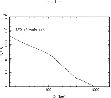
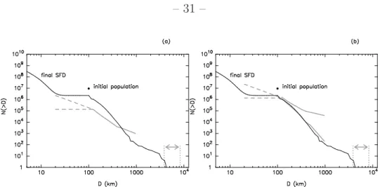
ii) The SFD experienced a significant change in slope to shallower power law values near D ∼ 100 km. This left a “bump” that can still be seen in the current main belt SFD (Fig. 1).
iii) The number of D = 100-1,000 km objects was much larger than in the current population, probably by a factor of 100 to 1,000
iv) The main belt included 0.01-0.1 Earth mass (M⊕) planetary embryos.
Below, we discuss how we obtained properties (i)–(iv) of the reconstructed post-accretion asteroid belt (the expert reader can skip directly to sect. 3). We are confident that the reconstructed belt is a reasonable approximation of reality because it was worked out within the confines of a comprehensive model that not only explains the major properties of the observed asteroid belt but also those of the terrestrial planets (Petit et al., 2001; O’Brien et al., 2007). Therefore, we argue it is reasonable to use the reconstructed belt to test predictions from planetary accretion simulations.
2.1. The current size distribution of the main asteroid belt
The observed SFD of main belt asteroids is shown in Fig. 1. The asteroid population throughout the main belt is thought to be complete down to sizes of at least 15 km in diameter, possibly even 6-10 km (Jedicke et al., 2002; Jedicke, personal comm.). Thus, the SFD above this size threshold is the real asteroid SFD.
2.2. The mass deficit of the main asteroid belt
An estimate of the total mass of the main asteroid belt can be obtained from the above SFD, where the largest asteroids have known masses (Britt et al., 2002), and from an analysis of the motion of Mars, which constrains the contribution of asteroids too small to be observed individually (Krasinsky et al., 2002). The result is ∼ 6 × 10⁻⁴ Earth masses or
3.6 × 1024g. As we argue below, this mass is tiny compared to the mass of solids that had
to exist in the main belt region at the time of asteroid formation. The primordial mass of the main belt region can be estimated by following several different lines of modeling work.
First, we consider the concept of the so-called minimum mass solar nebula (MMSN; Weidenschilling, 1977; Hayashi, 1981). The MMSN implies the existence of 1-2.5 Earth masses of solid material between 2 and 3 AU. Accordingly, this means that the main belt region is deficient in mass by a factor 1,500-4,000. Using the same procedure, Mars’ region also appears deficient in mass, though only by a factor of ∼ 10. We stress that these depletion factors are actually lower bounds because they are estimated using the concept of the minimum mass solar nebula.
Second, we can consider estimates of the mass of solids needed in the main belt region for large asteroids to accrete within the time constraints provided by meteorite data, e.g. within a few million years (Scott, 2006). Published results from different accretion models, i.e. those using collisional coagulation (e.g. Wetherill, 1989) or gravitational instability (Johansen et al., 2007) consistently find that several Earth masses of material in the main belt region were needed to make Ceres-sized bodies within a few My. Thus, it seems unlikely that the current asteroids were formed in a mass-deficient environment.
Third, models of chondrule formation that assume they formed in shock waves (Connolly and Love, 1998; Desch and Connolly, 2002; Ciesla and Hood, 2002) require a surface density of the disk (gas plus solids) at 2.5 AU of ∼ 3,000 g/cm2, give or take a
Fig. 1.— The size-frequency distribution (SFD) of main belt asteroids for D > 15 km, assuming, for simplicity, an albedo of pv = 0.092 for all asteroids. According to Jedicke et al. (2002),
D > 15 km is a conservative limit for observational completeness.
factor of 3. Assuming a gas/solid mass ratio of ∼ 200 in the main belt region, this value would correspond to a mass of solids of at least 3 Earth masses between 2 and 3 AU.
Therefore, the available evidence is consistent with the idea that the asteroid belt has lost more than 99.9% of its primordial mass. This makes the current mass deficit in the main belt larger than a factor of 1,000, with probable values between 2,000 and 6,000.
2.3. Can collisions create the mass deficit found in the main belt region?
If so much mass once existed in the primordial main belt region, collisional evolution, dynamical removal processes, or some combination of the two were needed to get rid of it and ultimately produce the current main belt population. Here we list several arguments describing why the mass depletion was unlikely to have come from collisional evolution of the main belt SFD.
1: Constraints from Vesta
The asteroid (4) Vesta is a D = 529 ± 10 km differentiated body in the inner main belt with a 25-40 km basaltic crust and one D = 460 km impact basin at its surface (Thomas et al., 1997). Using a collisional evolution model, and assuming various size distributions consistent with classical collisional coagulation scenarios, Davis et al. (1985) showed that the survival of Vesta’s crust could only have occurred if the asteroid belt population was only modestly larger than it is today at the time the mean collision velocities were pumped up to ∼ 5km/s (i.e. the current mean impact velocity in the main belt region; Bottke et al. 1994). Another constraint comes from Vesta’s basin which formed from the impact of a D ∼ 35 km projectile (Thomas et al., 1997). The singular nature of this crater means that Vesta, and the asteroid belt in general, could not have been repeatedly bombarded by large (i.e. ∼ 30 km-sized) impactors; otherwise, Vesta should show signs of additional basins (Bottke et al., 2005a, 2005b; O’Brien and Greenberg, 2005). More specifically, given the current collision probabilities and relative velocities among objects of the asteroid belt, the existence of one basin is consistent with the presence of ∼ 1000 bodies with D > 35 km (i.e. the current number; see Fig. 1) over the last ∼ 4 Gy. The constraints describing Vestas limited collisional activity apply from the time when the asteroid belt acquired an orbital excitation (i.e. eccentricity and inclination distributions) comparable to the current one.
2: Constraints from asteroid satellites
Collisional activity among the largest asteroids in the main belt is also constrained by the presence of collisionally-generated satellites (called SMATS; Durda et al., 2004). Observations indicate that ∼ 2% of D > 140 km asteroids have SMATS (Merline et al., 2002; Durda et al., 2004). It was shown in Durda et al. (2004) that this fraction is consistent, within a factor of 2–3, with the collisional activity that the current asteroid belt population has suffered over the last 4 Gy. If much more collisional activity had taken
place, as required by a collisional grinding scenario, one should also explain why so few SMATS are found among the D > 140 km asteroids. Like above, this constraint applies since the time when the asteroid belt acquired the current orbital excitation.
3: Constraints from meteorite shock ages
We also consider meteorite shock degassing ages recorded using the 39Ar-40Ar system.
Many stony meteorite classes (e.g. L and H-chondrites; HEDs, mesosiderites; ureilites) show evidence that the surfaces of their parent bodies were shocked, heated, and partially degassed by large and/or highly energetic impact events between ∼ 3.5-4.0 Gy ago, the time of the so-called ‘Late Heavy Bombardment’ (e.g. Bogard, 1995; Kring and Swindle, 2008). Many meteorite classes also show evidence for Ar-Ar degassing events on their parent body at 4.5 Gy, a time when many asteroids were experiencing metamorphism or melting. Curiously, the evidence for shock degassing events in the interim between 4.1-4.4 Gy is limited, particularly when one considers that this is the time when the asteroid belt population was expected to be ∼ 10 times more populous than it is today (Gomes et al., 2005; Strom et al., 2005). It is possible we are looking at a biased record. For example, because shock degassing ages only record the last resetting event that occurred on the meteorite’s immediate precursor, impacts produced by projectiles over the last 4.0 Gy may have erased radiometric age evidence for asteroid-asteroid impacts that occurred more than 4.0 Gy. On the other hand, many meteorite classes show clear evidence for events that occurred 4.5 Gy. Why did the putative erasure events fail to eliminate these ancient Ar-Ar signatures? While uncertainties remain, the simplest explanation is that the main belt population experienced a minimal amount of collisional evolution between 4.1-4.5 Gy. Thus, meteorites constrain the main belt regions overall collisional activity from the time when impacts among planetesimals became energetic enough to produce shock degassing.
excitation experienced only a moderate amount of net collisional activity over its lifetime. Using numerical simulations, Bottke et al. (2005a,b) found it to be roughly the equivalent of ∼ 10 Gy of collisional activity in the current main belt. It is unlikely that this limited degree of collisional activity could cause significant mass loss. In fact, the current dust production rate of the asteroid belt is at most 1014 g yr−1 (i.e. assuming all IDPs come from
the asteroids; Mann et al., 1996). Thus, over a 10 Gy-equivalent of its present collisional activity, the asteroid belt would have lost 1024 g only 1/3 of the current asteroid belts mass
and a negligible amount with respect to its inferred primordial mass of ∼ 1028 g.
If collisions since the orbital excitation time cannot explain the mass deficit of the asteroid belt, then the mass either had to be lost early on, when collisions occurred at low velocities, or by some kind of dynamical depletion mechanism. In the first case, only small bodies could be collisionally eroded, given the low velocities. Even in the “classical” scenario, where the initial planetesimal population was dominated by km-size bodies, it is unlikely that more than 90% of the initial mass could be lost in this manner, particularly because these bodies had to accrete each other to produce the larger asteroids observed today. We will check this assertion in sect. 3. Accordingly, and remembering that the total mass deficit exceeds 1,000, 99% (or more!) of the remaining main belt’s mass had to be lost by dynamical depletion, defined here as a a process that excited the eccentricities of a substantial fraction of the main belt population up to planet-crossing values. These excited bodies would then have been rapidly eliminated by collisions with the planets, with the Sun, or ejection from the Solar System via a close encounter with Jupiter. We describe in sect. 2.5 the most likely process that produced this depletion and its implications on the total number of objects and size distribution of the “post-accretion asteroid belt”.
2.4. Constraints provided by the main belt size distribution
The limited amount of collisional grinding that has taken place among D > 100 km bodies in the asteroid belt has two additional and profound implications. The size distribution of objects larger than 100 km could not have significantly changed since the end of accretion (Davis et al., 1985; Durda et al., 1998; Bottke et al., 2005, 2005b, O’Brien and Greenberg 2005). This means the observed SFD for D > 100 km is a primordial signature or “fossil” of the accretional process. This characterizes property (i) of the post-accretion
main belt population.
Moreover, it was shown that the “bump” in the observed SFD at D = 100 km (see Fig. 1) is unlikely to be a by-product of collisional evolution. Bottke et al. (2005, 2005b) tested this idea by tracking what would happen to an initial main belt SFD whose power law slope for D > 100 km bodies was the same for D < 100 km bodies. Using a range of disruption scaling laws, they found they could not grind away large numbers of D = 50-100 km bodies without producing noticeable damage to the main belt SFD at larger sizes (D = 100-400 km) that would be readily observable today. Other consequences include the following. First, they found that large numbers of D ∼ 35 km objects would produce multiple mega-basin-forming events on Vesta. This is not observed. Second, the disruption scaling laws needed to eliminate numerous 50-100 km asteroids would produce, over the last 3.5 Gy, far more asteroid families from 100-200 km objects than the 20 or so current families that are observed. Also, the ratio between the numbers of families with progenitors larger than 100 and 200 km respectively would be a factor of ∼ 4 larger than observed (O’Brien and Greenberg, 2005). Finally, the asteroid belt population, and therefore the NEO population that is sustained by the main belt, would have decayed by more than a factor of 2 over the last 3 Gy (Davis et al., 2002). This is not observed in any chronology of lunar craters (e.g. Grieve and Shoemaker, 1994).
While Bottke et al. (2005, 2005b) could not identify the exact power-law slope of the post-accretional SFD for D < 100 km objects, their model results did suggest that it could not be steeper than what is currently observed. This sets property (ii) of the post-accretion
main belt population. The power-law slope for D < 100 km could have been exceedingly
shallow, with the observed SFD derived from generations of collisional debris whose precursors were fragments derived from break-up events among D > 100 km asteroids. For this reason, in Fig. 3 and all subsequent figures, we bracket the possible slopes of the post-accretion SFD for D < 100 km by two gray lines: the slanted one representing the current slope and the horizontal one representing an extreme case where no bodies existed immediately below 100 km.
2.5. The dynamical depletion of the main belt population
We now further explore property (iii) of the post-accretion main belt, namely the putative dynamical depletion event that should have removed most (i.e. more than 99% in mass) of the large asteroids as required by (a) the current total mass deficit of the asteroid belt (a factor of at least 1,000) and (b) the relatively small mass depletion factor that could have occurred via collisional grinding of small bodies before the dynamical excitation event (at most a factor of 10). So far, the best model that explains the properties of the asteroid belt is the “indigenous embryos model” (Wetherill, 1992; Petit et al., 2001; O’Brien et al., 2007). Other models have been proposed (see Petit et al. (2002), for a review) but all have problems in reproducing at least some of the constraints, so we ignore them here and detail briefly only the indigenous embryos model below.
According to this model (Wetherill, 1992), planetary embryos formed not only in the terrestrial planet region but also in the asteroid belt. The combination of their mutual perturbations and of the dynamical action of resonances with Jupiter eventually removed
them from the asteroid belt (Chambers and Wetherill, 2001; O’Brien et al., 2006). Before leaving the belt, however, the embryos scattered the asteroids around them. This excited the asteroids’ eccentricities and inclinations but also forced the asteroids to random-walk in semi-major axis. As a consequence of their mobility in semi-major axis, many asteroids fell, at least temporarily, into resonance with Jupiter, where their orbital eccentricities and inclinations increased further. By this process, 99% of the asteroids acquired an eccentricity that exceeded the value characterizing the stability boundary of the current asteroid belt (O’Brien et al., 2007). Thus, their fate was sealed and these objects were removed during or after the formation of the terrestrial planets.
In addition, about 90–95% of the asteroids that survived this first stage should have been removed by sweeping secular resonances due to a sudden burst of radial migration of the giant planets that likely triggered the so-called “Late Heavy Bombardment” of the Moon and the terrestrial planets (Gomes et al., 2005; Strom et al., 2005; Minton and Malhotra, 2009). This brings the dynamical depletion factor of the asteroid belt to a total of ∼1,000. However, given the uncertainties in dynamical models and considering that early collisional grinding among small bodies might have removed some fraction of the initial mass, a dynamical depletion factor of ∼ 100 cannot be excluded. It is unlikely that the dynamical depletion factor could be smaller than this.
Large-scale dynamical depletion mechanisms are size independent. Thus, a mass depletion factor of ∼ 1,000 (100) implies that the number of asteroids at the end of the accretion process had to be, on average, ∼1,000 (100) times the current number for all asteroid sizes. This is used to set property (iii) of the post-accretion main belt.
At large asteroid sizes, we are affected somewhat by small number statistics. For instance, assuming a dynamical depletion factor of 1,000, the existence of one Ceres-size body might imply the existence of 1,000 bodies of this size, but is also consistent, at the
10% level, with the existence of only 100 of these bodies.
More precisely, given a population of N bodies, each of which has a probability p to survive, the probability to have M specimen in the surviving population is
P = (1 − p)N −MpMN!/[M!(N − M)!] . (1)
From this, assuming that p = 10−3
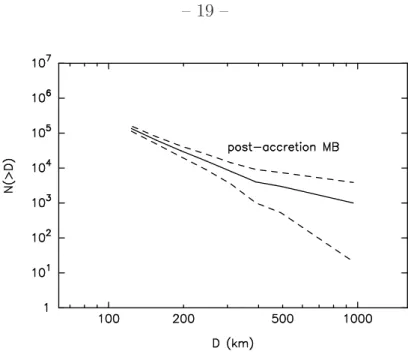
, one can rule out at the 2-σ level that the population of Ceres-size bodies contained less than 21 objects, because otherwise the odds of having one surviving object today would be less than 2.1%. Similarly, we can rule out the existence of more than 3876 Ceres-size objects in the original population, otherwise the odds of having only one Ceres today would be smaller than 2.1%. In an analog way, for the population of bodies with D > 450 km (3 objects today), the 2-σ lower and upper bounds on the initial population are 527 and 7441 objects, respectively. Fig. 2 shows the cumulative SFD of the reconstructed asteroid belt in the 100-1,000 km range (the current SFD scaled up by a factor 1,000; solid curve) and the 2-σ lower and upper bounds computed for each size as explained above (dashed lines). The meaning of this plot is the following: consider all the SFDs that could generate the current SFD via a random selection of 1 object every 1,000; then 95.8% of them fall within the envelope bounded by the dashed curves in Fig. 2. We have checked this result by generating these SFDs with a simple Monte-Carlo code.
We have also introduced a functional norm for these SFDs, defined as
D =X
Di
| log(N′
(> Di)/N(> Di))| , (2)
where Di are the size bins between 100 and 1,000 km over which the cumulative SFD is
computed (8 values), N(> Di) is the current cumulative SFD scaled up by a factor 1,000
and N′
(> Di) is a cumulative SFD generated in the MonteCarlo code. We have found that
95.8% of the MonteCarlo-generated SFDs have D < 6.14. By repeating the MonteCarlo experiment with different (large) decimation factors p we have also checked that the value
Fig. 2.— The size-frequency distribution (SFD) in the 100-1,000 km range, expected for the main belt at the end of the accretion process (e.g. for the reconstructed belt), assuming a dynamical depletion factor of 1,000. The solid line is obtained scaling the current SFD (Fig. 1) by a factor 1,000; the dashed lines show the 2-σ lower and upper bounds, given the current number of objects. The shape of these curves does not change (basically) with the dynamical depletion factor 1/p; the curves simply shift along the y-axis by a quantity log((1/p)/1000).
of D is basically independent on p, while all the curves in Fig. 2 shift along the y-axis proportionally to p (so that the solid line coincides with the current SFD, scaled up by a factor 1/p). These results will be used when testing some of our model results in section 4 and 5.
The embryos-in-the-asteroid-belt-model in Wetherill (1992) does not only explain the depletion of the asteroid belt but also the final orbital excitation of eccentricities and inclinations of the surviving asteroids and the radial mixing of bodies of different taxonomic types (Petit et al., 2001). In addition, it provides a formidable mechanism to explain the delivery of water to the Earth (Morbidelli et al., 2000; Raymond et al., 2004, 2007).
and physical properties of the asteroid belt within the larger framework of terrestrial planet accretion. To date, it is the only model capable of doing so. Thus, if we trust this model, embryos of at least one lunar mass had to exist in the primordial asteroid belt. This
characterizes property (iv) of the post-accretion main belt population. A successful accretion
simulation should not only be able to form asteroid-size bodies in the main belt, but also a significant number of these embryos.
3. The classical scenario: accretion from kilometer-size planetesimals
We start our investigation by simulating the classical version of Step 2 of the accretion process. In other words, we assume that kilometer-size planetesimals managed to form in Step 1, despite the meter-size barrier; the accretion of larger bodies occurrs in Step 2, by pair-wise collisional coagulation. We simulate this second step using our code Boulder. The simulations account for eccentricity e and inclination i excitation due to mutual planetesimal perturbations as well as (e, i) damping due to dynamical friction, gas drag and mutual collisions. Collisions are either accretional or disruptive depending on the sizes of projectiles/targets and their collision velocities.The disruption scaling law used in our simulations, defined by the specific dispersion energy function Q∗
D, is the one provided by
the numerical hydro-code simulations of Benz and Asphaug (1999) for undamaged spherical basaltic targets at impact speeds of 5km/s. See the electronic supplement for the details of the algorithm. However, in section 3.4, we will examine what happens if we use a Q∗
D function that allows D < 100 km disruption events to occur much more easily than
suggested by Benz and Asphaug (1999), as argued in Leinhardt and Stewart (2009) and Stewart and Leinhardt (2009).
Here, and in all other simulations (unless otherwise specified), we start with a total of 1.6 M⊕ in planetesimals within an annulus between 2-3 AU. By assuming a nominal
gas/solid mass ratio of 200, this corresponds to the Minimum Mass Solar Nebula as defined in Hayashi (1981). The bulk mass density of the planetesimals is set to 2 g/cm3, the average
value between those measured for S-type and C-type asteroids (Britt et al., 2002). The simulations cover a time-span of 3 My, consistent with the mean lifetime of proto-planetary disks (Haisch et al., 2001) and hence the probable formation timescale of Jupiter. The initial velocity dispersion of the planetesimals is assumed to be equal to their Hill speed (i.e. vorb[Mobj/(3M⊙)]1/3, where vorb is the orbital speed of the object, Mobj is its mass, and
M⊙ is the solar mass). The lower size limit of planetesimals tracked in our simulation is
diameter D = 0.1 km. Objects smaller than this size are removed from the simulation. We record the total amount of mass removed in this manner and, for brevity, refer to it as dust.
The initial size of the planetesimals is assumed to be D = 2 km. In this simulation, the total mass lost into dust by collisional grinding is 7.45 × 1027 g, i.e. more than one
Earth mass but only 76% of the original mass. This is consistent with our claim in section 2 that, even starting with km-size planetesimals, low-velocity collisions cannot deplete more than 90% of the initial mass.
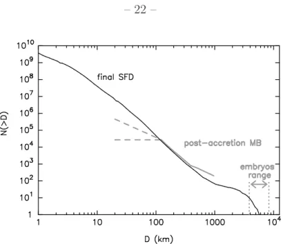
The final SFD of the objects produced in the simulation is illustrated by the black curve in Fig. 3. We find this SFD does not reproduce the turnover to a shallower slope that the post accretion asteroid belt had to have at D ∼ 100 km (i.e. property (ii) of the reconstructed belt). Moreover, in the final SFD shown in Fig. 3, there are about 1.25 million bodies with D > 35 km. Even if we were to magically reduce this population instantaneously by a factor 200, in order to reduce the number of D > 100km bodies to the current number, we would still have ∼ 6, 200D > 35 km objects remaining in the system. Recall (section 2) that D ∼ 35 km projectiles can form mega-basins on Vesta and that the formation of a single basin is consistent with the existence of 1,000 of these objects in the main belt over 4 Gy. Thus, 6,200 objects would statistically produce 6 basins; the
Fig. 3.— The gray lines show the reconstructed (i.e., post-accretion) main belt SFD. The solid gray curve shows the observed main belt SFD for 100 < D < 1, 000 km asteroids scaled up 200 times, so that the number of bodies with D > 100km matches that produced in the simulation. The dashed lines show the upper and lower bound of the main belt power law slope in the 20-100 km range (Bottke et al., 2005). The upper bound corresponds to the current SFD slope. The vertical dotted lines show the sizes of Lunar/Martian-sized objects for bulk density 2 g cm−3. These size
embryos are assumed to have formed across the inner Solar System (Wetherill, 1992; O’Brien et al., 2007). The black curve shows the final SFD, starting from 1.2 × 10¹² planetesimals with D = 2 km,
at the end of the 3 My coagulation/grinding process.
probability that only one mega-basin would form, according to formula (1), is only 1.2%.
For all these reasons, we think that this simulation produces a result that is inconsistent with the properties of the asteroid belt. To test whether these results are robust, we performed additional simulations as detailed below.
3.1. Extending the simulation timescale
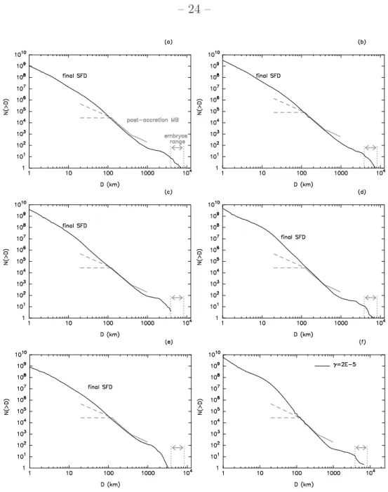
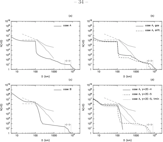
One poorly understood issue is how long the accretion phase should last, i.e. the required length of our simulations. Thus, we continued the simulation presented above up to 10 My. The result is illustrated in Fig. 4a. We find that the total amount of mass lost into dust increases only moderately, reaching at 10 My 78% of the mass at t = 0. Also, SFD does not significantly change between 3 and 10 My. The size of the largest embryos does grow from slightly less than 6,000 km to about 7,000 km, mostly by agglomerating objects smaller than a few tens of kilometers. Accretion and collisional erosion reduce the cumulative number of D > 1 km objects from 3.5 × 10⁹ to 9.3 × 10⁸. For the size range
80 < D <5,000 km, however, the SFD remains identical. So, the mismatch with the “bump” observed at D ∼ 100km does not improve. The number of D > 35km objects decreases slightly relative to Fig. 3; but the probability that only one basin is formed on Vesta in case of an instantaneous dynamical depletion event remains low (5%).
3.2. Changing the initial mass
Another poorly-constrained parameter is the initial total mass of the planetesimal population. For this reason, we tested a range of options. Here we discuss a simulation starting with a system of planetesimals carrying cumulatively 5 M⊕ instead of 1.6 M⊕
as in Fig. 3. This total mass is of the order but slightly larger than that computed in Weidenschilling (1977) and is the same as assumed in Wetherill (1989). The result is shown in Fig. 4b. As a result of the factor of ∼ 3 increase in initial total mass, the final SFD is similar to that of Fig. 3, but scaled up by a factor of ∼ 3 and is nearly indistinguishable in shape for 70 < D <1,000 km objects.
Fig. 4.— As in Fig. 3, but for additional simulations. (a) Continuation of the simulation of Fig. 3 up to 10 My. (b) Starting with 5 M⊕ of D = 2 km planetesimals (here the solid gray line reproduces the current SFD scaled up by a factor 600, instead of 200 as in all other panels). (c) Starting with 1.6 M⊕of D = 600 m planetesimals. (d) Starting with 1.6 M⊕ of D = 6 km planetesimals. (e) Assuming that Q∗D is 1/8 of the value given in Benz and Asphaug for ice. (f) Introducing turbulent scattering with γ = 2 × 10⁻⁵(a run with γ = 2 × 10⁻⁴ resulted in basically no accretion). See text for comments on these results.
Thus, the turn-over of the SFD at D ∼ 100 km is still not reproduced. As a consequence, there are about 2.5 million bodies with D > 35 km, the putative size of the
basin-forming projectile on Vesta. Invoking an instantaneous dynamical depletion event capable of removing a factor of 600 from the population, a value needed to reduce the the number of D > 100km bodies to the current number, about 4,000 D > 35 km objects would be left in the system. Thus, about 4 basins should have formed on Vesta; the probability that only 1 would have formed, according to (1) is 6%.
For all these reasons, we think that it would be very difficult to claim that the simulation of Fig. 4b is successful. Notice that also in this case the total amount of mass lost in collisional grinding does not exceed 86% of the initial mass.
3.3. Changing the initial size of the first planetesimals
Fig. 4c and 4d illustrate how the results depend on the size of the initial planetesimals. The simulation in Fig. 4c starts from 1.6 M⊕ of material in D = 600 m planetesimals
instead of D = 2 km as in the nominal simulation. The final SFD is indistinguishable from that of the nominal simulation up to D ∼ 3,000 km. Instead, there is a deficit of larger planetary embryos.
The simulation in Fig. 4d starts from the same total mass in the form of D = 6 km planetesimals. The final SFD has an excess of 10-200 km objects relative to the SFD in the nominal simulation, but the SFDs are similar in the D = 40-4,000 km range.
Thus, these cases can be rejected according to the same criteria applied in Sec. 3.2 .
3.4. Changing the specific dispersion energy of planetesimals
In the previous simulations we assumed that the planetesimals have size-dependent specific disruption energy (Q∗
several km/s (see Benz and Asphaug, 1999). Leinhardt and Stewart (2009) have argued that the original planetesimals might have been weak aggregates with little strength. Moreover, Stewart and Leinhardt (2009) showed that early planetesimals should have low Q∗
D also because impact energy couples to the target object better at low velocities. In
these conditions, Q∗
D might be more than an order of magnitude weaker than the one that
we adopted at all sizes. To test how the results change for extremely weak material, we have re-run the coagulation simulation starting with 1.6 M⊕ in D = 2km planetesimals
(that of Fig. 3), this time assuming Q∗
D is one eighth of that reported by Benz and Asphaug
(1999) for competent ice struck at impact velocities of 1km/s. This is fairly close to the value found by Leinhardt and Stewart (2009) for strenghtless planetesimals.
The resulting SFD is shown in Fig. 4e. Overall, the outcome is not very different from that of the nominal simulation. Despite of the weakness of the objects, the total mass lost in collisional grinding (8.4 × 1027g) does not exceed 90% of the initial mass, as we argued in
section 2. Interestingly, though, this simulation fails to form objects more massive than our Moon. Thus, in conclusion, the change to a new disruption scaling law produces a worse fit to the constraints than before, particularly because constraint (iv) of the reconstructed belt (e.g. the existence of Lunar-to-Martian mass embryos) is not fulfilled.
3.5. The effect of turbulence
In all previous simulations we have implicitly assumed that the gas disk in which the planetesimals evolve is laminar. Thus, the gas can only damp the velocity dispersion of the planetesimals. In this case, the sole mechanism enhancing the planetesimal velocity dispersion is provided by mutual close encounters, also named viscous stirring (Wetherill and Stewart, 1989; see section. 1.4.1 of the electronic supplement). In reality, the disk should be turbulent at some level. As discussed in Cuzzi and Weidenschilling (2006), local
turbulence contributes by stirring the particles and increasing their velocity dispersion. This effect is maximized for meter-sized objects. In addition, however, turbulent disks show large-scale fluctuations in gas density (Papaloizou and Nelson, 2003). The fluctuating density maxima act as gravitational scatterers on the planetesimals, providing an additional mechanism of excitation for the velocity dispersion that is independent of the planetesimal masses (Nelson et al., 2005). To distinguish this mechanism from that discussed by Cuzzi and Weidenschilling, we call it turbulent scattering hereafter. Ida et al. (2008) showed with simple semi-analytical considerations that turbulent scattering can be a bottleneck for collisional coagulation because it can move collisions from the accretional regime to the disruptive regime. Here, we check this result with our code.
Boulder accounts for turbulent scattering using the recipe described in Ida et al. (2008) and detailed in sect. 1.4.7 of the electronic supplement of this paper. In short, in the equations for the evolution of the velocity dispersion, there is a parameter γ governing “turbulence strength”. The effective value of γ in disks that are turbulent due to the magneto-rotational instability is uncertain by at least an order of magnitude. Simulation by Laughlin et al. (2004) suggest that γ ∼ 10−3
–10−2
, but values as low as 10−4
cannot be excluded (Ida et al., 2008). The relationship between γ and the more popular parameter α that governs the viscosity in the disk in the Shakura and Sunyaev (1973) description has been recently investigated in details by Baruteau (2009). He found that α ∝ γ2/(h/a)2
where h/a is the scale-height of the gas disk; for h/a = 3%, γ = 10−4 corresponds to
α ∼ 5 × 10⁻⁴.
We have re-run the coagulation simulation of Fig. 3, assuming γ = 2 × 10⁻⁴ (which
corresponds to α ∼ 2 × 10⁻³ according to Baruteau’s scaling).. In this run we adopt an
initial velocity dispersion of the planetesimals that is larger than that assumed in the non-turbulent simulations illustrated above. Recall that in all previous simulations the
initial velocity dispersion of the objects was set equal to their Hill velocity. These velocities are too small for a turbulent disk. If we adopted them, we would get a spurious initial phase of fast accretion, before the velocities were fully stirred up by the turbulent disk. Thus, we need to start with velocity dispersions that represent the typical values achieved in the disk. More precisely, for D = 2 km objects, we assume initial eccentricities and inclinations that are the equilibrium values obtained by balancing the stirring effect of the turbulent disk with the damping effects due to gas drag and mutual collisions (Ida et al., 2008). We used Boulder to estimate what these values should be by suppressing collisional coagulation/fragmentation and letting the velocity dispersion evolve from initially circular and co-planar orbits. We found that at equilibrium we get e ∼ 2i ∼ 2.5 × 10⁻³. This value
is attained in about 50,000 years, whereas e ∼ 2i ∼ 1.2 × 10⁻³ is attained in 5,500 years.
In the simulation performed with this set-up, growth is fully aborted. The largest planetesimals produced in 3 My are just 2.5 kilometer in diameter, whereas 9.58 × 1027g are
lost in dust due to collisional grinding. This result is due to the fact that collisions become rare (because the gravitational focussing factor is reduced to unity by the enhanced velocity dispersion) and barely accretional even for “strong” Q∗
D disruption functions that is used in
this simulation (for basaltic targets hit at 5km/s; Benz and Asphaug, 1999). We also ran a simulation where we did not modify the initial velocity dispersion of the planetesimals, although we consider this unrealistic for the reasons explained above. In this case there is a short initial phase of growth, as expected, which rapidly shuts off; the largest objects produced have D = 40km. These results confirm the analysis of Ida et al. (2008); accretion is impossible in turbulent disks if all planetesimals are small.
To investigate how weak “turbulence strength” should be to allow accretion from D = 1 km planetesimals, we also ran a simulation assuming γ = 2 × 10⁻⁵. In this case,
corresponds to α ∼ 2 × 10⁻⁵, that is well below a minimum reasonable value in a turbulent
disk; however, it might be acceptable for a dead zone, e.g. a region of the disk where the magneto-rotational instability is not at work. The solid curve in Fig. 4f shows the final SFD in this simulation. It now looks similar to that obtained in the nominal simulation of Fig. 3, which had no turbulent scattering. Thus, this very low level of turbulence does not inhibit growth, but like the nominal simulation in Fig. 3, the resulting SFD is inconsistent with that of the reconstructed main belt.
3.6. Conclusions on the classical scenario
From the simulations illustrated in this section, we conclude that the SFD of the initial planetesimals were not dominated by objects with sizes the order of one kilometer. In fact, in a turbulent disk, 1 km planetesimals would not have coagulated to form larger bodies. In a dead zone, collisional coagulation would have produced a final SFD that is inconsistent with the current SFD in the main asteroid belt because the bump at D ∼ 100 km is not reproduced; also we find it unlikely (at the few percent level) that only one big basin formed on Vesta with such a SFD, even in the case of an instantaneous dynamical depletion event of the appropriate magnitude. While we were writing the final revisions of this paper, we became aware that Weidenschilling (2009) reached the same conclusions with similar non-turbulent simulations performed with a different code.
Obviously, there is an enormous parameter space left to explore, and -strictly speaking- an infinite number of simulations would be necessary to prove that the SFD of the reconstructed post-accretion main belt is incompatible with the classical collisional accretion model starting from km-size planetesimals. Nevertheless, we believe that the 9 simulations presented above are sufficient enough to argue that our result is reasonably robust.
Given this conclusion, in the next sections we try to constrain which initial planetesimal SFD would lead, at the end of Step 2, to the SFD of the reconstructed main belt.
4. Accretion from 100 km planetesimals
We start our search for the optimal initial planetesimal SFD by assuming that all planetesimals originally had D = 100 km. Note that no formation model predicts that the initial planetesimals had to have the same size. We make this assumption as a test case to probe the signature left behind in the final SFD by the initial size of the objects. More specifically, we attempt to satisfy property (ii), the turnover of the size distribution at D ∼ 100 km, assuming that this might be the signature of the minimal size of the initial planetesimals.
As before, our input planetesimal population carries cumulatively 1.6 M⊕. This implies
that there are initially 9.4 × 10⁶ planetesimals. The coagulation simulation covers a 3 My
time-span. No turbulent scattering is applied.
The final SFD is shown in Fig. 5a (solid curve). This SFD has the same properties of that obtained by Weidenschilling (2009) starting from D = 50km planetesimals. A sharp turnover of the SFD is observed at the initial planetesimal size. This is in agreement with the observed “bump” (i.e. property (ii) of the reconstructed belt). However, the final SFD is much steeper than the SFD of the current asteroid belt. Nevertheless, it would be premature to consider this simulation unsuccessful because we showed in Fig. 2 that the slope of the SFD of the reconstructed asteroid belt has a large uncertainty. Thus, in Fig. 5b, we replot the final SFD against the 2-σ bounds of the reconstructed main belt SFD. These bounds have been taken from Fig. 2 and are “scaled up” by a factor of 10 so that they match the total number of D > 100 km objects found in the simulation. As one
Fig. 5.— (a): Non-turbulent simulation starting with 1.6 M⊕ in D = 100 km objects. The bullet
shows the initial size and total number of planetesimals. The black curve reports the final SFD obtained after 3 My of collisional coagulation. The grey lines sketch the reconstructed asteroid belt SFD as in Figs. 3 and 4. (b): like panel (a), but in this case the grey solid lines report the 2-σ bounds of the SFD of the reconstructed asteroid belt, from Fig. 2. Moreover, all grey lines have been moved upwards by a factor of 10, to match the number of D > 100km objects in the SFD resulting from the simulation.
can see, the final SFD falls slightly out of the lower bound of the reconstructed SFD. This means that the result is inconsistent, at 2-σ, with the data (i.e. with the current SFD).
Another way to check the statistical match between the simulation SFD and the reconstructed main belt SFD is through the parameter D defined in (2). The SFD resulting from this simulation has D = 8.20; only 0.5% of the SFDs generated from the current SFD in a Monte-Carlo code have D larger than this number. Thus, we can actually reject the result of this simulation as inconsistent with the reconstructed main belt at nearly the 3-σ level.
Rejecting this simulation, however, is not enough to exclude the possibility that the initial planetesimals were ∼ 100 km in size. Before accepting this conclusion, we need to more extensively explore parameter space. The simulation reported in Fig. 5 is indeed simplistic because it did not account for the effects of turbulence in the disk. Recall,
however, that the works that motivated us to start with large planetesimals (Johansen et al., 2007; Cuzzi et al., 2008) assumed (and required) a turbulent disk, so we need to cope with turbulence effects. Turbulence should affect our simulation in two respects: (I) theoretical considerations (Cuzzi et al., 2008) indicate that planetesimals should form sporadically over the lifetime of the gas disk, in qualitative agreement with meteorite data (Scott, 2006), whereas in the previous simulation we introduced all the planetesimals at t = 0; (II) turbulent scattering should enhance the velocity dispersion of the planetesimals, as we have seen in sect. 3.5.. With a new suite of more sophisticated simulations, we now attempt to circumvent our model simplifications. We do this in steps, first addressing issue (I), still in the framework of a laminar disk, and then (II).
To account for (I), we randomly introduce planetesimals in Boulder over a 2 My time-span in two different ways. In case-A, we assume all the mass was initially in small bodies. Every time a 100-km planetesimal is injected in the simulation, we remove an equal amount of mass from the small bodies. In case-B, we inject equal mass proportions of small bodies and planetesimals. This second case mimics the possibility that planetesimal formation is regulated by the availability of ‘building blocks’. Note that chondrules may be such building blocks; they are an essential component of many meteorites and they appear to have formed progressively over time (Scott, 2006). In both cases, we model the small body population with D = 2 m particles, which might be considered as tracers, representing a population of smaller bodies of the same total mass (for instance chondrule-size particles in the model of Cuzzi et al., or meter-size boulders in the model of Johansen et al.). In the previous section, bodies of any size accreted or disrupted depending on the impact energy relative to their specific disruption energy, consistent with the classical scenario of planetesimal accretion. Here, we change our prescription. We assume that our small-bodies/tracers do not disrupt or accrete upon mutual collisions. The rationale for this comes from the models of Johansen et al. and Cuzzi et al. and is twofold. First, bodies so
small have difficulty sticking to one other, so that they can not grow by binary collisions; when they form large planetesimals, they do so thanks to their collective gravity. Second, a large number of small bodies have to be in the disk at all times, in order to be able to generate planetesimals over the spread of timescales shown by meteorite data (Scott, 2006). However, the typical relative velocities of the small bodies are not very small, because of the effects of turbulence. Thus, either the small bodies are very strong or, if they break, they must be rapidly regenerated by whatever process formed them from dust grains in first place.
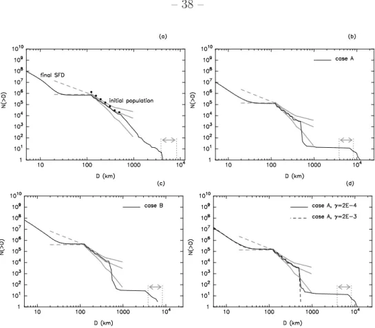
The solid black line in Fig. 6a shows the final SFD obtained in case-A. The availability of small bodies promotes runaway growth among the 100-km planetesimals introduced at early times into the simulation. This leads to very distinctive signatures in the resulting SFD: a steep fall-off above the input size of the planetesimals; the presence of very large planetary embryos; a very shallow slope at moderate sizes (in this case, from slightly more than 100 to several 1,000km) and an overall deficit of objects in this size-range. As a result, the SFD that does not match that of the reconstructed main belt even within the 2-σ boundaries.
For completeness, we present in Fig. 6b two additional variants of this nominal simulation. In one, inspired by the Cuzzi et al. work, we assume that our 2 m-particles are tracers for chondrule-size objects. Chondrules would be strongly coupled with the gas, so we assume, for simplicity sake, that the particles are perfectly coupled with the gas. In practice, instead of letting our particles evolve in velocity space according to the damping/stirring equations of Boulder (as in the nominal simulation), we force them to have the same velocity of the gas (i.e. 60 m/s) relative to Keplerian orbits. The result is illustrated by the black solid curve. In the second variant, inspired by the Johansen et al. work, we assume that our 2 m-particles are tracers for meter-size boulders. These objects should migrate
Fig. 6.— Additional coagulation simulations with 100 km initial planetesimals. The black curves show the final SFDs; the grey lines sketch the reconstructed asteroid belt SFD and its 2-σ bounds as in Figs. 5b. (a) Non-turbulent case-A simulations, where initially all the mass is in D = 2 m particles and the 100 km objects are introduced progressively over 2 My. Here, the velocity dispersion of the 2 m-particles evolves according to the damping (collisional & gas drag) and viscous stirring equations. (b) The same as (a) but with different assumptions on the dynamical evolution of the particles. The dashed curve refers to the case where the radial drift speed of the 2 m particles due to gas drag is also taken into account. The solid curve refers to the case where the particles are assumed to be tracers of much smaller bodies, fully coupled with the gas. (c) Non-turbulent case-B simulation, where equal masses of 2 m-particles and 100km-planetesimals are introduced progressively over 2 My, up to a total of 3.2 M⊕. (d) Case-A simulations where the velocity dispersion of particles and planetesimals is stirred by turbulent scattering. The solid curve is for γ = 2×10⁻⁴, the dashed and dotted curves for γ = 2 × 10⁻⁵; in the case shown by the dotted curve we impose that the minimal eccentricity of the D = 2 m particles cannot decrease below 0.001 and the inclination below 5×10⁻⁴.
very quickly towards the Sun by gas drag. We neglect radial migration in Boulder because the annulus that we consider (2–3 AU) is too narrow. This is equivalent to assuming that
the bodies that leave the annulus through its inner boundary are substituted by new bodies drifting into the annulus through its outer boundary. The drift speed, however, should be included in our calculation of the relative velocities of particles and planetesimals. Accordingly, we add a 100m/s radial component to the velocities of all our tracers. The result is illustrated by the black dashed curve. We find the dashed and solid curves are very similar to the solid curve of panel a. Thus, none of the considered effects appear to have much effect in changing the final SFD. Based on this, we believe it will be reasonable to neglect these corrections to the velocity of our particles in the remaining simulations. This reduces the number of cases to be investigated and simplifies our discussion.
The solid black line in Fig. 6c shows the final SFD obtained in case-B. Again, the signature of runaway growth, triggered by the availability of a large amount of mass in small particles, is highly visible. Consequently, the SFD does not match at all that of the reconstructed main belt. In particular, it shows a strong deficit of 100-1,000 km bodies.
In order to get a better match with the SFD of the main belt, we would need to suppress/reduce the signature of runaway growth. One potential way to do this is to enhance the dispersion velocities of small bodies via turbulent scattering (see sect. 3.5). Thus, we proceed to the inclusion of this effect, which addresses issue (II) mentioned above in this section.
We start by assuming that the parameter γ = 2 × 10⁻⁴ (relatively small compared to
expectations). For the 2 m-particles we assume initial eccentricities and inclinations that are the equilibrium values obtained by balancing the stirring effect of the turbulent disk with the damping effects due to gas drag and mutual collisions (e ∼ 2i ∼ 7 × 10⁻⁵). For
the 100km-planetesimals that are injected in the simulation, we assume that eccentricity and inclination are 1/2 of their equilibrium values (accounting also for tidal damping; Ida et al., 2008). This means e = 0.005 and i = e/2. A simulation of the evolution of the
eccentricity/inclination of a 100 km-planetesimal in a turbulent disk shows that these values are achieved in ∼ 100, 000 y starting from a circular orbit within the disk’s mid-plane. The solid black curve in Fig. 6d shows the result for the case-A simulation with this settings. Even with this small amount of turbulent scattering, the accretion is strongly inhibited and the largest objects do not exceed D = 200 km. In a second simulation, we decreased γ by a factor of 10, as well as the initial eccentricities and inclinations. This makes turbulent scattering so weak that runaway growth turns back on, making the final SFD similar to those shown in panel b. We remark, though, that the initial eccentricity and inclination of the particles are much smaller than what one might expect, due to simple diffusion due to local turbulence (Cuzzi and Weidenschilling, 2006). This might have favored runaway growth. In reality, turbulent diffusion should prevent the eccentricities and inclinations of small bodies to become smaller than e ∼ 2i ∼ 10−3 (Cuzzi, private communication). Thus,
we did a third simulation, still adopting γ = 2 × 10⁻⁵, but imposing that e and i of our
particles/tracers do never decrease below these minimal values. The result is shown by the dotted curve. Runaway growth is now less extreme than in the previous case (the slope of the SFD just above D = 100 km is shallower and the final embryos are smaller), but it is still effective. Again, the final SFD is inconsistent with the asteroid belt constraints. Thus, we conclude that the accretion process in the presence of a large mass of small particles is very sensitive to the effects of turbulent scattering: if turbulent fluctuations are too violent, accretion is shut off; if they are too weak, runaway growth occurs. In both cases, no match can be found for the reconstructed main belt.
We conclude from these simulations that the initial planetesimal SFD had to span a significant range of sizes; our best guess would be upwards from 100 km. In the next two sections we will try to constrain the size (Dmax) of the largest initial planetesimals and the
SFD in the 100 km–Dmax range that are necessary to achieve a final SFD consistent with
5. Accretion from 100–500 km planetesimals
Here we start with planetesimals in the D = 100-500 km diameter range, with an initial SFD whose slope is the same as the one observed in the reconstructed (and current) SFD of the asteroid belt.
In the first simulation, all the planetesimals are input at t = 0, as in the simulation of Fig. 5a. In order to place 1.6 M⊕ in these bodies, we have to assume they were
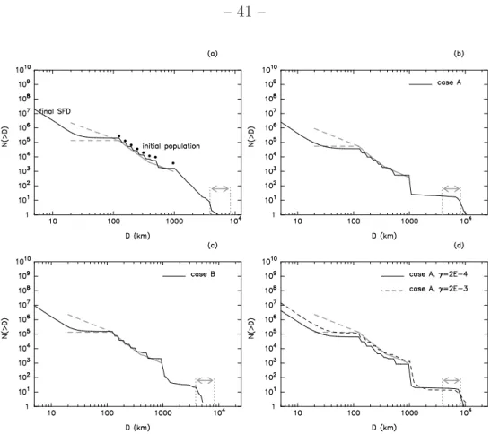
∼ 10, 000 times more numerous than current asteroids in the same size range. As in the previous sections, no turbulent scattering is taken into account in this first simulation. The final SFD is shown in Fig. 7a. An important result is that the slope of the input SFD is preserved to the end of the simulation. The turn-over of the final SFD at D ∼ 100 km is recovered and a few Lunar-mass embryos are produced. Notice, though, that the final SFD shows a sharp break at the initial planetesimals’ maximum size (D > 500 km); for sizes larger than this threshold, the slope is steeper than the initial slope in the 100-500km range. The observed SFD of the asteroid (middle grey solid line in the figure) does not show this behavior. As discussed in section 2, however, the observed SFD is determined by a single object (i.e. Ceres) and therefore the determination of the SFD of the reconstructed belt is affected by small number statistics. With a 95.8% probability, the post-accretion SFD of the asteroid belt should be confined between the upper and lower solid gray curves shown in the figure. We find the final SFD in our simulation does fulfill this requirement very well.
One might be tempted to claim success on the basis of this simulation, but we caution that this run is overly simplistic for the reasons that we enumerated in the previous section: we assumed that (I) all planetesimals are introduced at time = 0 My and (II) turbulent scattering was not taken into account. We lift these approximations below.
A simulation conducted with the case-A set-up discussed in the previous section (Fig. 7b) exacerbates the break of the SFD at D ∼ 500km. This is because the large
Fig. 7.— Like Fig. 6, but starting from initial planetesimals in the 100-500 km range and a main belt-like SFD in this size interval, as shown by the filled dots in panel (a). The three solid gray curves reproduce the reconstructed SFD and its 2-σ bounds (see Fig. 2), rescaled so that the total number of D > 100km objects matches that obtained in each simulation.
planetesimals introduced early in the simulation efficiently gobble up the small bodies and form embryos more massive than Mars via runaway growth. The final SFD is in fact typical of this growth mode (see sect. 4): it shows a steep slope just above the initial size of the planetesimals and a deficit of ∼ 1,000 km objects. The final SFD goes outside of the 2-σ boundaries of the reconstructed belt’s SFD, with only 13 bodies with diameters between 500 and 2,000 km (5 bodies if D is restricted to be larger than 530 km). Given the dynamical depletion factor of 1,000 required to bring the number of D > 100km objects to the current number, the probability that Ceres survived is only 1.3% or 0.5%. Thus, even accounting for small number statistics in the observed asteroid SFD, this simulation is highly unlikely
to reproduce the reconstructed main belt.
The result of a simulation conducted with the case-B set-up discussed in the previous section is shown in Fig. 7c. Again, we see in the final SFD the distinctive signature of runaway growth with a sharp break in the slope of the SFD at D ∼ 500km. Hence, the considerations for the previous run also apply in this case.
The runs accounting for turbulent scattering are shown in Fig. 7d. As in the previous section, all simulations are conducted within the framework of the case-A set-up. The solid curve refers to the simulation where γ = 2 × 10⁻⁴. Unlike the run in Fig. 6d, this value
of turbulence strength does not inhibit accretion in this case, such that the signature of runaway growth is evident in the final SFD (this simulation does not produce a good match to the main belt SFD, as in the cases of panels b and c). We defer to section 6.1 a discussion on which values of γ allow accretion as a function of planetesimal sizes. Conversely, if γ is increased to γ = 2 × 10⁻³, accretion is inhibited and the final SFD above the D = 500 km
drops vertically. As in the previous section, we conclude that the accretion process is very unstable with respect to turbulent scattering: if turbulence is too violent, accretion is shut off; if it is too weak, runaway growth occurs.
Thus, from all our runs, we conclude that it is unlikely that the asteroid belt SFD can be reproduced if we start with planetesimals solely in the 100–500 km size range. Our insights from these runs also suggest that reducing the size of the largest initial planetesimals is only going to make the match more problematic. Thus, we argue that the initial planetesimals had to span the full 100–1,000km range, with a power law slope similar to that of the main belt SFD. In the next section we check whether this initial planetesimal distribution does indeed lead to a final distribution matching all asteroid belt constraints.