Analog Computer Research

(1)

Prof. E. A. Guillemin Prof. R. E. Scott R. M. Beckett J. P. Blake M. M. Cerier N. DeClaris Y. C. Ho F. R. Hultberg L. A. Irish M. S. Macrakis J. L. Perry A. N. Spector T. E. Stern R. J. Szmerda

As in the past, the interests of the group have been divided about equally between the development of analog computer components and the exploration of practical methods of network synthesis.

A. ANALOG COMPUTER DEVELOPMENT 1. Cathode Ray Tube Multiplier

This multiplier works on the principle that the area of a rectangle is proportional to the product of its base times its height. A square pattern is obtained on the face of a

cathode-ray tube by means of a television type of raster. Four separate photomultiplier tubes pick up the light from the four quadrants of the pattern, as shown in Fig. XVIII-1.

The outputs of quadrants ABCD are combined as (A + D) - (B + C). Low-frequency signals E and E are then used to move the raster, and the output voltage is

propor-x y

tional to the product Ex Ey, as can be readily seen from the geometry of the figure. The advantage of this scheme over the one proposed by E. J. Angelo in his doctoral thesis, M. I. T., 1952, is that both channels are separately linear, and feedback can be applied to them.

The major troubles encountered in the experimental device were associated with dc drifts in the external amplifiers.

M. M. Cerier K, E_x

:~i

.

-- I K3

Fig. XVIII- 1

Cathode ray tube multiplier.

Fig. XVIII-2

Inverse trigonometric generator.

~

Y~cr;l

''

Y

(2)

(XVIII. ANALOG COMPUTER RESEARCH)

2. A Square-Law Multiplier

A germanium-diode, square-law device, with a static accuracy of 1 percent and a

bandwidth of 100 kc/sec has been built and tested. An "absolute-value" circuit which

allows four-quadrant operation of a square-law multiplier with only two squaring

cir-cuits has also been built.

J. L. Perry

3. A Probability Multiplier

The probability multiplier uses the mathematical principle that the probability of a

group of independent events occurring simultaneously is equal to the product of the

prob-ability of each event occurring by itself.

Consider a series of similar pulses in which

the period of each pulse is B and the duration of each pulse is A.

The probability of

a pulse occurring at any particular instant is equal to the duty ratio A/B.

Two such

trains of pulses are used, and coincidence between them is detected.

With carrier

pulses at approximately 50 kc/sec, the frequency response is good only to 40 cps.

The

accuracy is approximately 3 percent. The frequency response is the main limitation

of this type of multiplier.

A. N. Spector

4. High-Speed Analog Computer

For a given accuracy of solution the gain required in an analog computer drops as

the solution speed is increased. A first approximation to the theoretical analysis shows

that for an amplifier with a given gain bandwidth product the error is constant

regard-less of the solution time. To test these conclusions an amplifier with a bandwidth of

10 Mc/sec has been constructed and used in a computer with a repetition rate of

1000 cps.

An integrator, designed around this amplifier, had a phase error which was less

than 20 from 1000 cps to more than 100, 000 cps.

The corresponding transient errors

would be in

the neighborhood of 1.

5 percent.

R. M. Beckett

5. Solution of Simultaneous Equations on an Analog Computer

An investigation was conducted on the practicability of solving simultaneous algebraic

equations with a standard analog computer.

The first result of the investigation showed that much more satisfactory operation

could be obtained by using integrators than by using adders.

With integrators the

equa-tions are solved directly by the method of steepest descent.

A second and perhaps more surprising result was concerned with solving matrices

(3)

-84-whose determinants approach zero. It was found experimentally that the percentage of error in the results decreased as the determinant decreased in size, right to the point of instability. This result indicates that machine errors are more important in influ-encing the results than the size of the determinant.

F. R. Hultberg

6. Inverse Trigonometric Function Generator

A device has been built that generates the inverse trigonometric functions of an analog input. The principle used is the measurement of the arc lengths in various quadrants of a circle whose axes are directly dependent on the value of the input. The basic diagram is shown in Fig. XVIII-2. From the geometry it is easily seen that

-

1

x

(1)

#2

+

(3 = 2 cos R and

(91 + 4) - ( + 3) = 4 sin-I y (2)

The circle is obtained by means of a circular sweep on a cathode-ray tube. The arc length is measured by means of the output from two phototubes separated by a partition along the y-axis of the cathode-ray tube.

The accuracy of the first crude device was approximately 5 percent; the frequency response was better than 1 kc/sec. These figures can be improved.

R. J. Szmerda

7. Diode Network Synthesis

As is well known, networks containing diodes plus linear circuit elements are com-monly used to attain various nonlinear transfer characteristics such as rectification, gating, limiting, formation of piecewise linear functions of a single variable, and so on.

The common characteristic of all diode networks is their piecewise linear behavior. The following is a description of methods by which diode networks may be used to pro-duce arbitrary piecewise linear functions of two variables. Investigation is now in progress on the feasibility of extending this to arbitrary functions of n variables, and

applying some general techniques of diode network synthesis to other problems in non-linear network analysis and synthesis.

a. Piecewise linear function of two variables

Suppose that we wish to make an approximation of a function y = f(x, xZ )

(4)

which is given in tabular form for various increments of the independent variables. For

simplicity it will be assumed that the function is tabulated at equal increments of the

independent variables, A being the interval separating each point.

The tabulation can

then be represented as a matrix whose general term is [aij

] ,

the value of the function

at x

1

= iA, x

2

= jA.

The function can be represented as a surface whose height above the xl - x

2

plane

is equal to y.

Since the use of diodes limits us to piecewise linear approximations, it

is clear that any surfaces we may construct will be described by the linear equation

y = Ax

1

+ Bx

2

+ C

over each region of analyticity; that is, the approximating surface will be piecewise

planar.

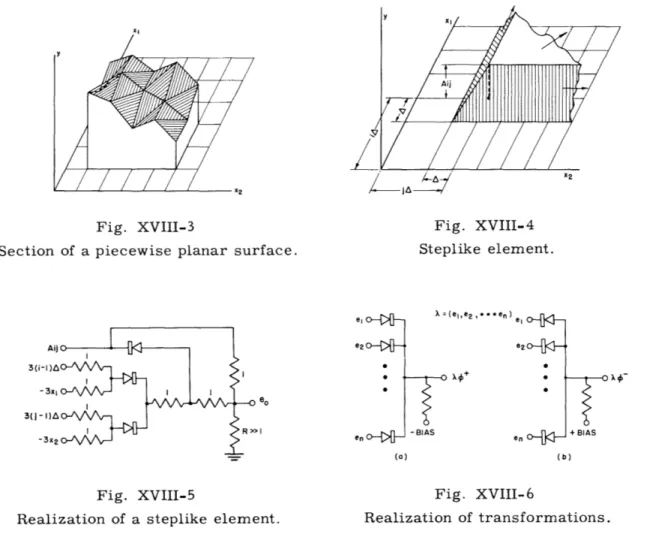
Figure XVIII-3 is an example of a portion of a surface approximated in this

manner.

The points of intersection are the given tabulated points.

(Note: In general,

an arbitrary surface must necessarily be approximated by triangular segments of

planes.)

This complex surface can be synthesized by the superposition of many simpler

sur-faces.

For example, the addition of "step" surfaces like the one shown in Fig. XVIII-4

produces a resultant surface similar to that shown in Fig. XVIII-3.

In order for the

resultant surface to coincide with the elements of the [aij] matrix, it must be constituted

of the summation of mn steplike elements (mn is the product of the dimensions of the

a matrix), each step being centered over a different tabulated point. The height, A..,

of a typical element centered over xl = iA, x

2 =

jA, must be

Aj

ij + a-l,

j-1

t-1, j

, -1

The circuit of Fig. XVIII-5 is one method of realizing a steplike element. An alternative

method of synthesizing a piecewise planar surface is the use of a summation of

square-pyramidal elements.

As one generalizes to functions of more than two variables, this procedure becomes

more involved.

For example, in dealing with functions of three variables, we find that

each region of analyticity must be a tetrahedronal element of volume bounded by four

planes rather than a triangular element of a plane bounded by three lines. In going to

still more dimensions, the bounding surfaces become hyperplanes, and visualization

becomes impossible.

b.

Algebra of piecewise linear functions

The synthesis techniques mentioned above are primarily based upon the

formu-lation of an algebraic notation that enables one to express the complete behavior

of a piecewise linear, or more generally, piecewise analytic, continuous function

as a single equation, rather than as a set of equations coupled with inequalities to

(5)

-86-Fig. XVIII-3

Fig. XVIII-4

Section of a piecewise planar surface. Steplike element.

* , (ele2 , * *e n ) e e2 en x

0-Fig. XVIII-5

Fig. XVIII-6

Realization of a steplike element. Realization of transformations.

show their regions of validity.

To accomplish this it is convenient to define two types of algebraic transformations:

1+

and c-.

Let X = (a, b, ... , n) where p is the greatest element in X and q is the least element in X. (X can be any set of elements of a well-ordered integral domain.) Then we define:

\

+ =p; O- = q.

By the use of suitable combinations of these transformations it is possible to elimi-nate the need of the conventional inequality relations that inevitably complicate the analysis of systems that are piecewise analytic in behavior.

These particular transformations are easily realizable electronically through the use of diodes, as illustrated in Fig. XVIII-6. (Note that the bias voltage must be greater in magnitude than the greatest of the elements of X.) Thus, once a piecewise linear function is represented in terms of these transformations, it is, at least in theory, a relatively simple matter to realize it electronically.

Investigation is in progress on the development of a suitable algebra for these sets

(6)

of elements and their transformations. The algebra is being developed along the lines of the algebra of vector spaces.

T. E. Stern

8. The Saturable Reactor in Analog Computers

In the effort to construct a driftless, high-gain dc amplifier, a type of modulated circuits have been developed (1). For modulation and demodulation, synchronous vibra-tors (choppers) or variable capacivibra-tors are used. The objection to these samplers is their dependence on a mechanical operation. For certain applications, a nonmechanical chopper has been developed whose operation relies on the resistance changes of a photo-sensitive crystal. In quest of other nonmnechanical choppers, the possibilities of the

saturable reactor were investigated, and some preliminary experiments have been performed on two types of saturable reactor circuits, with promising results.

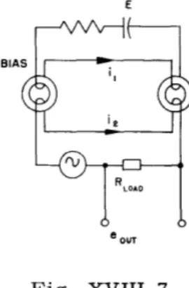
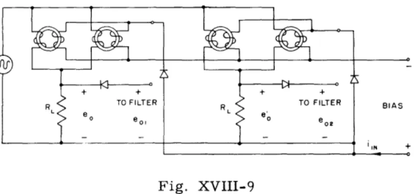
The first circuit consists of a series-connected, balanced saturable reactor (Fig. XVIII-7); the second, of a parallel-connected saturable reactor (Fig. XVIII-8). Both are driven from a square-wave voltage generator with very low internal impedance. With the former, a pulse-modulated signal having an amplitude proportional to the input bias is obtained at the output; with the latter, a pulse having a width proportional to the input is obtained. It should be noted that the sign-sensitive circuit that is required is obtained with a single core. However, for better waveshapes parallel-connected cores should be used; then the circuit is not sign-sensitive. To obtain the sign sensitivity two more parallel-connected cores are required, together with some additional circuitry, as shown in Fig. XVIII-9. The corresponding waveforms are shown in Fig. XVIII-10. The output is filtered (1), giving a positive or negative dc voltage proportional to the input offset voltage of the dc amplifier. The over-all gain (input-filtered output) should be of the order of 250, 000. Our circuit falls short of this number by a factor of about

15. Better design in the saturable reactor might give the required gain.

E

BIA

E.

Fig. XVIII-7 Fig. XVIII-8

Series-connected saturable reactors. Parallel-connected saturable reactors.

(7)

-88-Fig. XVIII-9

Circuit for the sign-sensitive magnetic chopper.

Ei SQUAREE- WAVE GENERATOR

eF-oU _U

C,,

I-

Fl

25 PERCENT PULSEWIDTH MODULATION, i,, >0 OUTPUT TO FILTER 25 PERCENT - [7 PULSEWIDTH MODULATION, I <0 e02 - _{OUTPUT TO FILTER}

Fig. XVIII-10

Waveforms for the circuit of Fig. XVIII-9.

Comparing the series and parallel circuits we realized that each has its own

advantages.

The first does not require sharp knee magnetization curves for the

cores, operates effectively on rather high input currents, but would require

com-plex circuitry for sign sensitivity.

The second relies upon very sharp knee

mag-netization curves, operates on small input currents, requires rather simple circuitry

for sign sensitivity, and can accommodate a predetermined maximum offset input

voltage, since for this maximum we have a 100 percent pulsewidth modulation.

A

further development of the second type may easily compete with the mechanical

chopper.

M. S. Macrakis

References

1. G. A. Korn and T. M. Korn, Electronic Analog Computers (McGraw-Hill

(8)

L RI

T

'T1

090 - 085--030 A0 O

₄

₀

- 065- 055-/00 900 -aoo 550 z 500 'O O60 20 380 360 20 310 tSro 280 .20 210 /80 7 533 133 06o 060 090 00 CJ

050

-C, I O

-

-90-W998 98 97 18 3o 879 o55o 5SO 3j0 30 1 80 260 / o0 ovo to /60 I 35 120 OYO 030

-:161

/19

Fig. XVIII-11

Nomogram for third-order Butterworth function with loss.

- --- -L __

"~---- ~~ --- ~ ~ - -I

(9)

B. APPLIED NETWORK THEORY

1. Complex Frequency Plane Synthesizer

A device has been constructed which has for its transfer function a pair of conjugate-complex poles in the conjugate-complex-frequency plane. The real and imaginary coordinates of these poles are independently and continuously adjustable by means of a system of ganged potentiometers. A switching system is provided so that the device can be used with the poles in either half-plane. The basic elements of the device are two integrators of the

"clamped" analog computer type.

Several of these elements can be cascaded for experimental synthesis of networks and the steady-state and transient responses are both available.

L. A. Irish

2. A Nomogram for a Butterworth Filter with Internal Loss

All of the modern methods of network synthesis yield lossless networks terminated in a single resistor. The addition of internal loss gives added flexibility in the design and is often desirable for itself. Scott's iterative method has been applied to the third-order Butterworth filter. A nomogram of the results is shown in Fig. XVIII-11.

J. P. Blake

3. An Approximate Method for Frequency Time Domain Transformation

In system or network analysis and synthesis, one is often faced with the problem of evaluating inverse L-transforms of the general type,

2 m

b0 + bs +b2s + .. +b s

F(s) = 2 mn ₍₁₎

a0 + als + a2s +... + ans

The classical approaches to this problem by integral equation or partial fraction expansion are usually lengthy and often very difficult to carry out for n > 4.

There exist several approximate semigraphical methods for this frequency time domain transform as described in references (1) and (2). The method (3) proposed here is entirely analytical and involves little or no graphical manipulation. Basically, one proceeds by replacing every s term in Eq. 1 by (1 - E-ST/T). Thus

m -ksT

-sT

-msT

m dk

sT

d +d + d..

Z

dk

F(s) -F* sT d + dE +. + k=0 ( (E

)

= -sT -2sT -nsT ( cO + C E + c E +... + C E c E -ksT k=0

(10)

(XVIII. ANALOG COMPUTER RESEARCH)

* -sT

do

0

d

-sT

-2ZsT

F (E

)=

+ l C j c

E

+ f0 f= E 2 C₀ =0/ 00 + fk -ksT + = -fkEksT f=0

This form is then easily transformed into time domain. The coefficient fk becomes the ordinate of f(t) at time kT.

The selection of the interval T in the approximation s - (1 - E-sT)/T is naturally important since it directly determines the accuracy. It is necessary to have some idea about the order of magnitude of the highest significant frequency component in the resul-tant time function before one can select T intelligently. If smax is the highest significant

frequency component, then Tmax should be

T

_max _{40 f}

1

_{6.5 s}

1 (3)

max max

corresponds to 5' of phase shift.

2 sT 2 3 -sT 3 3

However, the percentage error increases for s 2 (I-E- ) /T , s = (1- E ) /T 3 , and so on when the same T is used. Furthermore, all the error caused by approximating the different s terms in the function may add up as well as cancel out. Thus, as a first approximation,

1

Tmax n = order of the s transform (4)

max 6. 5 2 max

The advantage of this method lies chiefly in the fact that once the s-function is trans-formed into the so-called z-domain, all the sampled-data analysis techniques (4) already

developed are applicable. In many cases, analysis procedures are more easily handled or become intuitively obvious when they are in sampled-data form. For example, in

sampled-data language, one knows that the approximation s2

=

(1 -

E-

)/(T-sT) is much better than s2 = (1 - E-sT2 2. In the example shown in Fig. XVIII-12, f(t) is computed from F(s) using the above-mentioned method but with different approximation

2 *

sT

for s . The accuracy increases by three times in one case. Furthermore, once F (E

)

is obtained it is not necessary to determine f0, f, f2 . . . fk-l' before fk can finally be computed. One merely has to throw away successively the even or odd parts of

* -sT * -2sT * - 4sT

F (E ), F (E ), F

(E

), etc. For example, if it is necessary to determine f4

* -sT

sT

for F (E T ) one proceeds by throwing away first the odd part of F (E -S ) leaving

• 2sT . -2sT

F (E-2T) which is rational in E . This procedure can be repeated to obtain

F (E- 4 s T ) which contains only terms rational in

E-4sT

(11)

-92-m/4 _-4ks_T d4k E F*(E-sT) _F *(E-4sT k=4 (5) n C4/4 -4ksT I C4kE k=0

With one division, one obtains f4'

In short it is interesting to note how the various sampled-data techniques fit into this method of approach. Further investigation into the practical application of this method to system design is under way.

Y. C. Ho

References

1. G. S. Brown and D. P. Campbell, Principles of Servomechanisms (John Wiley and Sons, Inc., New York, 1948) Chapter 11.

2. E. A. Guillemin, Technical Report No. 268, Research Laboratory of Electronics, M.I.T., Sept. 2, 1953.

3. A paper of similar nature, entitled "A mathematical technique for the analysis of linear systems," was published during this period of research by J. R. Ragazzini and A. R. Bergen of Columbia University.

4. For detailed descriptions of these techniques see Whirlwind Report R-222 by W. K. Linvill and R. Sittler and other papers by W. K. Linvill.

0.8- f(t)= 1.07 -0.5t COS(.323t-20.7o)

S+I

F(s) =F) S2+S+2

0.6 \ (I- -$T)

2 0.6- _{FUNCTION COMPUTED USING}

S = T2

WITH T= 1/30

--- FUNCTION COMPUTED USING S

2

(I--T

0.4 t WITH T=1/1O

To-T 000 CHECK POINTS 0.2 -1/3 2/3 I 4/3 5/3 2 t

-0.2--0.4 Fig. XVIII-12 Plot of computed f(t).

(12)

4. Duality of Ideal Transformers

In the Quarterly Progress Report of January 15, 1954, the analysis of ideal trans-formers was based on a pair-terminal view; that is, using input and output voltages and currents with no attention to the specific geometric configuration of the transformer.

The ideal transformer was defined as a specified ratio of a number of voltages some-where in the system. Windings were used only as a means of graphical presentation.

In practice, the best that one can do is to approximate this concept with actual windings; and the topological aspects of this physical system play an important role in the over-all analysis. The problem of duality of ideal transformers is considered on a purely topological basis.

Duality of two electrical networks is here defined by the relations: V , I; I - V; where the symbol " - " is used for "dual of."

On examining the elementary circuit of a two-winding transformer, one sees instantly that the quantities flux

4

and mmf F are directly related to the topological nature of the system. They are related to the voltages and currents as follows:

F = NI X = NP Edt (1)

F - I - QE (2)

where the symbol -- indicates "topologically equal." The letter

Q

indicates an operation with no topological consequences. Equations 2 have led a number of writers to consider F and as excitation and response quantities, respectively, or vice versa. The main point is that these quantities are interrelated through the electrical and topological properties of the "magnetic" medium.

To represent the topological properties of a transformer one needs to make a "ring" diagram where the current and flux paths are designated with solid and broken rings, respectively. This type of diagram preserves only the "linked" topological dependence of the physical quantities F and

P.

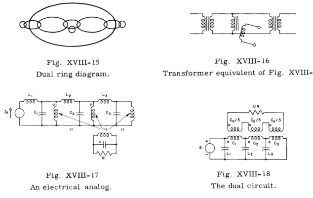
The scheme is best illustrated by the examples shown in Figs. XVIII-13 and XVIII-14. In Fig. XVIII-14 the parallel lines in the

I

-N

-Fig. XVIII-13 Fig. XVIII-14

A transformer.

A ring diagram.

(13)

-94-I

il

Fig. XVIII- 15

Fig. XVIII- 16

Dual ring diagram.

Transformer equivalent of Fig. XVIII-15.

L L2 L3

sI/R

E

R