Applications of twitter emotion detection for stock market prediction

Applications of Twitter Emotion Detection for Stock

Market Prediction

by

Clare H. Liu

S.B., Massachusetts Institute of Technology (2016)

Submitted to the Department of Electrical Engineering and Computer

Science

in partial fulfillment of the requirements for the degree of

Master of Engineering in Computer Science and Engineering

at the

MASSACHUSETTS INSTITUTE OF TECHNOLOGY

June 2017

c

○

Massachusetts Institute of Technology 2017. All rights reserved.

Author . . . .

Department of Electrical Engineering and Computer Science

May 18, 2017

Certified by. . . .

Andrew W. Lo

Charles E. and Susan T. Harris Professor

Thesis Supervisor

Accepted by . . . .

Christopher J. Terman

Chairman, Masters of Engineering Thesis Committee

Applications of Twitter Emotion Detection for Stock Market

Prediction

by

Clare H. Liu

Submitted to the Department of Electrical Engineering and Computer Science on May 18, 2017, in partial fulfillment of the

requirements for the degree of

Master of Engineering in Computer Science and Engineering

Abstract

Currently, most applications of sentiment analysis focus on detecting sentiment polar-ity, which is whether a piece of text can be classified as positive or negative. However, it can sometimes be important to be able to distinguish between distinct emotions as opposed to just the polarity. In this thesis, we use a supervised learning approach to develop an emotion classifier for the six Ekman emotions: joy, fear, sadness, disgust, surprise, and anger. Then we apply our emotion classifier to tweets from the 2016 presidential election and financial tweets labeled with Twitter cashtags and evaluate the effectiveness of using finer-grained emotion categorization to predict future stock market performance.

Thesis Supervisor: Andrew W. Lo

Acknowledgments

First of all, I would like to express my gratitude to my thesis supervisor, Professor Andrew Lo, for giving me the opportunity to explore a new field, and for his insightful ideas and feedback. I would also like to thank Allie, Jayna, and Crystal for providing me with important resources and for their scheduling help.

I especially want to thank Shomesh Chaudhuri for giving me crash courses on finance and providing invaluable suggestions and guidance over the past two years.

Finally, I wish to thank my parents for their unconditional support and encour-agement.

Contents

1 Introduction 13

1.1 Thesis Organization . . . 14

2 Literature Review 17 2.1 Emotion Classification . . . 17

2.2 Relationship Between Twitter Sentiment and Stock Market Performance 19 2.3 Predicting Presidential Elections . . . 21

3 Creating an Emotion Classifier 23 3.1 Multiclass Classification Algorithms . . . 23

3.1.1 One-vs-rest . . . 24 3.1.2 One-vs-one . . . 24 3.1.3 Logistic Regression . . . 24 3.1.4 Random Forests . . . 25 3.2 Datasets . . . 26 3.3 Baselines . . . 26 3.4 Methodology . . . 27 3.4.1 Feature Selection . . . 27 3.4.2 Data Preparation . . . 28 3.4.3 Implementation Details . . . 28 3.5 Evaluation Metrics . . . 29 3.6 Results . . . 31 3.7 Discussion . . . 32

4 Emotion Analysis of Presidential Election Tweets 35

4.1 Datasets . . . 35

4.1.1 Data Preparation . . . 36

4.2 Emotion Distributions on Election Day . . . 36

4.2.1 Election Day Key Events . . . 37

4.2.2 Comparison with Polarity-Based Sentiment Analysis . . . 37

4.2.3 Using Volume to Identify Events . . . 40

4.3 Can Presidential Debates Predict Market Returns? . . . 42

4.3.1 Summary of Candidate Policies . . . 42

4.3.2 S&P 500 Returns after Election Day . . . 43

4.3.3 Who won the Presidential Debates? . . . 44

4.3.4 S&P 500 Reactions to Presidential Debates . . . 46

4.4 Discussion . . . 48

5 Emotion Analysis of Financial Tweets 51 5.1 Datasets . . . 51

5.2 Correlation Between Emotions and Stock Prices . . . 52

5.3 Using Volume to Identify Events . . . 55

5.4 Sentiment-Based Trading Strategy . . . 57

5.4.1 Preliminary Results . . . 58

5.4.2 Reevaluation of Emotion Classifier Performance . . . 61

5.5 Keyword-Based Trading Strategy . . . 65

5.5.1 Evaluation of Trading Strategy Performance . . . 66

5.6 Discussion . . . 68 6 Conclusions and Future Work 69

List of Figures

4-1 Average Sentiment during the 2016 Presidential Election . . . 37

4-2 2016 Election Day Emotion Distributions . . . 39

4-3 First Presidential Debate . . . 41

4-4 Emotion Distributions during the First Presidential Debate . . . 44

5-1 Twitter Volume Plots for Microsoft and Facebook . . . 57

5-2 Preliminary Trading Strategy Performance for Microsoft, Facebook, and Yahoo . . . 60

5-4 Microsoft sentiment using keywords during earnings announcement on April 21 . . . 65

List of Tables

3.1 Examples of Labeled Tweets . . . 26

3.2 Tweet Processing Example . . . 28

3.3 Model Comparison . . . 31

3.4 Logistic Regression Accuracy Metrics . . . 32

3.5 Classification Examples . . . 33

3.6 Examples of Classification Errors . . . 34

4.1 S&P 500 Sectors before and after Election Day . . . 43

4.2 Clinton: Change in joy tweets before and after debates . . . 45

4.3 Trump: Change in joy tweets before and after debates . . . 45

4.4 Morning Consult Poll Results . . . 46

4.5 S&P 500 Industries Before and After First Presidential Debate . . . 46

4.6 S&P 500 Industries Before and After Second Presidential Debate . . 47

4.7 S&P 500 Industries before and after Third Presidential Debate . . . 48

5.1 Correlation between average emotion percentages and next-day stock returns . . . 53

5.2 Correlation between average emotion percentages and same-day stock returns . . . 54

5.3 Noise in $AAPL Tweets . . . 55

5.4 Microsoft Earnings Announcement Classification Examples . . . 62

5.5 Yahoo Earnings Announcement Classification Errors . . . 63

5.6 Trading Strategy Comparison . . . 67

Chapter 1

Introduction

Over the past decade, the rise of social media has enabled millions of people to share their opinions and react to current events in real time. As of June 2016, Twitter has over 300 monthly active users and over 500 million tweets are posted per day [53]. Ever since the official Twitter API was introduced in 2006, users and researchers have been applying sentiment analysis algorithms on this massive data source to gauge public opinion towards emerging events. Automatic sentiment analysis algorithms have been used in a variety of applications, including evaluating customer satisfaction, fraud detection, and predicting future events, such as the results of a presidential election. Currently, most publicly available sentiment analysis libraries focus on detecting sentiment polarity, which is whether a piece of text expresses a positive, negative, or neutral sentiment. However, due to the wide range of possible human emotions, there are some limitations to using this coarse-grained approach for some applications. For instance, the producers of a horror movie may wish to use sentiment analysis to summarize understand their audience’s opinion of the movie. Boredom and fear could both be classified as negative emotions, but the producers would be happy if their viewers expressed fear, while they would probably modify their approach for future movies if the viewers were bored.

In this thesis, we will evaluate the merits and limitations of using a finer-grained emotion classification scheme compared to the more common sentiment polarity ap-proach. We will also evaluate the possibility of predicting future stock returns based

on emotion distributions of tweets from two contrasting domains: presidential elec-tions and financial tweets mentioning NASDAQ-100 companies. The election of a new president has wide implications on the future of United States and international economies, which usually results in stock market volatility. Company stock prices have also been shown to be affected by market sentiment, especially following impor-tant events such as earnings announcements and acquisitions.

Since presidential elections and volatility in the stock market often evoke strong emotions in people, using a finer-grained emotion analysis approach could reveal more interesting insights about the public’s perception of candidates and publicly traded companies, potentially leading to more accurate and profitable stock market predictions.

1.1 Thesis Organization

The remainder of this thesis is organized as follows:

∙ Chapter 2 contains a literature review of past work in automatic emotion de-tection and in using Twitter to predict future stock market performance and the results of presidential elections.

∙ Chapter 3 then details the construction of and evaluates the performance of an emotion classifier for the six basic Ekman emotions.

∙ In chapter 4, we analyze tweets from the 2016 presidential election to determine whether emotion classification can be used to identify differences in public opin-ion towards the two presidential candidates. Then we investigate the correlatopin-ion between the policies of presidential debate winners and the market performance of related industries on the following day.

∙ In chapter 5, we will evaluate the correlation between emotion distributions of tweets tagged with cashtags of the NASDAQ-100 companies and future stock returns for these companies. We then look at trends in Twitter volume and

sentiment for different tickers to identify significant events and predict outcomes on future returns. Finally, we will propose a simple trading strategy based on sentiment expressed in earnings announcement tweets.

∙ Finally, chapter 6 will summarize our major findings and suggest possible av-enues for future research.

Chapter 2

Literature Review

This chapter discusses approaches to automatic emotion classification and related work in using social media for stock market prediction.

2.1 Emotion Classification

In 1992, psychologist Paul Ekman argued that there are six basic emotions: anger, fear, sadness, joy, disgust, and surprise. These emotions share nine characteristics with a biological basis, including distinctive universal signals, presence in other pri-mates, and quick onset. He also argued that all other emotional states can be grouped into one of these basic emotions or classified as moods, emotional traits, or emotional attitudes instead [11].

Much of the recent research on finer-grained emotion detection has been focused on these six basic Ekman emotions. In 2007, SemanticEvaluation, an ongoing series of evaluations of computational semantic analysis systems, presented a task where the objective was to "annotate text for emotions (e.g. joy, fear, surprise) and/or for polarity orientation (positive/negative)" [51]. Participants were provided with a development corpus of 250 news headlines annotated with one of the six Ekman emotions and a test corpus of 1000 news headlines. Many future studies on emotion detection used this corpus to develop classifiers and larger corpora annotated with emotions.

Roberts and Harabagiu et al. developed EmpaTweet, a corpus of tweets anno-tated with the six Ekman emotions plus "love" using a semi-automated process [42]. Roberts first used a supervised learning approach to first automatically annotate unlabeled tweets with one or more emotional categories. Then human annotators were asked to verify the predominant emotion for ambiguous tweets. Mohammad et al. also created the Twitter Emotion Corpus (TEC) by collecting tweets containing hashtags of the six Ekman emotions, such as #joy and #sadness [30].

Two major approaches to automatic emotion classification include supervised learning methods and affect lexicon-based approaches [31]. Supervised learning ap-proaches generally analyze labeled training examples to generate a prediction function that can be applied to unseen data. Many supervised learning algorithms use 𝑛-gram features to learn which words or phrases in the training data are associated with each emotion.

An affect lexicon is a list of words and the emotions or sentiment that they are associated with. For example, the word "abandoned" is associated with fear and sadness, while "amuse" is associated with joy. Lexicon-based approaches usually look up the emotion associated with each word in a piece of text, if any, and label the text with the predominant emotion that was present. One example of an affect lexicon is Mohammad and Turney’s NRC Word-Emotion Association Lexicon (EmoLex), which they generated using crowdsourcing from Amazon Mechanical Turk [29] [32].

Lexicon-based approaches usually perform worse than supervised learning ap-proaches because they don’t consider the context or sentence structure, which can greatly affect the meaning of a piece of text. However, lexicon-based approaches are much faster and more memory efficient than supervised learning methods, which usually use tens of thousands of features to generate models. Supervised learning approaches also may not generalize as well to other domains that do not share many 𝑛-gram features with the training set.

Mohammad then investigated whether combining affect lexicons and 𝑛-gram fea-tures in a supervised learning algorithm could improve the accuracy of a classifier [31]. He found that using a combination of both types of features outperformed using

𝑛-grams alone and affect lexicon features alone for test sets containing samples from the same domain (newspaper headlines) and a different domain (blog posts). Thus, we decided to replicate Mohammad’s approach of using both 𝑛-grams and word lexicon features in our classifier.

Next, we will discuss previous studies on the effectiveness of using both polarity-based sentiment analysis and emotion classification to predict future stock market movements.

2.2 Relationship Between Twitter Sentiment and Stock

Market Performance

Several groups have studied the correlation between sentiment polarity and the per-formance of various stock market indicators. Many studies found that sentiment polarity was not useful for predicting future stock returns, but that other factors such as volume were. Ranco et al. measured the correlation between Twitter vol-ume and sentiment of Dow Jones constituents and the Dow Jones Industrial Average (DJIA). They found that sentiment polarity was not correlated with future stock re-turns, but that tweet volume was predictive of abnormal returns for about one third of the 30 Dow Jones companies. [40]. Hentschel et al. then studied the properties of Twitter cashtags for NASDAQ and NYSE stocks. They also found that tweet volume and market performance are sometimes related, but not always [19]. The correlation between tweet volume and future returns suggests that increases in tweet volume can be indicators of important events that can impact the market.

Azar and Lo focused specifically on tweets mentioning the Federal Open Market Committee from 2009 - 2014 and calculated the sentiment polarity for these tweets, weighting the polarity values by each Twitter user’s number of followers. They found that the effect of sentiment polarity on returns was negligible except on the eight days that the FOMC meets, where increases in sentiment polarity are positively correlated with returns [3]. Furthermore, they were able to develop a sentiment-based trading

strategy that significantly outperformed benchmarks, even when only using eight days of data. Therefore, sentiment polarity seems to have the most predictive value when applied to significant market events.

Other studies focused on identifying emotions or moods expressed in tweets and other forms of social media. Bollen et al. measured the mood of tweets in six di-mensions (Calm, Alert, Sure, Vital, Kind, and Happy) in addition to their polarity (positive/negative). Like Ranco, they found that just the polarity of tweets was not correlated with future stock returns, but that the calmness dimension could be used to predict movements in the Dow Jones Industrial Average [6]. Mittal and Goel also found that calmness and happiness had a strong positive correlation with the DJIA. They were also able to accurately predict future DJIA closing prices using a neu-tral network algorithm and develop an improved portfolio management strategy that makes buy and sell decisions based on whether predicted future stock prices are above or below the mean values [28].

Gilbert and Karahalios used a supervised learning approach to create the "Anxiety Index", a metric of anxiety, fear, and worry expressed in blog posts published on LiveJournal. They found that increases in anxiety, worry, and fear across all of LiveJournal predicted downward pressure on the S&P 500 index, even when including blogs not related to finance [16]. Zhang et al. used a simpler approach to categorize tweets into the six Ekman emotions by counting words associated each emotion. Interestingly, they found that outbursts of both positive and negative emotions on Twitter had a negative correlation with the Dow Jones, S&P 500, and NASDAQ indices [56].

These results support our hypothesis that categorizing tweets into finer-grained emotions can be more useful than classifying tweets as just positive or negative for stock market prediction.

2.3 Predicting Presidential Elections

Twitter sentiment analysis has also been used to predict the results of presidential elections. Jahanbakhsh and Moon performed a variety of analysis techniques, such as studying frequency distributions, sentiment analysis, and topic modeling to identify topics discussed in tweets during the 2012 presidential election [22]. They were able to determine that Obama was leading during the election from only analyzing Twitter data, which demonstrates the potential predictive power of Twitter for elections.

Shi et al. investigated public opinion on Twitter during the 2012 republican pri-mary election. They tested the correlation between various Twitter factors, including the Twitter volume for each candidate, the geolocation of Twitter users, and whether the Twitter account is a promotional account, and official poll results from the Real-clearpolitics website. Their algorithm was able to accurately predict public opinion trends for Mitt Romney and Newt Gingrich, two out of the four candidates. Again, they found that their results when combining Twitter sentiment with volume were very similar to using volume alone [48].

In addition, presidential election results have also been shown to be tied to future stock returns. Prechter et al. found that social mood reflected by the stock market was more predictive of the success of an incumbent president’s reelection bid than traditional macroeconomic factors, such as the Gross Domestic Product, inflation rate, and unemployment rate [39].

Oehler et al. analyzed stock market returns following presidential elections from 1976 to 2008 and found that the election of almost all recent presidents caused ab-normal returns in many sectors and industries, but that the stock returns eventually stabilized with time. They also discovered that these effects were more correlated with the specific policies of individual presidents rather than the general ideology of the president’s political party. They hypothesized that this effect is caused by initial uncertainty about the president-elect’s new policies [35].

These results suggest that we can use a combination of Twitter volume and sen-timent to gauge public opinion towards presidential candidates, which can in turn be

Chapter 3

Creating an Emotion Classifier

Many corpora and libraries are publicly available for polarity-based sentiment anal-ysis. However, finer-grained emotion categorization has not been studied as much, so we will develop our own emotion classifier to label unseen tweets with one of the six Ekman emotions in this chapter. This chapter will first summarize several ap-proaches to multiclass classification, and then describe the implementation of our emotion classifier and evaluate its performance.

3.1 Multiclass Classification Algorithms

Many machine learning classification algorithms are designed to classify input ex-amples into two groups, such as positive and negative. These binary classification algorithms generally work by generating features for each training example and then calculating a decision boundary between the two classes.

However, since we want to classify each tweet as one of the six basic Ekman emo-tions, we must use a multiclass classification approach. Multiclass classification solves the problem of assigning labels to a set of input examples, where there are more than two classes [1] [2]. Most multiclass classification approaches are based on binary clas-sification methods. The one-vs-rest and one-vs-one strategies work by reducing the problem into multiple binary classification tasks. Other binary classification algo-rithms, such as logistic regression and random forests, can naturally be extended to

multiclass problems. All of these approaches are summarized below.

3.1.1 One-vs-rest

The one-vs-rest approach trains a single binary classifier per class, where samples from each class are treated as positive samples and all other samples are negative samples. Each classifier produces a real-valued confidence score instead of just a class label. Then we can apply each classifier to each unseen sample and choose the label that corresponds to the classifier with the highest confidence score. The following equation describes how a label is chosen for each sample.

ˆ

𝑦 = arg max

𝑘∈1...𝐾

𝑓𝑘(𝑥) (3.1)

If we have 𝐾 classes, for each unseen sample 𝑥, we apply each of the 𝐾 classifiers to the sample. 𝑓𝑘(𝑥) represents the confidence score obtained by applying classifier

𝑘 to sample 𝑥. Then we choose the label ˆ𝑦 to be the class 𝑘, where 𝑓𝑘 produces the

highest confidence score [1] [2].

3.1.2 One-vs-one

The one-vs-one method trains 𝐾(𝐾−1)

2 binary classifiers between each pair of the 𝐾

total classes. Each of these classifiers is applied to all unseen samples and a voting scheme is applied, where each binary classifier votes for the class that produced the higher confidence score. The class with the highest number of votes is ultimately predicted for each sample [1] [2].

3.1.3 Logistic Regression

Linear regression is another classification algorithm that predicts real-valued outputs based on a linear function of the input examples. The basic linear prediction function is given in equation 3.2, where 𝑥 is a vector containing the features of the training samples, 𝑦 is a vector of predicted labels, and 𝜃 refers to the parameters of the model

[34].

𝑦 = ℎ𝜃(𝑥) =

∑︁

𝑖

𝜃𝑖𝑥𝑖 = 𝜃𝑇𝑥 (3.2)

However, the linear regression model does not work well for classifying examples into a few discrete classes. Thus, the logistic regression classifier uses the sigmoid function in equation 3.3 to map the output of the linear prediction function into the range [0,1]. Thus, ℎ𝜃(𝑥) represents the probability that a 𝑥 is a positive example.

Similarly, 1 − ℎ𝜃(𝑥)represents the probability that 𝑥 is a negative example [34].

𝑃 (𝑦 = 1|𝑥) = ℎ𝜃(𝑥) =

1

1 + exp (−𝜃𝑇_𝑥) (3.3)

For multiclass classification with 𝐾 classes, we can use multinomial logistic re-gression, which runs 𝐾 − 1 independent binary logistic regression models. One class is chosen as a pivot value and the other 𝐾 − 1 classes are compared against this probability value. Finally, the class with the highest probability score is predicted, similarly to the one-vs-rest algorithm described above [27].

3.1.4 Random Forests

The random forest classification algorithm is an ensemble learning method based on decision trees. Decision trees are made up of decision nodes and leaves, which each represent a possible class. At each decision node, we examine a single variable, and we choose another node based on the result of a comparison function using the sample’s features as inputs. The final leaf we choose is outputted as the predicted label [43].

The random forest algorithm constructs many decision trees and outputs the class that was the most frequently predicted by each of the individual decision trees. Com-bining the results of multiple decision trees helps to correct for a single decision tree’s tendency to overfit to its training set [20].

3.2 Datasets

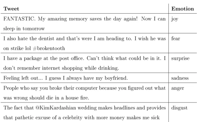
We use Mohammad’s Twitter Emotion Corpus (TEC) as training data for our clas-sifier. This corpus contains over 21,000 tweets annotated with one of the six Ekman emotions [30]. We also used Mohammad and Turney’s NRC Word-Emotion Associ-ation Lexicon (EmoLex) to identify words that are associated with each of the six Ekman emotions. EmoLex is an affect lexicon that contains over 14,000 English words and a list of the Ekman emotions each word is associated with. Table 3.1 shows examples of tweets in the TEC that are labeled with each of the six Ekman emotions.

Table 3.1: Examples of Labeled Tweets

Tweet Emotion

FANTASTIC. My amazing memory saves the day again! Now I can sleep in tomorrow

joy

I also hate the dentist and that’s were I am heading to. I wish he was on strike lol #brokentooth

fear

I have a package at the post office. Can’t think what could be in it. I don’t remember internet shopping while drinking.

surprise

Feeling left out... I guess I always have my boyfriend. sadness People who say you broke their computer because you figured out what

was wrong should die in a house fire.

anger

The fact that @KimKardashian wedding makes headlines and provides that pathetic excuse of a celebrity with more money makes me sick

disgust

3.3 Baselines

We implemented two simple baseline approaches to allow us to better evaluate the performance of our emotion classifier. The first baseline we tested was random guess-ing for each emotion, where each tweet is assigned a random number between 1 and 6, and each number corresponds to one of the six Ekman emotions. This approach

had an average 10-fold cross validation score of 0.1667 over 20 trials.

In addition, we implemented an affect lexicon approach by counting words corre-sponding to each of the six emotions in and labeling tweets the emotion associated with the greatest number of words. This approach had a 10-fold cross validation score of 0.275, which slightly outperforms the random guessing approach. However, even though every tweet in the training set was labeled with one of the six Ekman emotions, 50.31 % of the tweets in the training set did not contain any emotion words. For example, the tweet "One more week and I’m officially done with my first semester of college.", clearly expresses joy, but since none of the joy words are contained in this tweet, this tweet would be classified as neutral.

The poor performance of our baseline approaches indicates that a supervised learn-ing approach is necessary in order to develop a classifier with acceptable accuracy scores.

3.4 Methodology

This section describes the implementation of our classifier using a supervised learning approach, including feature selection and preprocessing of the training corpus.

3.4.1 Feature Selection

Since tweets are limited to 140 characters, the main idea of each tweet can usually be captured in just a few words. Therefore, we chose to use simple features, such as the presence or absence of unigrams and bigrams that appeared more than once in the training corpus. Bigrams were included to account for negation and basic sentence patterns that can affect the meaning of a tweet. For example, the phrase "not happy" conveys the opposite emotion as "happy", even though both phrases contain exactly one word that is associated with the joy emotion. We also chose to include features corresponding to the number of words associated with each of the Ekman emotions, as described in the second baseline above, since Mohammad found that including affect lexicon features improved classifier performance across different domains [31].

3.4.2 Data Preparation

All words in the NRC Lexicon and all unigrams and bigrams in all tweets were converted to lowercase and stemmed with NLTK’s Snowball Stemmer. This is to ensure that two English words with the same base word, but different tenses or forms would be treated as the same word. Stemmers work by removing suffixes to extract the base word [37]. For example, the words "organized" and "organizing" would both be converted to "organize".

Punctuation marks are also treated as separate words, because some punctuation marks can be used to emphasize an emotion. For instance, exclamation points are often used when expressing joy and question marks are used when expressing surprise. All other special characters are removed from tweets. Table 3.2 shows an example of a tweet before and after it has been processed.

Original Tweet "I will NOT go to he’d until I have my eyebrows threaded and my Mani/ Pedi... As a matter of fact I will be sleeping on the chair!!"

Processed Tweet "i will not go to he’d until i have my eyebrow thread and my mani pedi . . . as a matter of fact i will be sleep on the chair ! !"

Table 3.2: Tweet Processing Example

3.4.3 Implementation Details

Features are stored in the matrix 𝑋, where 𝑋 is an 𝑚 × 𝑛 matrix, where each row represents a sample and each column represents a feature. 𝑋[𝑖, 𝑗] corresponds to the value of feature 𝑗 for sample 𝑖. The matrix 𝑦 is an 𝑚 × 1 matrix that stores labels, so 𝑦[𝑖] corresponds to the label for sample 𝑖.

To populate the feature vectors, all unique unigrams and bigrams in the training corpus were assigned an index 𝑗 between 0 and 𝑚 − 1. At the prediction stage, all tweets are stemmed and separated into unigrams and bigrams. If 𝑛-gram 𝑗 is present

in tweet 𝑖, 𝑋[𝑖, 𝑗] is set to 1 to indicate the presence of a particular 𝑛-gram. Because the training set contains over 35,000 unique stemmed unigrams and bigrams, and the vast majority of the unigrams and bigrams will not appear in a particular tweet, we use sparse matrices for space efficiency. Six additional features were added to represent the counts of words from each emotion category from EmoLex.

Since the training set did not contain any examples of neutral tweets that ex-pressed no emotion, tweets expressing no emotion will be erroneously classified. Therefore, we also used Pattern to calculate the sentiment polarity of each tweet. Pattern is a web mining Python module that includes sentiment analysis and natural language processing tools. Pattern utilizes SentiWordNet, a corpus of English words annotated with a positivity, negativity, and objectivity scores for each word, to cal-culate polarity scores. Pattern then groups each tweet into varying sizes of 𝑛-grams and averages the positivity, negativity, and objectivity scores for each group of words to calculate a final polarity and subjectivity score. Adjectives and adverbs can also amplify or negate the polarity score of a tweet [10].

Pattern’s sentiment module reports a sentiment polarity ranging between -1 and 1, and a subjectivity score for each tweet ranging from 0 to 1 [10]. A polarity score of -1 means that the tweet is totally negative, 0 represents a neutral tweet, and 1 represents a totally positive tweet. We reclassified any tweets with a sentiment polarity score of 0.0 as neutral.

We then tested various multiclass classification algorithms implemented in scikit-learn modules to determine the algorithm that would produce the best accuracy for our training set. The algorithms we tested included support vector machines using the one-vs-rest and one-vs-all strategies, logistic regression, and random forests [33].

3.5 Evaluation Metrics

Since no test set was provided, we used scikit-learn’s built-in cross_val_predict function to evaluate the performance of our classifiers. cross_val_predict works by splitting the training set into 𝑛 equal-sized groups. For each group 𝑖, the other 𝑛 − 1

groups are used as training data and predictions are made for group 𝑖, treating group 𝑖as the test set. This process is repeated for all of the 𝑛 groups until every sample has been included in the test set exactly once. The cross_val_predict function returns the predicted labels for each element when that element was part of the test set [9].

We used the output from cross_val_predict to compute precision, recall, and F1 scores to evaluate each of the four models we tested. For a binary classification problem, precision represents the percentage of samples predicted as positive that are actually positive. Recall represents the percentage of actual positive samples that were predicted as positive by the classifier. The F1 score is a harmonic mean of the precision and recall and is often the main metric used to evaluate a classifier’s performance, since it is possible to design naive classifiers with artificially high precision or recall scores. For example, a classifier that predicts every sample as positive would have a 100 percent recall score. The equations for calculating precision, recall, and F1 scores are listed in equations 3.4 to 3.6. 𝑡𝑝, 𝑓𝑝, and 𝑓𝑛 represent true positives (sample is positive and was predicted as positive), false positives (sample is not positive, but was predicted as positive), and false negatives (sample is positive, but was predicted as negative) respectively. 𝑃 𝑟𝑒𝑐𝑖𝑠𝑖𝑜𝑛 = 𝑡𝑝 𝑡𝑝 + 𝑓 𝑝 (3.4) 𝑅𝑒𝑐𝑎𝑙𝑙 = 𝑡𝑝 𝑡𝑝 + 𝑓 𝑛 (3.5) 𝐹 1 = 2 · 𝑝𝑟𝑒𝑐𝑖𝑠𝑖𝑜𝑛 · 𝑟𝑒𝑐𝑎𝑙𝑙 𝑝𝑟𝑒𝑐𝑖𝑠𝑖𝑜𝑛 + 𝑟𝑒𝑐𝑎𝑙𝑙 (3.6) We can extend these evaluation metric calculations to multiclass problems by calculating each metric individually for all classes and then calculating the weighted average. For the "joy" class, all samples that are labeled with "joy" are counted as positive, while all other samples are counted as negative, and likewise for all other classes. Then the binary classification formulas for precision, recall, and F1 scores can be directly applied.

3.6 Results

Table 3.3 shows the precision, recall, and F1 results for each of the four models we tested.

Table 3.3: Model Comparison

emotion Precision Recall F1 One-vs-rest (SVM) 0.590 0.597 0.592

One-vs-all (SVM) 0.577 0.585 0.579 Logistic Regression 0.606 0.614 0.605 Random Forest 0.541 0.524 0.478

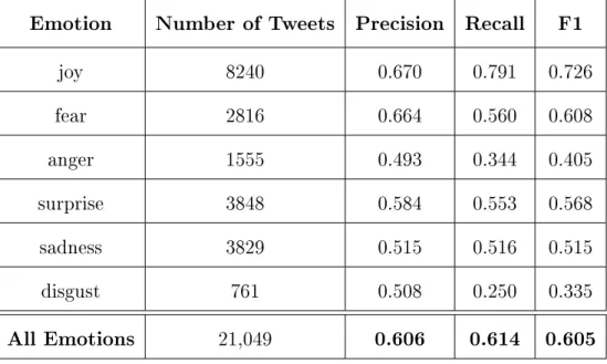
All four supervised learning machine learning models significantly outperformed our baselines of random guessing and only using an affect lexicon. The logistic re-gression model performed the best for all three evaluation metrics, so we will use this model for all classification problems throughout this thesis. Table 3.4 shows the precision, recall, and F1 scores for each emotion class for our logistic regression model.

Table 3.4: Logistic Regression Accuracy Metrics

Emotion Number of Tweets Precision Recall F1 joy 8240 0.670 0.791 0.726 fear 2816 0.664 0.560 0.608 anger 1555 0.493 0.344 0.405 surprise 3848 0.584 0.553 0.568 sadness 3829 0.515 0.516 0.515 disgust 761 0.508 0.250 0.335 All Emotions 21,049 0.606 0.614 0.605

The joy emotion had the highest F1 score and the disgust emotion had the lowest F1 score. This observation can be explained by the fact that joy is the only positive Ekman emotion, while it is more difficult to distinguish between the other Ekman emotions. In addition, joy was also the most common emotion in the training set, while disgust was the least common.Therefore, obtaining more training examples could help improve the classifier’s accuracy.

3.7 Discussion

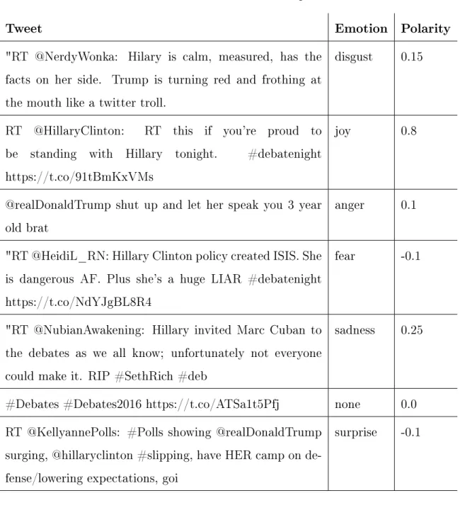
We looked at a sample of tweets from the 2016 presidential debates to subjectively evaluate the classifier’s performance on unseen data. In general, the classifier seems to work well since Twitter’s character limit usually prevents users from expressing multiple conflicting emotions in a single tweet. Table 3.5 shows some example tweets where the classifier predicted the correct emotion. Many of these tweets contain words or phrases that are strongly associated with an emotion, such as "dangerous" for fear, and "shut up" for the anger emotion.

Table 3.5: Classification Examples

Tweet Emotion Polarity

"RT @NerdyWonka: Hilary is calm, measured, has the facts on her side. Trump is turning red and frothing at the mouth like a twitter troll.

disgust 0.15

RT @HillaryClinton: RT this if you’re proud to be standing with Hillary tonight. #debatenight https://t.co/91tBmKxVMs

joy 0.8

@realDonaldTrump shut up and let her speak you 3 year old brat

anger 0.1

"RT @HeidiL_RN: Hillary Clinton policy created ISIS. She is dangerous AF. Plus she’s a huge LIAR #debatenight https://t.co/NdYJgBL8R4

fear -0.1

"RT @NubianAwakening: Hillary invited Marc Cuban to the debates as we all know; unfortunately not everyone could make it. RIP #SethRich #deb

sadness 0.25

#Debates #Debates2016 https://t.co/ATSa1t5Pfj none 0.0 RT @KellyannePolls: #Polls showing @realDonaldTrump

surging, @hillaryclinton #slipping, have HER camp on de-fense/lowering expectations, goi

surprise -0.1

However, our classifier does not perform as well on certain types of tweets. Table 3.6 shows some examples of tweets that have been misclassified. Relying on Pattern to identify neutral tweets introduces more errors because sentiment polarity algorithms are not completely accurate either. The first tweet clearly expresses joy and the second tweet expresses disgust, but our classifier predicted them as being neutral because the Pattern sentiment analysis algorithm assigned them polarities of 0.0.

Table 3.6: Examples of Classification Errors

Tweet Emotion Polarity

@HillaryClinton HILLARY HAS GOT TRUMP SOOO OUTCLASSED!!!!

none 0.0

RT @realDonaldTrump: Hillary is the most corrupt per-son to ever run for the presidency of the United States. #DrainTheSwamp https://t.co/xA

none 0.0

Three key questions for Trump and Clinton ahead of the first debate #Debates2016 https://t.co/YiCs6lwTTq https://t.co/ZSVk1gAhNU

joy 0.125

@HillaryClinton Honestly, you can’t win any debate having lied so often to the world.

joy 0.1

The third tweet is labeled with "joy", but it actually has a neutral sentiment. Since "joy" was the most common emotion in our training set, many tweets that do not contain any emotional words or any of the unigrams or bigrams in the training set are labeled with "joy" by default. This example demonstrates a case where Pattern fails to identify some tweets as neutral. In the future, creating an expanded corpus that also includes neutral tweets could mitigate these types of mistakes since we would no longer have to rely on external libraries which are not 100 percent accurate themselves.

The final tweet is labeled with "joy", even though it is expressing a negative opin-ion. This is probably because this tweet includes the word "win", which is associated with joy. Even though the word "can’t" negates the meaning of "win", the bigram "can’t win" probably was not present in our training set. Splitting contractions into their base words, such as converting "can’t" to "can not", could help to resolve this issue. In addition, the word "lied" has a negative connotation, but it also does not appear next to "win", so the bigram features would also fail to capture the negative emotion. Therefore, using more advanced features that take sentence structure into account could also lead to more accurate results in future studies.

Chapter 4

Emotion Analysis of Presidential

Election Tweets

The 2016 United States presidential election was the most tweeted election in history. Over 1 billion tweets were posted since the primary debates began in August 2015, and over 75 million tweets were posted on Election Day alone, which is more than double the number of tweets posted on the previous election day in 2012 [8] [18]. The presidential candidates themselves were also very active on social media, with Hillary Clinton’s tweet telling Donald Trump to "Delete your account" becoming the most retweeted tweet throughout the entire election cycle. In this chapter, we will explore whether Twitter sentiment during the election cycle could have been leveraged to predict future returns for key S&P 500 industries.

4.1 Datasets

We obtained tweets from George Washington University’s 2016 presidential election dataset published on Harvard’s Dataverse repository [26]. This dataset contains ap-proximately 280 million tweet ids during the 2016 presidential election cycle from July 13, 2016 to November 10, 2016. The tweets are grouped into several collections, in-cluding the three presidential debates, the Democratic and Republican conventions, and election day itself. S&P 500 daily adjusted closing prices for all sectors and

industries were obtained from Yahoo Finance.

4.1.1 Data Preparation

We used the Twarc Python library to hydrate the lists of tweet ids for the collections corresponding to election day and each of the three presidential debates. Twarc makes calls to the Twitter API to retrieve each tweet’s text and metadata, such as the time and date that it was posted, the user who posted it, and the number of times it was retweeted [52]. Deleted tweets or tweet ids associated with deleted accounts were dropped. We were able to successfully retrieve 91.02 % of the 14 million tweets contained in these four collections.

Then we extracted the timestamp and tweet text from each of the hydrated tweets and then we applied our emotion classifier described in chapter 3 on each tweet to label each tweet with an Ekman emotion. We again used the Pattern module to label tweets with a sentiment polarity score of 0.0 as neutral.

Since many Twitter users have opposing opinions towards Clinton and Trump, we also categorize each tweet as being about Clinton, Trump, or both candidates. This allows us to identify differences in emotion distribution trends between the two candi-dates across key events during the election. To identify tweets about Donald Trump, we selected tweets that contained at least one of the following keywords or hashtags: "@realdonaldtrump", "trump", "#trump", "donald". Similarly, tweets containing at least one of the following words or hashtags were categorized as being about Hillary Clinton: "clinton", "hillary", "#clinton", "#hillary", "@hillaryclinton".

4.2 Emotion Distributions on Election Day

This section highlights some insights revealed based on the emotion distributions of tweets from election day on November 8, 2016.

4.2.1 Election Day Key Events

Prior to the election, Hillary Clinton was predicted to win based on poll results and also due to her stronger performance on the presidential debates. However, there were several turning points during the election.

According to Leip’s 2016 election night events timeline, all polls closed at midnight on November 9, 2016. This was a turning point in the election as many key swing states (such as Florida and North Carolina) had called for Trump in the previous hour, so it became evident at this point that Trump was very likely to win the election. At this point, Trump had 244 out of 270 electoral votes and many of the remaining states were traditionally red states [25]. Afterwards, at 2:43 AM on November 9, 2016, NBC reported that Hillary Clinton had called Donald Trump to officially concede [38].

4.2.2 Comparison with Polarity-Based Sentiment Analysis

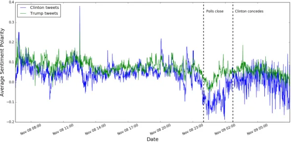
As a baseline, we will first use Pattern’s sentiment analysis algorithm, which returns a sentiment polarity between -1 and 1 [10]. Figure 4-1 shows the average sentiment per minute during election day on November 8, 2016.

Figure 4-1: Average Sentiment during the 2016 Presidential Election

dotted line indicates Hillary Clinton’s concession. Clinton and Trump had similar sentiment trends during the course of the election night. The average sentiment polarity for both candidates remained fairly stable at around 0.1 until polls closed. The average sentiment then dropped for both candidates after the polls closed and then started to stabilize after Clinton’s concession.

Compared to tweets about Trump, the average sentiment for Clinton dropped more after the polls closed and remained more volatile after her concession. Even though we can identify differences in sentiment, it is still difficult to draw conclusions on how the public’s attitude towards Clinton and Trump evolved throughout the election, since a wide variety of emotions are associated with a negative sentiment.

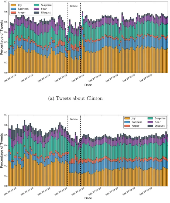
In contrast, figure 4-2 shows how the emotion distributions shifted throughout the night in ten-minute intervals. After the polls closed and it became clear that Trump had accumulated most of 270 electoral votes required, anger quickly became the predominant emotion in tweets about Clinton. After Clinton’s concession to Trump, the predominant emotion then changed to sadness for Clinton.

Figure 4-2: 2016 Election Day Emotion Distributions

(a) Tweets about Clinton

(b) Tweets about Trump

Interestingly, the emotion distributions after these key events did not appear to fluctuate as much for tweets about Trump, even though it is expected that the per-centage of "joy" tweets would increase for Trump after Clinton’s concession. One possible explanation is that the demographics of Twitter users are not totally

repre-sentative of the average US voter, since social media appeals more to young users, who have historically been more likely to support the Democratic party [15].

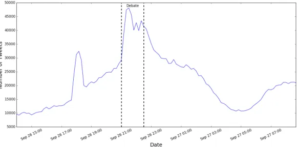
4.2.3 Using Volume to Identify Events

Next, we analyzed tweets from the first presidential debate. George Washington Uni-versity’s dataset includes tweets from a 24-hour period starting from the morning of each presidential debate and ending the next morning after the debate had con-cluded. In figure 4-3, we plot the number of tweets aggregated over each ten-minute window throughout this 24-hour period. As expected, the number of tweets spikes dramatically during the debate, which occurred from 9:00 PM - 10:30 PM Eastern time (marked by the dotted lines). We also see that the relative frequencies of each Ekman emotion remain relatively stable before and after the debate, but greatly fluc-tuate during the debate. Thus, using a combination of Twitter volume and changes in sentiment can potentially be used to identify unusual events that occur during a given time period. This topic will be explored further in chapter 5 in the context of financial tweets. Since major current events often lead to volatility in the stock market, we will now investigate the impact of presidential debates on future stock returns.

Figure 4-3: First Presidential Debate

(a) First Presidential Debate Tweet Volume

4.3 Can Presidential Debates Predict Market

Re-turns?

Oehler et al. previously found that the stock returns for related sectors and indus-tries following a presidential election were highly correlated with the new president’s policies [35]. In this section, we aim to determine whether this observation also holds true after presidential debates. We will analyze the predicted impact of Clinton and Trump’s proposed policies on a subset of S&P 500 industries and compare the stock market reaction immediately following each debate.

4.3.1 Summary of Candidate Policies

Here we will briefly summarize Clinton and Trump’s contrasting policies relating to a subset of S&P 500 sectors and industries.

∙ Pharmaceuticals and Biotechnology: Clinton proposed tighter regulations on drugmakers and wanted to set monthly price limits on drugs, both of which would lead to a loss of profits for pharmaceutical companies. Trump also wanted to make drugs more affordable, but was not as detailed about his plans. There-fore, the pharmaceuticals industry was predicted to perform better under a Trump administration [14].

∙ Financials: Clinton proposed tighter regulations on banks, so the financials sector was also predicted to perform better under Trump [5].

∙ Energy: Trump planned to lift restrictions on oil and gas companies, and increase fossil fuel production to increase job growth opportunities. Clinton’s policies focused on renewable energy. Since the majority of stocks in the Energy sector are oil and gas companies, Trump’s election was predicted to benefit the Energy sector [4].

∙ Defense: The Defense industry would benefit from a Trump presidency due to his plans for increased defense spending [5].

∙ Technology: The Technology sector would perform better under Clinton due to her support for highly skilled immigration and plans to increase spending on STEM education [47].

∙ Healthcare Facilities: Trump wanted to repeal and replace the Affordable Care Act, which would create a lot of uncertainty for hospitals. Therefore, healthcare facilities and hospitals would benefit from a Clinton presidency [23].

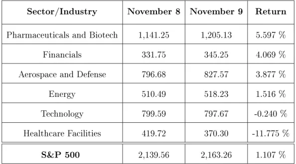
4.3.2 S&P 500 Returns after Election Day

Table 4.1 shows the closing prices and returns for each of these sectors on November 9, 2016, the day after the election. As predicted, pharmaceuticals, financials, defense, and energy made large gains after President Trump was elected. Healthcare facilities also fell significantly while the technology sector fell slightly, confirming Oehler’s observations about the impact of presidential elections on specific sectors.

Table 4.1: S&P 500 Sectors before and after Election Day

Sector/Industry November 8 November 9 Return Pharmaceuticals and Biotech 1,141.25 1,205.13 5.597 % Financials 331.75 345.25 4.069 % Aerospace and Defense 796.68 827.57 3.877 % Energy 510.49 518.23 1.516 % Technology 799.59 797.67 -0.240 % Healthcare Facilities 419.72 370.30 -11.775 %

S&P 500 2,139.56 2,163.26 1.107 %

To determine whether this pattern also holds true for presidential debates, we will use our emotion classifier to determine winners for the presidential debates.

4.3.3 Who won the Presidential Debates?

We will now analyze the changes in emotion distributions to predict a winner for each of the three presidential debates. Figure 4-4 shows the emotion distributions before and after the first presidential debate (marked by the black dotted lines) for both presidential candidates.

Figure 4-4: Emotion Distributions during the First Presidential Debate

(a) Tweets about Clinton

We can see that the percentage of joy tweets for Clinton increased after the debate, while the percentage decreased for Trump. Thus, we will use the change in percent-age of joy tweets to estimate how each debate affected public opinion towards both candidates. Tables 4.2 and 4.3 display the percentage change in tweets expressing joy before and after each presidential debate for Clinton and Trump, respectively.

The percentage of positive tweets increased for Clinton after all debates and it decreased after all debates for Trump. Therefore, based on our emotion distributions, we can conclude that Clinton’s performances on all three presidential debates were better-received than Trump’s.

Table 4.2: Clinton: Change in joy tweets before and after debates Before After Change

First Debate 21.467 % 23.411 % 1.944 % Second Debate 13.504 % 18.202 % 4.698 % Third Debate 15.304 % 21.986 % 6.682 %

Table 4.3: Trump: Change in joy tweets before and after debates Before After Change

First Debate 17.136 % 15.937 % -1.199 % Second Debate 17.013 % % 15.839 % -1.174 % Third Debate 16.211 % 14.845 % -1.366 %

These results are supported by the polls that Morning Consult conducted after the conclusion of each debate (Table 4.4). All three polls showed that a higher percentage of participants believed that Clinton was the winner of each debate [12] [36] [13].

Table 4.4: Morning Consult Poll Results Clinton Won Trump Won First Debate 49 % 26 % Second Debate 42 % 28 % Third Debate 43 % 26 %

4.3.4 S&P 500 Reactions to Presidential Debates

Now we will evaluate whether there is any correlation between Clinton’s debate wins and stock returns for industries relating to her major policies. Table 4.5 shows S&P 500 returns following the first presidential debate. Technology stocks gained 1.15% and energy stocks fell in response to Clinton’s win, as we predicted in the above section. The other four industries also made small gains.

Table 4.5: S&P 500 Industries Before and After First Presidential Debate Sector/Industry September 26 September 27 Return

Technology 790.18 799.26 1.15 % Financials 316.87 319.60 0.862 % Pharmaceuticals and Biotech 1224.38 1232.88 0.694%

Aerospace and Defense 783.44 786.82 0.431 Healthcare Facilities 402.76 404.26 0.372 %

Energy 495.00 492.72 -0.461 % S&P 500 2,146.10 2,159.93 0.644 %

However, the industry-specific returns following the second debate do not seem to be correlated with Clinton’s policies, as energy stocks rose significantly after the second debate (Table 4.6). Nevertheless, the overall S&P 500 index still rallied follow-ing the first and second presidential debates, which is another predicted result based

on the similarity of Clinton’s policies to those of the incumbent president, Barack Obama, as Prechter had previously found a positive relationship between an incum-bent’s vote margin and the percentage gain in the stock market during the three years prior to the election [39].

Table 4.6: S&P 500 Industries Before and After Second Presidential Debate Sector/Industry October 7 October 10 Return Healthcare Facilities 399.31 407.94 2.161 % Energy 520.28 528.11 1.505 % Technology 800.80 806.31 0.688% Financials 325.70 327.33 0.500 % Aerospace and Defense 774.73 777.31 0.333 % Pharmaceuticals and Biotech 1,217.21 1,219.32 0.173 % S&P 500 2,153.74 2,163.66 0.461%

Likewise, after the third debate (Table 4.7), pharmaceuticals gained, technology stocks fell, and the S&P 500 index also fell, contradicting Clinton’s proposed poli-cies. However, the third presidential debate occurred around the same time as many earnings announcements, which could explain some of the unexpected returns [24].

Table 4.7: S&P 500 Industries before and after Third Presidential Debate Sector/Industry October 19 October 20 Return Pharmaceuticals and Biotech 1,170.89 1,175.90 0.428 % Healthcare Facilities 430.72 432.08 0.316 % Financials 326.25 326.19 -0.018 %

Energy 520.89 520.41 -0.092 % Aerospace and Defense 775.66 774.32 -0.173

Technology 799.21 797.35 -0.233 % S&P 500 2,144.29 2,141.34 -0.138 %

4.4 Discussion

Even though we were unable to identify a clear pattern between presidential debate winners and stock returns for related S&P 500 industries and sectors, we have still shown that categorizing tweets into emotions is more effective than a polarity-based approach at highlighting differences in public opinion towards presidential candidates. Oehler’s study also concluded that abnormal returns after elections are probably caused by initial uncertainty towards the new president’s policies [35]. Even though Clinton performed better in all three debates, Clinton’s policies were still just theo-retical at the time. Other economic factors, such as earnings announcements and the state of the global economy, may also overshadow the impact of presidential debates on the stock market.

Furthermore, participants who believed that Clinton won the debates may have still disagreed with some or all of her policies. The first poll conduced by Morning Consult showed that even 12 % of Trump supporters believe that Clinton won the debate [12]. Thus, in addition to categorizing tweets by the presidential candidates mentioned, it would also be interesting to analyze the sentiment of tweets about

Chapter 5

Emotion Analysis of Financial Tweets

In 2012, Twitter introduced cashtags, which are stock ticker symbols prefixed with a $ symbol that behave similarly to hashtags. Cashtags can be used to search for financial news about publicly traded companies. In this chapter, we will explore the relationships between the sentiment and volume of tweets tagged with NASDAQ-100 cashtags and future returns for NASDAQ-100 companies.

5.1 Datasets

Tweets were obtained from Enrique Rivera’s NASDAQ 100 Tweets dataset published on Dataworld. This dataset contains approximately 1 million tweets mentioning any NASDAQ-100 ticker cashtag symbols between March 10, 2016 and June 15, 2016 [41]. However, most ticker symbols were missing data at the beginning of this period, so we only used tweets starting from March 28, 2016. This dataset also contains additional metadata for each of the 100 cashtags, such as the most retweeted tweets and the top 100 Twitter users sorted by number of followerss.

We also used Yahoo Finance to obtain daily adjusted closing prices during this three-month period. Millisecond trade data was obtained from the Wharton Research Data Services (WRDS) TAQ database. Earnings announcement dates and estimates were obtained from Zacks Investment Research.

5.2 Correlation Between Emotions and Stock Prices

Previous work by Zhang suggested that emotional outbursts of any type on Twit-ter had weak negative correlations with future Dow Jones, S&P500, and NASDAQ index prices [56]. We want to investigate whether focusing only on financial tweets tagged by cashtags, instead using a sample of all tweets as Zhang did, would produce a stronger correlation with future stock market performance. First, we calculated the distribution of Ekman emotions on each day over all cashtags in our dataset using the emotion classifier we described in Chapter 3. Then, we calculated the Pear-son correlation coefficients between the percentages of each Ekman emotion and the NASDAQ-100 return on the next day.

The Pearson correlation coefficient (Equation 5.1) is a measure of the strength of the linear relationship between two variables [34]. 𝑟 can range between -1 and 1, where 1 represents a perfect positive linear correlation, 0 represents no linear correlation at all, and -1 represents a perfect negative linear correlation. We used the percentages of each emotion on day 𝑡 as 𝑥 and the return corresponding to the price change from day 𝑡 to day 𝑡 + 1 as 𝑦. 𝑟 = ∑︀𝑛 𝑖=1(𝑥𝑖− ¯𝑥)(𝑦𝑖− ¯𝑦) √︀∑︀𝑛 𝑖=1(𝑥𝑖− ¯𝑥)2 √︀∑︀𝑛 𝑖=1(𝑦𝑖− ¯𝑦)2 (5.1) Since anyone can make a Twitter account and post random tweets containing cashtags, we also wanted to determine whether tweets from more reliable sources were more predictive of future returns. Thus, we also collected tweets only from the top 100 Twitter users sorted by number of followers and calculated the correlation coefficients again for this subset of tweets for all NASDAQ-100 stocks. Table 5.1 displays the average correlation between the emotion percentages and each stock’s return on the following day, for both all tweets and only tweets written by the top 100 users. Since surprise can be either a positive or negative emotion, depending on the type of news, we also calculated separate correlation coefficients between "surprise" tweets with a positive polarity score and surprise tweets with a negative polarity score. Bolded values are statistically significant at 𝑝 < 0.10.

We found that none of the original Ekman emotions had statistically significant correlations with next-day returns for either of the two groups, with all correlation coefficients being under 20 percent. However, tweets expressing positive surprise and negative surprise from the top 100 users showed stronger positive and negative cor-relations, respectively. This could be because uncertainty usually leads to volatility in the stock market, as shown during the aftermath of the 2016 presidential election. Therefore, using a combination of sentiment polarity and finer-grained emotion clas-sification can reveal more information about future stock returns than either of these approaches alone.

Table 5.1: Correlation between average emotion percentages and next-day stock re-turns

Emotion Top 100 Users All Users Joy 0.0763 0.0963 Fear -0.0864 0.0109 Sadness -0.0094 0.0050 Disgust -0.1127 -0.0779 Anger -0.1389 -0.0971 Surprise 0.1999 0.0395 Surprise (positive) 0.2780 0.0914 Surprise (negative) -0.2383 -0.1978 No Emotion 0.1641 0.0620

We then calculated the correlations between the current day’s emotion percentages and the current day’s returns to determine whether twitter users are actually reacting to changes in stock prices instead. Table 5.2 shows the average correlation between each stock’s emotions and the return on from the same day. Interestingly, the top 100 users did not have significant differences in the correlations between same-day and next-day returns. In contrast, the general public had a much stronger positive

correlation between tweets expressing joy and also a much stronger negative corre-lation between tweets expressing anger. Both of these correcorre-lation coefficients were statistically significant at 𝑝 < 0.05. These results suggest that the general public is more reactive to stock market prices, while the top users have more neutral attitudes. This could be explained by the fact that many of the top users by follower count are professional news sources, such as Reuters, Wall Street Journal, and Business Insider. Thus, most tweets by these accounts would focus on reporting news about companies in an unbiased manner. In the future, it may be interesting to analyze sentiment in tweets posted by professional investors to determine whether it is possible to leverage expert opinions to predict changes in stock prices.

Table 5.2: Correlation between average emotion percentages and same-day stock returns

Emotion Top 100 Users All Users Joy 0.1535 0.3039 Fear -0.0073 -0.1075 Sadness -0.0996 -0.0814 Disgust -0.1383 -0.0083 Anger 0.0778 -0.2573 Surprise 0.1923 0.0474 Surprise (positive) 0.2110 0.3008 Surprise (negative) -0.1619 -0.1938 No Emotion 0.2128 0.1148

Excess noise in the Twitter dataset is another factor that could explain the low correlation values for emotions other than surprise. Zhang’s study was conducted in 2009, when there were only 18 million Twitter users, compared to over 300 million today [53]. Table 5.3 shows several examples of noise in the Twitter data. Many tweets contain multiple cashtags, even when not all of the companies are actually

discussed in the tweet.

Table 5.3: Noise in $AAPL Tweets

Tweet Emotion Polarity

Bad News For Twitter Longs https://t.co/yGVdirvJUD $AAPL #APPLE $DIS $GOOG $GOOGL $SQ $TWTR

sadness -0.7

Fitbit Management Upbeat on Expected New Product, Says Raymond James - Tech Trader Daily - $FIT $GRMN $AAPL https://t.co/aNFotcme9b

joy 0.109

Florida to face flooding, dangerous seas from Trop-ical Storm Colin #TRUMP $TWTR $AAPL #wlst https://t.co/vYHi5qLVya https://t.co/A5f0SckYxn

fear -0.6

RT @CamilleHurn: Classic Marxist economics about how a servile population will submit to any old crap $AAPL https://t.co/Ur5kShoS9V

disgust -0.178

Even though all of these tweets contain the $AAPL cashtag and are labeled with the correct emotion, none of the tweets are actually related to Apple. The first and second tweets are expressing emotions towards Twitter and Fitbit respectively, while the last two tweets do not mention any NASDAQ-100 company at all. The prevalence of these types of tweets can skew the emotion distributions and mask patterns and correlations that may be present.

Nevertheless, many previous studies have shown that Twitter volume has a greater impact on future stock prices, so we will explore this relationship in the next section.

5.3 Using Volume to Identify Events

In the previous chapter, we saw that Twitter volume spiked while a presidential debate was ongoing. We use a similar approach here to determine whether there is a correlation between tweet volume and stock returns. Spikes in Twitter volume can

indicate that a significant event has occurred, such as an earnings announcement, acquisition, or new product release. The stock market response to these events may either be positive or negative, depending on the nature of the event.

For instance, figure 5-1a shows the daily Twitter volume for the $MSFT cashtag and the daily returns for the Microsoft stock. There are two main spikes in volume during this three-month period. The first spike occurred on April 21, 2016, which was the date of Microsoft’s first quarter earnings announcement. Microsoft missed price targets by 2 cents per share, causing shares to fall by up to 5 percent in after hours trading [21]. The second spike occurred on June 13, 2016, when Microsoft announced its planned acquisition of LinkedIn that morning [44]. While LinkedIn’s share price increased by 47 percent, Microsoft’s stock price fell by 3.2 percent and remained relatively flat afterwards. Experts suggest that this negative response could have results from Microsoft’s poor track record with prior large acquisitions, including Skype and Nokia, which were not as successful as analysts had hoped [49].

On the other hand, figure 5-1b displays the daily Twitter volume and returns for Facebook. In contrast to Microsoft, the response to Facebook’s first quarter earnings announcement was overwhelmingly positive. Facebook crushed analysts’ earnings expectations, beating revenue expectations by a whopping 15 cents per share. Consequently, shares rose by 9 percent in the hours following Facebook’s earnings announcement on April 27, 2016 [46]. These observations suggest that we can use Twitter sentiment to predict whether a particular event will result in a positive or negative effect on a company’s stock price.

Figures 5-1c and 5-1d show the daily tweet volumes versus the percentage of tweets expressing a positive sentiment for each day. As we can see in figure 5-1c, the per-centage of positive tweets dropped on the day of Microsoft’s earnings announcement, while the percentage of positive tweets increased on the day of Facebook’s earnings announcement. Thus, it may be possible to construct a trading strategy that takes into account both the number of tweets and the sentiment on a given day to make decisions about whether to buy or sell certain stocks.

(a) MSFT Tweet Volume vs Returns (b) FB Tweet Volume vs Returns

(c) MSFT Tweet Volume vs Sentiment (d) FB Tweet Volume vs Sentiment

Figure 5-1: Twitter Volume Plots for Microsoft and Facebook

5.4 Sentiment-Based Trading Strategy

Now we propose a simple trading strategy based on Twitter volume and the percentage of tweets expressing joy. For simplicity, we will assume that the price of a stock does not change due to after-hours trading and that there are no additional fees associated with buying or shorting stocks.

We use a two-dimensional array to store daily returns for each of the NASDAQ-100 components in Rivera’s dataset. Let 𝑅𝑖,𝑡 represent the return for stock 𝑖 at time

𝑡. 𝑅𝑖,𝑡 =

𝑝𝑖,𝑡−𝑝𝑖,𝑡−1

𝑝𝑖,𝑡−1 , where 𝑝𝑖,𝑡 is the price for stock 𝑖 on day 𝑡. 𝑇𝑖,𝑡 and 𝐽𝑖,𝑡 represent

the total number of tweets for stock 𝑖 at time 𝑡 and the percentage of tweets labeled with the "joy" emotion at time 𝑡. 𝐶𝑖,𝑡 represents the amount of capital for stock 𝑖 at

time 𝑡 that is either currently invested or in the bank.

For each stock 𝑖, we keep track of moving averages for the total number of tweets and the percentage of tweets labeled with the "joy" emotion, using a rolling window of five days. This is because the trading week is five days and we only consider the Twitter volume and sentiment on days immediately preceding a trading day, so tweets

on Fridays and Saturdays are not included. Figure 5-1 also shows that there are fewer tweets tagged with cashtags on weekends since no stocks are traded and no company announcements are made.

We initially allocate $1 to invest in each NASDAQ-100 stock. To calculate the amount of capital on day 𝑡 (𝐶𝑖,𝑡), we need to consider the percentage of joy tweets

and the Twitter volume for day 𝑡−1. For each day 𝑡−1, if the total number of tweets (𝑇𝑖,𝑡−1) for a stock 𝑖 is at least one standard deviation greater than the previous week’s

average, this signifies that a noteworthy event may have occurred. Then we look at the percentage of joy tweets for that day. If the percentage of joy tweets (𝐽𝑖,𝑡−1) is

at least half a standard deviation greater than the previous week’s average, the event will probably result in a profit, so we will buy the stock when the market opens on day 𝑡 and then sell it after the market closes on day 𝑡. Thus, we gain a profit equal to the previous day’s capital times the daily return for stock 𝑖 on day 𝑡.

Likewise, if the percentage of joy tweets is at least half a standard deviation below the average, we will short the stock and repurchase it the next day. If neither of these conditions are satisfied, 𝐶𝑖,𝑡 will remain unchanged from the previous day. Equation

5.2 shows how the our calculation of the amount capital invested in stock 𝑖 varies based on our decision for day 𝑡.

𝐶𝑖,𝑡 = ⎧ ⎪ ⎪ ⎪ ⎪ ⎪ ⎨ ⎪ ⎪ ⎪ ⎪ ⎪ ⎩ 𝐶𝑖,𝑡−1* (1 + 𝑅𝑖,𝑡) if buying stock 𝐶𝑖,𝑡−1* (1 − 𝑅𝑖,𝑡) if shorting stock 𝐶𝑖,𝑡−1 otherwise (5.2)

5.4.1 Preliminary Results

Figure 5-2 shows the results of this strategy on Microsoft, Facebook, and Yahoo during this three-month period. The green lines represent the amount of capital using a baseline buy and hold strategy, while the blue lines show the results of our sentiment and volume based trading strategy. As shown in figures 5-2a and 5-2b, this