Analysis of truckload prices and rejection rates

(1)

Analysis of Truckload Prices and Rejection Rates

By

Yoo Joon Kim

B.Sc. Naval Architecture and Ocean Engineering, Seoul National University, 1999

Submitted to the Engineering Systems Division in Partial Fulfillment of the

Requirements for the Degree of

Master of Engineering in Logistics

at the

Massachusetts Institute of Technology

June 2013

0 2013 Yoo Joon Kim. All rights reserved.

The authors hereby grants to MIT permission to reproduce and to distribute publicly paper and

electronic copies of this document in whole or in part.

r

A

Signature of A uthor...

.

...

Master of Engineering in Logistics Program, Engineering Systems Division

May 30, 2013

C ertified by...

.

...

..

Dr. Chris Caplice Executive Director Center for Transportation and Logistics ,

//

Thesis Supervisor

A ccepted by ... ... ...

---Prof. Yossi Sheffi

Elisha Gray II Professor of Engineering Systems, MIT Director, MIT Center for Transportation and Logistics Professor, Civil and Environmental Engineering, MIT

(2)

Analysis of Truckload Rates and Rejection Rates

by

Yoo Joon Kim

Submitted to the Engineering Systems Division

in Partial Fulfillment of the

Requirements for the Degree of Master of Engineering in Logistics

ABSTRACT

Truckload (TL) is the principle mode of freight transportation in the United Sates. Buyers of TL services are shippers with significant amount of shipments throughout a year. Due to the complexity of their network and the large expenditure on transportation, shippers select their carriers through auctions and using optimization methods, and enter into long-term contracts with winners with the best prices. Shippers subsequently request their carriers to fulfill shipment every time there's a load, a procedure called 'tender'. Despite the sophisticated selection and the existence of contracts, shippers' tenders are frequently rejected by their carriers, a phenomenon called tender rejection. When this happens, the shipper has to find alternative carriers and most of the time the price for the load increases. With weekly rejection rate as a dependent variable, and with variability of volume, length of haul, or the differential in prices as independent variables, this research mainly used the linear regression method to examine how well these independent variables account for rejections for a given lane. The analysis used the data including TL shipment and tender records of 17 shippers for five years. This research also attempted to discover any geographic patterns of frequent rejections. The analysis of the relationship between truckload rates and rejection rates suggested a potential trade-off between price and rejection, which questions the generally accepted strategy of shippers minimizing truckload expenditures by unconditionally reducing rejections.

Thesis Supervisor: Dr. Chris Caplice

(3)

Acknowledgements

I am appreciative of those individuals that have assisted with my thesis research, as follows:

To my thesis supervisor, Chris Caplice, for his humbleness to answer to my very elementary

questions encouraging me to learn about the transportation industry and for his academic rigor

against complacency in analysis enriching my learning experience through this research.

To my thesis sponsor company, especially Kevin McCarthy and Steve Raetz, for always being

available to answer my questions and giving me valuable insights while analyzing the data.

To my MIT Supply Chain Management colleague, Jason Salminen for his help while editing the last

versions of my thesis paper.

(4)

List of Figures

Figure 1 Load volume by industry in dataset...

29 Figure 2 Load volume by length of haul...30

Figure 3 Load volume by origin ...

31 Figure 4 Load volume by destination ...

32 Figure

5 Load volume by tender depth ...

38 Figure 6 Average backup rate differential by tender depth...39

Figure 7 Quartiles of backup rate differential by tender depth ...

40 Figure 8 Quartiles of rejection rate by CV of weekly volume (bin)...

43 Figure 9 High rejection origins in the East North division...

44 Figure 10 High rejection destinations in the East North division...45

Figure 11 Average rejection rate by length of haul (2011)...

46 Figure 12 Rejection rate by distance in the East North Central division (2011) ...

47 Figure 13 Rejection in 100-125 mile distance range ...

48 Figure 14 Rejection vs. price in 100-125 mile distance range...

48 Figure 15 Quartiles of rejection rate by length of haul (bin) ...

49 Figure 16 Acceptance rate and rate differential by shipper ...

51 Figure 17 Acceptance rate and rate differential by customer by lane...

52 Figure 18 Quartiles of backup rate differential by rejection rate (bin)...53

Figure 19 Average linehaul rate by rejection rate (bin)...54

(7)

List of Tables

Table 1 Summary of results from previous research ...

28 Table 2 Origin and destination matrix ...

32 Table 3 Rejection rate on lane with volatile volume...

35 Table 4 Rejection rate and coefficient of variation of weekly volume ...

42

(8)

1 Introduction

Over-the-road trucking is the principal mode of domestic freight transportation in the United States. In 2011, the total trucking revenue amounted to $604 billion, contributing to 81% of the total U.S. commercial freight revenues (S&P 2013).

Within the trucking industry, the truckload (TL) transportation market is the largest segment, moving 33% of all shipments in the U.S. in terms of tonnage in 2011. TL service firms, or carriers, provide a full-truckload capacity for direct point-to-point shipment of goods based on shippers' demand. The buyers of TL services, or shippers, typically have large volume of freights throughout a year. Typically, TL service is offered based on long-term contracts, for one year or longer, between shippers and carriers.

Despite the significant role of TL transportation in the economy and the presence of long-term contracts, shippers frequently and consistently experience tender rejections in their day-to-day transportation operations. Tender rejection refers to an incident in which a carrier rejects a shipper's request for a shipment within a specific time window. When this occurs, the shipper must look for other available carriers, which often leads to sharp increases in transportation prices.

This thesis compares tender rejections in various conditions using actual market data, identifies the causes, and quantifies the impact of them. This section will introduce the truckload transportation industry, carrier economics and truckload price, shippers' procurement process of TL services, tender rejection and its impact on truckload price, and hypothetical reasons for the problem.

(9)

1.1 Trucking industry and segments

Shippers in the U.S. acquire truck transportation from the two main sources: private fleets and for-hire trucking firms. Thousands of companies operate their own truck fleet to fulfill their transportation needs. The

private-carrier market accounts for 49% of the total truck shipments (by tonnage) in 2011 with the remaining

51% filled by for-hire carriers (S&P 2013).

The for-hire trucking industry is further divided into the two segments: full-truckload (TL) and less-than-truckload (LTL). While both modes use the same transportation technology, e s s e ntially tractor-trailer trucks, they are different primarily by shipment size and service configuration (direct vs. consolidated). A typical TL

service transports a large single shipment (up to 40,000 pounds) for a shipper from a point of origin to a destination without intermediate stops. LTL carriers collect shipments of smaller sizes (typically 1,000 to 1,200 pounds per shipment) from multiple shippers and locations, and consolidate them into a full trailer for shipment between the carrier's terminals. Within the total for-hire market, TL accounted for 86% in 2011.

While this thesis is a study of tender rejection, which occurs only in the TL market, the scope of our analysis is limited to transactions of dry van carriers, the sub-segment of the TL market, where the problem is most prevalent. Dry van carrier involves the movement of general packaged merchandise and accounts for about the half of the TL market. The other half of the market is specialized carriers including heavy haulers, auto carriers, tankers, flatbed, bulk commodity, temperature-controlled, and others in the specialized category.

1.2 Major players of the truckload market

Shippers, carriers, and third party logistics providers (3PLs) are the three main players in the truckload industry.

(10)

Shippers are customers of TL carriers that own or control goods that need to be transported. Since TL service mostly involves consistent shipment over the course of a year, shippers in the TL industry are typically very large. A major packaged food company who needs to move millions of cans of food from the factory to various warehouses or retail distribution points is our typical TL shipper. Our problem, tender rejection, is also these shippers' problem, so our research was conducted from a viewpoint of shippers.

Trucking firms, commonly called carriers, provide TL service to shippers. They own or lease trucks and employ drivers. Carriers are also called second party logistics providers (2PLs) because, from the viewpoint of shipper, the carrier is a second party. The TL market is highly fragmented without a single dominant player, mainly due to low-entry barrier. There are around 45,000 carriers in the U.S. and the majority of them, around

30,000 of the total, have annual revenues of less than $1 million (S&P 2013).

3PLs are called non-asset-based carriers because they provide transportation services without owning any assets or employing any drivers. Again, they are called third party from a shipper's point of view. Leveraging their vast network and relationships with a number of asset-based trucking firms, 3PLs play a role as broker or

intermediary matching shipper's transportation demand with carriers' capacity. The role of 3PLs is crucial especially in the areas where overall truck volume is low and volatile and available trucks are scarce.

1.3 Truckload price

The price of truckload service mostly consists of two parts: linehaul rate and fuel surcharge. Price may also include accessorial charges if additional service, such as extra waiting time, is included. Since we analyzed transactions that involved no extra service, truckload price for this research is defined as,

truckload price = linehaul rate + fuel surcharge

(11)

1.3.1 Linehaul rate and LHPM

From the shippers' viewpoint, the price for the pure TL services is the linehaul rate. Thus, when we compared truckload prices in this research, we only referred to linehaul rates. Shippers pay linehaul rate based on the miles driven, with exception for short-haul shipments, which can be charged a sum per load. Hence, to compare truckload price for long-haul shipments between shippers, we used linehaul rate per mile (LHPM) as a benchmark.

Since the TL market is very fragmented and competitive, carriers' operating profit margin is very low and thus the truckload price reflects carriers' actual cost of providing TL services. Linehaul rate is priced so that it can compensate carriers' operating cost to serve the shipment, such as wages for drivers. Almost all long-haul TL drivers are paid based on loaded miles driven. Labor cost represents approximately one third of operating costs for carriers, on average, making it the single largest component of operating costs (S&P 2013).

Truckload price doesn't explicitly compensate for carriers' operating cost involved in empty miles. Empty miles are the distance a driver has to drive between the services (such as backhaul). Hence, in order to breakeven, a carrier should consider whether the linehaul rate covers the operating cost involved in driving both loaded and empty miles.

1.3.2 Fuel Surcharge

Shippers pay carriers a separate rate for the fuel cost involved in the shipment based on the market fuel price. The rate is called fuel surcharge (FSC). The most common FSC scheme is based on the difference between the prevailing market price of diesel fuel and a base rate set by the shipper (for example, $1.20/gallon). This difference in price is the price premium and it is calculated as,

fuel price premium = market fuel price - base rate

(12)

The FSC rate, which is charged based on miles driven, is calculated by dividing the price premium by truck's fuel efficiency as,

FSC rate = fuel price premium

truck'sfuel efficiency

Alternatively, the FSC rate is calculated by multiplying the fuel price premium by the FSC multiplier as,

FSC rate = fuel price premum x FSC multiplier

where the FSC multiplier is the inverse of fuel efficiency. The unit of FSC is $/mile.

Finally, the actual FSC for a load is computed by multiplying FSC per mile with the distance as,

FSC for a load = FSC x distance

Each shipper has its own FSC program with his defined base rate and fuel efficiency (or multiplier). Since a

FSC programs typically assumes the fixed fuel efficiency, it may benefit carriers who operate the trucks with

better fuel efficiency than the one defined in the FSC program.

The base rate, which is typically very low compared to market price, can be interpreted as carriers' burden for fuel cost.

1.4 Carrier economics

Carrier economics is the key to explaining carrier's responsiveness. In this section, we will discuss carrier economics and how it affects carrier's decision whether to accept or reject shipper's tender.

1.4.1 Connection cost

The TL carrier's cost can be divided into two parts: linehaul movement and connection to follow-on loads (Caplice & Sheffi 2003). Cost of linehaul movement equals to the operating cost involved in moving trucks

(13)

from a point of pickup to a destination, including wages, fuel, tires, etc. Cost of connection to follow-on load is the operating costs involved in deadheading and dwell time. Deadhead is movement of an empty truck from its current location to the location of the new load. Dwell time is the time the driver has to stay at a location waiting for a follow-on load to be identified. It also include the cost of waiting for loading and unloading at a facility.

While the cost of linehaul movement is well understood and controlled by carriers, cost of connection is never predictable with certainty by carriers. This is due to short tendering lead times (time between tender and pickup time) and the overall spatial and temporal variability of shipper demand.

1.4.2 Economies of scope

Due to the existence of a connection cost, the cost of serving a load highly depends on its follow-on load. Especially, the cost of serving two lanes (origin-destination pairs) by a single carrier can be lower than the cost that would be incurred by using two different carriers each serving a single lane. In this case, both the carrier serving the two lanes and shipper can benefit from economies of scope (Caplice & Sheffi 2003).

Such carrier economics may affect the carrier's decision. A carrier may reject a highly priced long-haul shipment if an empty backhaul is likely because the cost of connection to a potential follow-on load is too high. Even if an empty backhaul is highly likely, a carrier may accept short-haul shipments from an origin with consistent volume because he can expect with certainty that there is another load from the same origin when he returns during the same day.

1.4.3 Low entry barrier

The overhead cost for TL carriers is lower than that for most other modes of transportation because TL operations don't require large capital investment. The capital cost to purchase or lease trucking equipment represents the majority of the overhead cost.

(14)

Due to low overhead cost, TL carriers cannot always benefit from economics of scale. Operating two or more trucks doesn't give the carrier advantage over other carrier with one truck. This cost structure lowers barriers for local small carriers to enter into the market and makes the market highly competitive. Small carriers can always take business from larger ones by optimizing their business to a specific shipper.

Such lack of economics of scale is also applied to shippers. Simply buying large volume of truck services does not lower the overall price. Consistent volume, or having balanced volume coming in and out of its locations, allows carriers to lower their connection costs, thereby lowering truckload price for the shipper.

Excessive competition in the TL market can lead to tender rejection. A new carrier may win a shipper's business with low price. However, if the price doesn't reflect the carrier's cost of serving the business, then the carrier is likely to reject loads.

1.5 Procurement of truckload transportation

Procurement in general is the acquisition of goods, services or works from an external source. In the case of TL services, shippers acquire transportation services from for-hire carriers. The major part of TL service procurement is auction and carrier selection, especially for large shippers, who manage shipments over thousands of lanes. The result of auction and carrier selection is placed into the shipper's routing guide. When these major procurement processes are completed, the shipper's load manager uses the routing guide for execution of shipments on a daily basis.

In this section and also in the following literature review, we will divide the shipper's procurement processes into procurement and execution. The procurement starts from general transportation planning and ends with

(15)

the routing guide. Execution refers to managing each load on a daily basis following the instructions of the routing guide.

The following lists the main terms and processes at the procurement stage. In the following section, we will introduce issues in the execution stage with focus on tender rejection.

* Lane definition: A lane is an origin and a destination pair. Shippers often have consistent or large shipment volumes on some lanes, while having irregular or low volume on the other lanes. To attract potential carriers, shippers can define each lane at different levels of specificity, such as 'Napoleon, OH to Maxton, NC' (city to city) or '43545 to 28364' (5zip to 5zip). Such specificity depends on expected volume or variability. Carriers quote their TL service price based on shipper's lane definition.

* _{Reverse auction: To find the best carriers, shippers send a request for to potential carriers. The invited} carriers then bid with a price quotation for each lane. This is a reverse auction since the bidders are sellers of the service. TL auctions can also be private-value auctions in which bidders (carriers) bid based on their private value instead of common market value.

" _{Combinatorial auctions & package bids: Large sophisticated shippers accommodate carriers' package}

bids so they can lower the TL price by allowing carriers to capture the benefit of economies of scope. In this case, if a carrier can lower the overall cost by serving several lanes for a shipper, he will bid a competitive price for those lanes with the condition that the offer is valid only if he wins all of the lanes. This auction is a combinatorial auction because carriers can submit bids for a combination of lanes, rather than for individual lanes.

(16)

e WDP (winner determination problem): The WDP is simply the model used to select which carriers to assign across the shipper's network. This is typically a MILP with various constraints (e.g., max/min volume) or conditions (e.g., package bids).

e Primary carriers and primary rates: Winning carriers are assigned to each respective lane. Each winning carrier is called the primary carrier for that lane. To avoid confusion, there is only one primary carrier per lane used in this research. In practice, shippers can have multiple carriers for a lane in their routing guide. Truckload prices of primary carriers are called primary rates in this research.

" Routing guide: The output of the WDP is a carrier assignment which is placed in an electronic catalogue, commonly called a routing guide. Shippers manage their day-to-day transportation operation following their routing guides. When there is a shipment requirement, the shipper initially tenders the load to the primary carrier for the lane onto which the load falls. If the tender is rejected, a

new tender is extended to the next carrier in for the lane according to the routing guide. Logic for step-by-step procedures, such as tender interval time (e.g., 50 minutes) is also defined in the routing guide. The routing guide is part of TMS (transportation management system) software package that assist shipper's transportation management.

In this section, we reviewed shipper's sophisticated procurement processes using optimization methods. The

limitation of this method, however, is that the carrier selection is determined based on the shipper's expected volume for the planning period. Actual volume can be highly volatile or significantly different from the expectation at the time of auction. This volume variability may cause the carrier not to honor contracts by rejecting tenders.

(17)

1.6 Tender rejection

After completing procurement and populating routing guide with primary carriers, the shipper executes each load by tendering it to the primary carrier in day-to-day TL transportation management. Even though the shipper selects the best carriers for each lane using competitive auction, the primary carriers often reject the tenders.

1.6.1 Tender rejection, tender depth and backup carriers

Tender rejection occurs when the primary carrier cannot position a truck for the load. It can also happen when shippers tender an unplanned load, or a shipment occurs that is not on a lane defined in the routing guide. In this case, since the shipper doesn't have the primary carrier for the load, he extends the tender to carriers following the pre-determined logic in the routing guide defined for unplanned loads. Our research investigated mainly planned loads to discover the reasons for tender rejection by primary carriers.

Several tenders can be extended until the available carrier accepts the load. The number of rejections until the load is accepted is called 'tender depth'. For example, tender depth is '0' when the load is accepted by the primary carrier and it is '1' if the load is rejected by the primary carrier, but then accepted by the first available carrier. We refer to the secondary carriers as backup carriers. The final rate in the last tender that is accepted by the backup carrier is called the backup rate.

Throughout this paper, a load is classified as a rejected load if it is rejected at least once. Regardless of tender depth, all loads whose tender depth is 1 or higher are called rejected loads.

Shippers view the rejection rate of a carrier as an index of the carrier's performance. The rejection rate can also be applied to a specific lane, in which case the rate indicates the robustness of procurement (or routing guide) for the lane. Rejection rate is defined as,

(18)

rejection rate (of carrier) = number of loads rejected by the carrier

number of loads total tendered to the carrier

rejection rate (on lane) = number of rejected loads on the lane

number of total tendered load on the lane

for a given period.

Rejection rate can be computed for various time frames, such as annual rejection rate or daily rejection rate.

Acceptance rate is also used by shippers as a index for carrier's performance and it is defined as,

acceptance rate = 1 - rejection rate

1.6.2 Hypothetical reasons for tender rejection

Over the course of the contract period, misalignment between shippers' and carriers' network may lead to frequent tender rejections. Procurement was done based on the shipper's projection of transportation demand for the contract period. If shipper's actual demand deviates significantly from the plan, and if the change

affects the primary carriers' profitability, the shipper may face tender rejections more frequently. This issue can be addressed by periodically updating the routing guide based on a review of carrier performabce and by replacing bad performers with alternative carriers.

We hypothesized that, in day-to-day TL operations, the existence of the excessive connection costs, and the carrier's expectation of it, lead to tender rejections. For example, even if a load is profitable, the carrier may reject the load if the cost of connection to that load surpasses the profit. The carrier may also reject a load if they expect a long deadhead or dwell time following the tendered load. We also hypothesized that shortage of

for a given period

(19)

truck capacity contributes to tender rejection if the shipper's transportation demand for a specific lane rises sharply in a very short period.

These short-term factors are unpredictable and cannot be controlled by either carrier or shipper. However, we assume that there are factors that can be controlled by shippers based on our hypotheses for short-term carrier behavior. The factors that we examined in our research include load volatility on a specific lane, length of haul, and price or rate.

Even if a shipper has large volume over a lane for a year, if the daily or weekly volume is highly volatile, the primary carriers may not be able to provide capacity when demanded. This could lead to tender rejections.

Distance, or the length of haul, is potentially related to tender rejections because it can affect carriers'

equipment utilization. Distance is also a factor to the carriers' operational constraint: driver's hours-of-service

(HOS). By law a single driver can drive a maximum of 11 hours after 10 consecutive hours off duty. If a

carrier's driver is unable to finish the load within a day based on the driver's remaining hours of service, the tender for this load is more likely to be rejected. A shipment of over 600-mile distance also can pose an operational challenge for the carrier because it cannot be done in 11 hours. Distance matters especially for local or regional carriers. If a carrier has a limited shipper base, availability of follow-on load is highly unpredictable if the current load is long haul. Kafarski (2012) found that carriers reject more often if the distance exceeds 100 miles.

We assumed that contract price, or primary rate, also affects carriers' behavior. A carrier may serve several shippers and if the price of one shipper is higher than that of the other and the underlying costs are similar, then the carrier may reject the tender with lower price.

(20)

In the data analysis section, we will review whether these three factors in fact affected tender rejections in the actual transaction data.

1.6.3 Price escalation

A primary rate reflects the best possible price that the shipper can get for the lane during the procurement

period. Hence, it is expected that actual truckload price will increase from the primary rate when a tender for a shipment over the lane is rejected and the shipper has to confer to backup carriers. This is the reason why shippers try to minimize tender rejections.

1.7 Our research problem

Tender rejection has been the focus of much practical research (including studies in our literature review) because it makes transportation costs uncontrollable. This research extends the previous studies by examining various causal factors and quantifying their impacts on tender rejections. Especially, our research extends the study of Kafarski and Caruso (2012), which addressed the relationship between the length of the haul and tender rejections. We studied other factors such as price and volatility of lane volume.

In our research, we attempted to find more subtle relationships between truckload price and tender rejection. In many previous studies, tender rejection is always considered as a factor that raises truckload price and shippers' overall transportation expenditure. However, the relationship between tender rejection and truckload price itself has been rarely studied. Along the same line, high acceptance rate is implicitly considered good. However, we assumed that there is a cost for getting high acceptance.

We asked the following questions while analyzing data:

e Do shippers' demand volatility on lanes affect carrier response? e Does the length of haul affect tender rejection?

(21)

Should shippers whose goal is to minimize transportation cost aim at 100% acceptance rate?

1.8 Partner company

For this research, we partnered with C.H. Robinson Worldwide, a leading 3PL provider serving customers in freight transportation, mainly truckload trucking. Our dataset is provided by C.H. Robinson's TMC, a division of the company that provides outsourced transportation management. TMC manages truckload operations for over 40 clients, some of whom are the largest shippers in the U.S. Our dataset contains actual tender and shipment records of those clients over the past five years.

1.9 Looking ahead

The remainder of the thesis is organized as follows. Chapter 2 reviews previous research on truckload transportation with focus both on the procurement and on the execution aspects. Chapter 3 overviews our dataset and transportation network present in the data. This chapter also describes our key variable, weekly rejection rate. Chapter 4 exhibits our findings and what they suggest. The final chapter discusses the implications of our results for the TL shippers.

(22)

2 Literature Review

As a background to our research, we reviewed literature on various topics related to procurement of truckload services. The literature on this subject can be loosely categorized into two groups: procurement and execution. Studies in the procurement category addressed problems in shipper's procurement processes while research in the latter category focused on problems in day-to-day execution by analyzing shippers' actual tender and shipment data. Our research relates to execution. In this section, we will review research for both categories. We also summarize the key findings and insights from analysis of the previous research.

2.1 Truckload procurement

During the procurement process, shippers annually set up a transportation plan, hold an auction to obtain quotes from potential carriers, select carriers for each lane, and enter into annual contracts with each carrier. Finally, carrier assignments are placed into the shippers' routing guide for future execution. The previous research on TL procurement focused on optimization (a winner determination problem) and combinatorial auction.

2.1.1 Optimization-based procurement

Large shippers, who hold auctions to select carriers, have to solve complex optimization problems because they need to assign hundreds of carriers to thousands of lanes. Reynolds Metals Company was the pioneer in

using optimization to determine the winner of a transportation auction. Moore, Warmke, and Gorban (1991) described how Reynolds bid out and assigned lanes to carriers. Reynolds developed a mixed integer program model that minimized overall transportation costs by assigning carriers to each lane, taking into account individual carrier capacity constraints, volume commitments, and other constraints.

(23)

Caplice and Sheffi (2003) introduced the overall auction process for TL service procurement and carrier assignment methods using an optimization model. The authors discussed why economies of scope are more appropriate than economies of scale in explaining carriers' cost for providing TL service. They also described uncertainty in the bidding from carriers' perspective, due to the imbalance in the shippers' transportation network and the lack of information for carriers to predict the cost of doing business with the shipper.

Due to these uncertainties, carriers tend to hedge by raising their bids to a level much higher than their reserve price. Some carriers may also win a shipper's business with a bid that doesn't reflect the actual cost and then default on the contract. This is referred to as the 'winners' curse'. In both of the cases, uncertainty raises the shipper's overall transportation expenditure. To address this problem, the authors introduced an auction format that allows carriers to reduce uncertainties by bidding for a combination of lanes, instead of bidding for a single lane. Sheffi (2004) further explained how this combinatorial auction framework can benefit both shippers and carriers by exploiting economies of scope present in the TL industry, and also reported the case of actual implementations.

The authors provided lessons from practice. They explained the appropriate size of transportation network for optimization-based procurement versus manual analysis. The authors showed using an example that a shipper with 1,800 lanes and 200,000 loads per year, the optimization-based procurement reduced transportation cost

by 6%. They suggested what indices of carrier performance a shipper could factor into the optimization

method. They also discussed limitations of routing guide, as it cannot execute precisely upon the strategic plans that an optimization-based procurement process creates.

2.1.2 Routing guide

Caplice (2007) provided an overview of TL procurement with focus on routing guide. The author compared the terminologies used in TL procurement with the general terms used in a common electronic commerce format. Especially, routing guides correspond to the 'electronic catalogue' in the general electronic

(24)

marketplace format. Routing guide is also a synonym for transportation management system (TMS), which electronically executes tenders, selects carriers and manages payments.

Caplice (2007) connected various rules and considerations in TL procurement to actual mechanisms of the routing guide, such as the number of primary carriers assigned to a lane. Optimization methods yield one optimal carrier for each lane. However, shippers may assign two or more primary carriers to lanes with high volume. In such cases, the routing guide should have the logic to allocate each load to multiple carriers.

The author also explained the relationship between specificity of lane definition in TL procurement and assignment of a load to the primary carrier during execution using the routing guide. Caplice (2007) noted that shippers rarely include very specific lanes such as "5-digit postal code to 5-digit postal code" when putting lanes for an auction. Instead, shippers have multiple levels of lane specificity depending on load volume and variability. As a result, there can be multiple lanes in the routing guide with different specificities that can be applicable to a specific load. The routing guide should have the logic to tender to the right carrier to capture the benefit of the strategic procurement.

Caplice (2007) described a characteristic of a TL freight network; that most of load volumes are distributed on only a few lanes, while the majority of lanes have little volume. The network present in the dataset of this research had the same characteristic, limiting effectiveness of price comparisons among different lanes.

He pointed out that the contracts between shippers and carriers are not completely binding since carriers will not always have equipment available when the shipper requests it, while the shipper does not guarantee a minimum volume or dollar amount to the winning carriers.

(25)

2.1.3 Qualitative performance data into optimization problem

Harding (2005) discussed how to incorporate actual carrier performance metrics, such as rejection rate, into optimization methods. Optimization methods find a solution that minimizes the overall cost, taking into account the price of a carrier for a specific lane. Harding (2005) addressed issues with how to adjust carriers' bids before optimization so that carriers with a better acceptance rate are more likely to win the bid. He pointed out that a carrier's rejection rate should be viewed differently if the carrier rejected the shipper's unplanned load, as opposed to rejecting a planned load on the lane that the carrier is assigned to. Harding

(2005) also used simulation to show price escalation as a result of tender rejections.

2.2 TL shipment execution

Once strategic procurement is completed, shippers execute each shipment on a daily basis by tendering loads to primary carriers according to the routing guide and assigning them to the carriers who accepted them. In this section, we will review the previous studies that analyzed actual tender and shipment records. The researchers showed how the considerations used in procurement, such as a fuel surcharge program or lane definition, affected truckload prices. The rules in the routing guide, such as tender lead time, were also examined as a factor for variability in truckload prices.

2.2.1 Lane specificity and truckload price

Shippers typically define lanes based on an annual threshold volume (Caplice 2007). If a shipper has low volume on a lane, he uses a less specific lane definition such as "state to state," so that the lane includes larger volume. This exercise is called lane aggregation. Collins and Quinlan (2010) studied how lane aggregation affected transportation prices by comparing truckload price for different lane specificities such as point to point, point to region, and so on, where the researchers defined a 5-digit zip code as a point and any zone less specific than a 5-digit postal code as a region.

(26)

2.2.2 Fuel surcharge and truckload price

Each shipper has his own fuel surcharge program. A shipper compensates carriers for fuel costs that exceed the peg rate (in the introduction section, we called this base rate), which is usually set at $1.20 per gallon. With the knowledge of how much they will be compensated for fuel cost, carriers calculate their profitability for a specific lane and bid a price accordingly. Abramson and Sawant (2012) evaluated how a shipper's fuel surcharge program affected its linehaul rates and the result showed that carriers implicitly discounted their linehaul rates according to the shipper's surcharge program.

2.2.3 Tender lead time and truckload price

Caldwell and Fisher (2008) showed that longer lead time lowered variability of rates. Tender lead time is the time from when a shipper tenders a load to when the load needs to be picked up. The analysis showed that with a longer lead time that allowed carriers to have more time to plan for the load, shippers could reduce both truckload price and rejections.

2.2.4 Length of haul and rejection rate

Our research extends the work of Kafarski & Caruso (2012) on carrier rejection behavior and variability of truckload prices. They compared rejection rates on the transportation network of a large beverage company to identify over which lengths of haul range that rejections occurred more frequently. They used daily volume on a given lane (3-digit postal code origin to 3-digit postal code destination) to calculate rejection rates.

The analysis showed that the average daily rejection rate for a 9-month period varied by distance. The rates were near zero up to 100 miles, increased in the 100-400 mile range, and slightly declined from this peak for distances over 400 miles. It also showed that price escalations due to rejections were most severe in the

100-300 mile range, with the rate of increase ranging from 5 to 17%.

(27)

"We learned that they would usually round-trip equipment up to 100-140 miles and be willing to come back empty. However, beyond that distance, they would try to look for a backhaul load to still to make a profit. By going up

100-150 miles, carriers can complete around two loads a day, which provides them with optimal use of equipment. Then,

past the 400-mile mark, the situation again becomes more favorable to the carriers."

The researchers' interviews with various carriers also revealed that carriers reject tenders for the following reasons: short lead time, surge in volume, unplanned lane, long dwell time, adverse weather, inconsistent volume and low price.

2.2.5 Summary of findings of the previous research

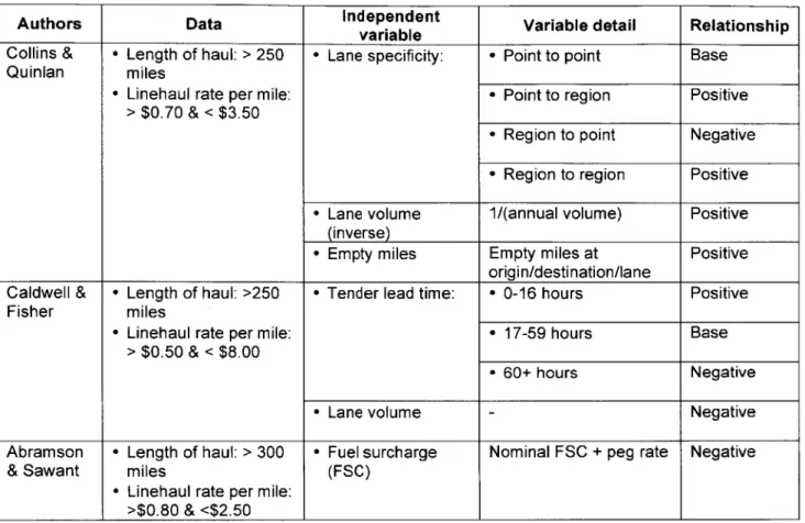
Table 1 lists the explanatory variables used in the previous research as described in section 2.2. The

"Relationship" column in the table indicates the correlation between the independent variables and truckload prices (dependent variable). For example, in Collins & Quilan's research, the lane specificity of the 'point-to-region' increased truckload price from the base case.

(28)

Authors Data Independent Variable detail Relationship variable

Collins & - Length of haul: > 250 - Lane specificity: - Point to point Base

Quinlan miles

e Linehaul rate per mile: - Point to region Positive

> $0.70 & < $3.50

- Region to point Negative

e Region to region Positive

e Lane volume 1/(annual volume) Positive

(inverse)

e Empty miles Empty miles at Positive

origin/destination/lane

Caldwell & - Length of haul: >250 - Tender lead time: - 0-16 hours Positive

Fisher miles

- Linehaul rate per mile: - 17-59 hours Base

> $0.50 & < $8.00

- 60+ hours Negative

- Lane volume Negative

Abramson - Length of haul: > 300 - Fuel surcharge Nominal FSC + peg rate Negative

& Sawant miles (FSC)

- Linehaul rate per mile: >$0.80 & <$2.50

Table 1 Summary of results from previous research

2.3 Chapter summary

We reviewed the previous research describing how shippers strategically procure TC services and select their primary carriers using optimization-based procurement methods that markedly lowered overall transportation costs. We also reviewed the research showing how various factors used in TL procurement affected truckload price and tender rejections in shippers' day-to-day transportation executions.

(29)

3 Dataset and Methodology

In this section, we will review our dataset and describe the truckload transportation network presented in the dataset. As the original dataset contained outliers and incorrect inputs, we will explain how we cleansed the data for analysis. To compare tender rejection in various conditions, it was essential for this research to adequately define the 'rejection rate' variable and we will explain why we used a weekly rejection rate.

3.1 The dataset

The dataset for this research included tender and shipment records for TL loads shipped during a period from

1/1/2008 to 9/30/2012. The dataset showed that 17 shippers made a total of 2,384,680 tenders to secure trucks

for 1,670,104 loads. The ratio of the number of tenders to the number of loads indicated that the shippers made 1.43 tenders on average to find the carriers.

(0 0 E z 1000K 800K 600K 400K 200K

Automotive Paper Manufactur-ing

Figure 1 Load volume by industry in dataset OK

Fooa &

Beverage

-M

(30)

The shipper group represented five market segments with the majority of the shipments belonging to the food

& beverage (59%) industry, followed by automotive (26%) and paper (8%) (Fig. 1).

Distance (Bin), miles 250K 200K 150K 0 50K

OKIhi

Er.E m 0D 0D 0 0 03 000 03 0C 0 0 0D 03 0 03 0 0D 0D 0 03 03 0 0 0 0D 0 0D 00 0CC - ' I U~' ) (0 f* U M ) ) - C'() ' U CD l-. W) M0) 0 r- "S () Iq to (0 I- M) M) oD

Figure 2 Load volume by length of haul

The carriers hauled an average of 467 miles for each load. The shipments that were greater than or equal to

100 and less than 400 miles contributed to 49% of the total and the short-haul shipments (less than 100 miles)

accounted for 12% of the total (Fig. 2). In general, shippers view the 100-400 mile length of haul range as the problematic range in which rejection is more likely than for shorter hauls (CHR 2013).

The truckload transportation network present in the dataset was countrywide. The origins and the destinations of the shipments extended over 49 states and over 3,000 cities. Over the five years, the shippers shipped goods over 17,000 lanes.

In our data analysis, lane is a paired origin and destination, both defined by 3-digit postal codes. It is important to note that only a very small percentage of the lanes were shared by more than one shipper even

(31)

though we broadly defined lanes using 3-digit postal codes. In 2011, the group of 17 shippers shipped their goods over 8,291 lanes. If all of the shippers shipped over the 8,291 lanes, the possible combination of lanes and shippers would total 140,947 (8,291 multiplied by 17). The actual combination in the dataset was only

8,581, which indicated that only very few lanes were shared by more than one shipper.

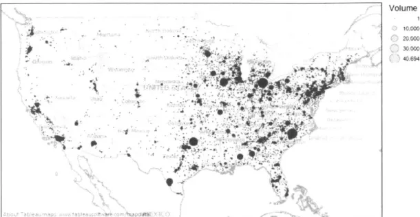
To compare the data by region, we divided the shipment records by the US Census Bureau's four regions and nine divisions (Fig. 3). The shipments with origins in the East North Central division of the Midwest region accounted for 26% of the loads, followed by the South Atlantic (14%), the Middle Atlantic (14%) and the West South Central (13%) divisions.

East South Middle

North Atlantic Atlantic Central West South Central Pacific West North Central

East Mountain New South England Central

Figure 3 Load volume by origin

Although the transportation network in the dataset extended throughout the country, it was only a fraction of the entire TL market in the U.S. in terms of transportation costs. The shippers' total expenditure in the dataset, based on linehaul rate and fuel surcharge, amounted to $337 million in 2011, which contributed to 0.12% of

0 0 E D' z 450K 400K 350K 300K 250K 200K 150K 100K 50K OK

(32)

*

4-'4

6 1 S. * ai *e * ,*,,, - ~" 2~J8I~ Volume 10.000 20.000 30.000 40.694

Figure 4 Load volume by destination

Destination East East Middle Moun- New South West West

North South Eng- Pacific . North South Sum

Origin Central Central Atlantic tai land Atlantic Central Central

East North Central 11% 1% 3% 0% 1% 0% 3% 5% 1% 26%

East South Central 1% 2% 0% 0% 0% 0% 4% 1% 1% 9%

Middle Atlantic 3% 1% 5% 0% 1% 0% 3% 0% 0% 14%

Mountain 0% 0% 0% 0% 0% 2% 0% 0% 0% 3%

New England 0% 0% 1% 0% 0% 0% 0% 0% 0% 2%

Pacific 0% 0% 0% 3% 0% 8% 0% 0% 0% 12%

South Atlantic 1% 3% 2% 0% 0% 0% 6% 0% 1% 14%

West North Central 2% 1% 0% 0% 0% 0% 1% 3% 1% 8%

West South Central 1% 1% 0% 2% 0% 0% 1% 2% 6% 13%

Sum 20% 8% 12% 6% 2% 11% 19% 10% 11% 100%

Table 2 Origin and destination matrix

3.2 Data preparation

In this section, we will review how we cleansed the dataset and normalized the linehaul rate. We will also discuss why we used a weekly rejection rate to compare tender rejections in various conditions.

(33)

3.2.1 Data cleansing

The initial dataset included input errors and outlying figures, mostly due to manual inputs by the load planners at the shippers. Abnormal linehaul rates were filtered out by using the following criteria:

* 0 < Distance <= 250 miles AND Linehaul rate > $800

- Distance > 250 miles AND Linehaul rate per mile (LHPM) > $3.20/mile e LHPM < $0.70/mile

The following incorrect inputs and out-of-scope data were also excluded from our dataset: * Distance equal to or less than zero

e Customer (shipper) ID "NA"

e Incorrect origin and destination zip codes

- StopQuantity not "1 P1 D" (shipments with more than one pickup or drop points) e Mode not "Van TL" (non dry-van shipments)

e "Expedited" ('expedited' service for extra charge) - The number of accepted tenders per load more than one - Tender sequence not starting from 0

Appendix A.1 includes details of the data field in our dataset.

3.2.2 Normalized linehaul rate

In this research, we compared only linehaul rates to evaluate differences in truckload prices. To correctly compare linehaul rates of multiple shippers, we normalized the linehaul rates by eliminating the differences in fuel surcharge rates among the shippers.

(34)

total rate = linehaul rate + fuel surcharge

and computed normalized fuel surcharge by,

normalized fuel surcharge = (market fuel price - base price) x multiplier

We applied the same base price of $1.20 per gallon and the same multiplier of 0.17 gallon per mile to all of the shipments in the dataset. The multiplier implies the truck's fuel efficiency of 5.88 mile per gallon.

Finally, the normalized linehaul rate is calculated by,

normalized linehaul rate = total rate - normalized fuel surcharge

3.2.3 Rejection rate

The rejection rate indicates how frequently tenders are rejected for loads on a given lane. It is computed by,

rejection rate = number of rejected loads

number of total loads

for a given lane.

In our analysis, we also used acceptance rate as a criteria to measure carrier's responsiveness to shippers' tender and it is computed by,

acceptance rate = 1 - rejection rate = number of accepted loads

number of total loads

It is important to note that we used a weekly rejection rate to mitigate the effect of high volatility of daily load volume. For example, Table 3 shows that the daily rejection rate for a hypothetical lane swings between 5% and 100%. The average of the daily rejection rates for this week is,

(35)

5% + 100% + 5% + 100% + 5%

5 =43%

This average (43%) indicates that rejection rate for this lane was much higher than normal. However, the shipper experienced rejection relatively not so frequently compared to the total number of loads during this week. The average is high because it assumes each day is equal.

Day Mon Tue Wed Thu Fri

Number of loads 20 1 20 1 20

Rejected loads 1 1 1 1 1

Daily rejection rate 5% 100% 5% 100% 5%

Table 3 Rejection rate on lane with volatile volume

On the other hand, the rejection rate based on the weekly volume is,

1+1+1+1+1 5

= - = 8.06%

20+1 + 20+ 1 + 20 62

We considered that the weekly rejection rate is a better indicator of a tender rejection problem for this

hypothetical lane. Using weekly rejection rates was more appropriate for our dataset because most of the lanes in the dataset had highly volatile volume.

3.3 Regression analysis

In this research, we used the regression analysis to find the relationships between rejection rate and the explanatory variables that we expected to account for rejections.

We used the simple linear regression to examine each of the two key independent variables for this research: variability of load volume and length of haul. The linear regression model assumes that

(36)

Y = fo + / 1x + E

where E is a Normally distributed random variables with mean i = 0 and some unknown standard deviation o.

x is the independent or explanatory variable and Y is the dependent variable.

We mainly looked at the R squared, or the coefficient of determination, of the regression results to see how well the explanatory variables explain rejection rates, the dependent variable. The R squared is the proportion of total variation of the observed values of the dependent variable Y that is accounted for by the regression equation of the independent variable x.

(37)

4 Data Analysis

Our analysis showed that tender rejections mostly led to increased truckload prices, resulting in excess planned transportation expenditures for shippers. We examined the three explanatory variables that we expected to explain the tender rejection problem, including volatility of shippers' demand, length of haul, and shippers' price relative to the market price.

4.1 Rejection and price escalation

During the five-year period of our dataset, 1,071,218 loads, or 64% of the total shipments, were planned, thus these planned loads were tendered to the primary carriers according to each shipper's routing guide.

Throughout this section, a planned load refers a shipment over a defined lane (as per the shipper's routing guide) along with the primary carrier and the primary rate.

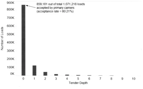
Of the total planned loads, the carriers rejected 212,037 loads, yielding the aggregate rejection rate of 19.8%

(Fig 5). For the entire planned loads, the shippers' total expenditure amounted to $799 million, based on the primary prices. Due to rejection, the shippers paid an extra $23 million, or 2.8% more.

For the rejected loads alone, the shippers paid on average 14.8% above their primary prices. However, not all of the rejected loads resulted in increased prices. 29,444 loads, or 13.9% of the rejected loads, experienced an average price decrease of 10.4%. For the remaining rejected loads, the price increased by an average 19.2% on average. For those loads that were rejected (but the backup rates were lower than the primary rates), no specific patterns, such as certain regions, length of haul, or certain times of a year, were observed.

In Fig. 5, the tender depth indicates the number of rejections the shipper experienced for a load before the final backup carrier accepted the load. The tender depth "0" indicates that there was no rejection since the

(38)

primary carrier accepted the tender. The tender depth "2" indicates that two carriers including the primary carrier rejected the load until the second backup carrier accepted it. In this research, all of the loads with tender depth of I or higher were regarded as rejected loads. The backup carrier is the carrier who was tendered a load after the primary carrier rejected it and the backup rate is the rate at which the final backup carrier accepted it. As the data suggested, backup rates are usually higher than the respective primary rates.

While the dataset included loads with tender depth up to 58, the chart in Fig. 5 was truncated at the tender depth of 10, as the loads above this level accounted for only 0.2% of the total. Most of the rejected loads were accepted by the first or the second backup carriers (78% of the rejected loads).

(0 ('3 0 E z 900K 800K 700K 600K 500K 400K 300K 200K 100K OK

859,181 out of total 1,071,218 loads accepted by primary camers (acceptance rate = 80.21%) 3 4 5 6 Tender Depth 7 8 9 10 II2 0 1 2

Figure 5 Load volume by tender depth

The average backup rate differential increased by tender depth (Fig. 6). Backup rate differential for a load is defined as,

backup rate differential = backup rate - primary rate primary rate

(39)

Tender depth may indicate the shortage of available backup carriers at the time of the tender, since the deeper the tender, the longer the time or more effort for the shipper to find the backup carrier. High tender depth may also indicate a shortage of carriers at the tendered price and in such cases the shipper should increase the price to attract backup carriers.

0 0 4 0 (U (D 0.3 0 0 0.2 0.1 0 0 0 0 00 0 2 3 4 5 Tender Depth 6 7 8 9 10

Figure 6 Average backup rate differential by tender depth

The regression analysis showed the relationship between tender depth and backup rate differential as,

backup rate differential = 13.18% + 3.09% x tender depth + error

where,

tender depth = 1, 2, 3, ...

In the analysis, the dependent variable was the backup rate differential of each load and the dependent variable was the tender depth of each load. The loads that were accepted by the primary carriers were excluded from the regression.

(40)

The weak R squared of 1.62% suggested tender depth alone was not a good indicator of change in backup rate differential and that other variables caused backup rates to rise from the primary rates.

0.6 -j 0.5 C 0.4 6 0.3 a 0.2 0.1 0.0

Tender Depth (bin)

0.00 -A

0

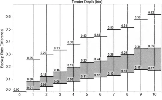
Figure 7 Quartiles of backup rate differential by tender depth

The shippers in the dataset had three carriers assigned to each lane. The rates of the second and third carriers were mostly higher than the rate of the first carrier (primary carrier). Hence, the rates for the tender depth of 4 and above, could have been affected by various factors. Different tender sequencing logic or tender lead time also could have accounted for backup rate differential. For example, for the load with the tender depth of 58 in the dataset, the shipper allowed a long lead time of 8 days, making 7.3 tenders a day on average, eventually finding a backup carrier whose rate was lower than the primary rate.

As Fig. 7 shows, the backup rate differentials varied widely even for the same tender depth. For the loads with tender depth of 3, for example, the backup rate differentials between the upper and the lower quartiles ranged from 6% to 33%.

Analysis of truckload prices and rejection rates

ARCHIVES