Analysis of and techniques for adaptive equalization for underwater acoustic communication

Analysis of and Techniques for Adaptive Equalization

for Underwater Acoustic Communication

by

Ballard J. S. Blair

Submitted to the

Department of Electrical Engineering and Computer Science in partial fulfillment of the requirements for the degree of

Doctor of Philosophy at the

MASSACHUSETTS INSTITUTE OF TECHNOLOGY

MASSACHLiSETTS INSTITUTE OF TEr:fJCHNLOGY

SEP 2 7 2011

LRARIES

ARCHIVES

WOODS HOLE OCEANOGRAPHIC INSTITUTE September 2011

@

The author hereby grants to MIT and WHOI permission to reproduce and distribute publicly paper and electronic copies of this thesis document in whole or in part.

/

i

//)

4

11

A

A uthor ... .. . ... ( ... Joint Program in Oceanography

Certified by...

Accepted by...

...

/

... ... ... ... ...

James C. Preisig Associate Scientist, Woods Hole Oceanographic Institution Thesis Supervisor

Chair, Joint Committee

r'P)

Accepted by ...

A I

"nPI /

...

James C. Preisig for Applied Ocean Science and Engineering Massachusetts Institute of Technology/ j Woods Hole Oceanographic Institution

...

/ u Leslie Kolodziejski

Professor of Electrical Engineering Chairman, Department Committee on Graduate Theses Massachusetts Institute of Technology

Analysis of and Techniques for Adaptive Equalization

for Underwater Acoustic Communication

by

Ballard J. S. Blair

Submitted to the Department of Electrical Engineering and Computer Science on September 2, 2011 in partial fulfillment of the requirements for the degree of

Doctor of Philosophy in Electrical and Oceanographic Engineering

Abstract

Underwater wireless communication is quickly becoming a necessity for applications in ocean science, defense, and homeland security. Acoustics remains the only prac-tical means of accomplishing long-range communication in the ocean. The acoustic communication channel is fraught with difficulties including limited available band-width, long delay-spread, time-variability, and Doppler spreading. These difficulties reduce the reliability of the communication system and make high data-rate commu-nication challenging. Adaptive decision feedback equalization is a common method to compensate for distortions introduced by the underwater acoustic channel. Limited work has been done thus far to introduce the physics of the underwater channel into improving and better understanding the operation of a decision feedback equalizer. This thesis examines how to use physical models to improve the reliability and reduce the computational complexity of the decision feedback equalizer. The specific topics covered by this work are: how to handle channel estimation errors for the time varying channel, how to use angular constraints imposed by the environment into an array receiver, what happens when there is a mismatch between the true channel order and the estimated channel order, and why there is a performance difference between the direct adaptation and channel estimation based methods for computing the equalizer coefficients. For each of these topics, algorithms are provided that help create a more robust equalizer with lower computational complexity for the underwater channel.

Thesis Supervisor: James C. Preisig

Acknowledgments

A PhD thesis is a singulalry authored document, but not one that is written in isolation. Thank you to my advisor, Dr. James Preisig, for spending countless hours guiding this research and supporting this writing. He is truly dedicated to enabling his students to produce high quality, meaningful research.

Thank you also to my thesis committee for their generous assistance: Prof. Milica Stojanovic spent many afternoons pointing me back in the right direction; I am grateful for her time, tricks, and intuition. Prof. Arthur Baggeroer was generous with his expansive knowledge and diligent to make this an accessible document. Prof. Greg Wornell always had a unique perspective from which research problems had apparent solutions.

The members of my labs both at MIT and WHOI were great in working through research ideas and clarifying research presentations. I am grateful to the members of Dr. Preisig's research group, especially Joe Papp, Milutin Pajovic, Dr. Ananya Sen Gupta, Atulya Yellepeddi, Jared Severson, and Dr. Andrey Morozov for their keen insights. Thank you also to the members of the DSPG group, especially Zahi Karim, Tom Baran, Shay Maymon, Sefa Demirtas, and Dennis Wei for time, energy, and support. I would be remiss to not mention Jon Paul Kitchens for our weekly lunch discussions where many of these ideas were born.

Like a lost puppy, I wandered through many research homes at both MIT and WHOI. I am a better, more rounded researcher for having been exposed to all these different viewpoints. I am grateful to many people for support during my wanderings: Prof. Louis Whitcomb and James Kinsey who pointed me to the Joint Program; Dr. Hanu Singh and Prof. Daniela Rus who gave me my first homes at WHOI and MIT respectively; Prof. Arthur Baggeroer for welcoming me into the MIT Acoustics group; Prof. Milica Stojanovic, Prof. John Leonard, and Prof. Alan Oppenheim, all of whom provided research groups, desks, and support over the years. A special thanks to Prof. Seth Teller for his advice and support.

One person whom I was most fortunate to meet was Prof. Alan Oppenheim; he has been an excellent mentor and supporter throughout my graduate school career. He brings an rare energy into his teaching and advising.

I am indebted to Prof. Andy Singer for allowing me to come visit his group at UIUC for a number of weeks to share ideas and expand my research horizons. Members of Dr. Singer's research group, Jun Won Choi, Erica Daly, and Thomas Riedl, have become valuable colleagues and friends.

Throughout my graduate career I have interacted with many students and re-searchers both at MIT and WHOI who have been excellent colleagues and friends. Drs. Brian Bingham, Rich Camilli, and Dr. Brendan Foley have all been a great inspi-ration and were always there to help with the finer details of life. Others who deserve special mention are Chris Murphy, Da Wang, Patrick Schmid, Sebastian Neumayer, Clay Kunz, Alexey Shmelev, Cara LaPointe, Ryan Eustice, Chris Roman, Hordur Jo-hansson, Rob Truax, Alex Bahr, Michael Benjamin, Costas Pelekanakis, Jim Partan, Jordan Stanway, and Matt Walter. My experience in graduate school was enriched just through knowing each of these folks.

None of this work would have been possible without all of the support staff at both MIT and WHOI. Thanks especially to Marsha Gomes, Julia Westwater, Christine Charette, Tricia Morin Gebbie, and Michelle McCafferty for all of their help on the WHOI end, and Ronni Schwarz, Eric Strattman, Kathryn Fischer, and Janet Fischer for helping navigate the MIT requirements.

This work would not have been possible without support from the Office of Naval Research, through a Special Research Award in Acoustics Graduate Fellowship (ONR Grant #N00014-09-1-0540), with additional support from ONR Grant #N00014-05-10085 and ONR Grant #N00014-07-10184.

I am most grateful for and indebted to my wife, Emily. Without her loving support and her persistent encouragement this thesis would have never been completed. She was instrumental in keeping me sane and gave me the best gift of all, our son, Kobrin.

This thesis is dedicated to my wife, Emily, whose patience and support has been a buoy

in these stormy, uncertain waters.

This bridge will only take you halfway there

To those mysterious lands you long to see:

Through gypsy camps and swirling Arab fairs

And moonlit woods where unicorns run free.

So come and walk awhile with me and share

The twisting trails and wondrous worlds I've known.

But this bridge will only take you halfway

there-The last few steps you'll have to take alone.

Contents

1 Introduction 21

1.1 Contributions of this thesis... . . . .. 22

1.2 Related work . . . . 24 1.3 Organization... . . . . . . . . 28 1.4 Notation . . . ... . . . . . . . . 29 2 Background 31 2.1 Underwater communication... . . . ... 31 2.2 Channel m odel . . . . 39 2.3 Least-squares estimation... . . . . ... 42 2.4 Equalization... . . . . . ... 46 2.5 Channel estimation... . . . . . ... 55 2.6 Sum m ary . . . . 57

3 Effective noise correlation matrix: Equalizer improvements through a structured matrix 59 3.1 Introduction... . . . . . . .. 59

3.2 Channel estimate based DFE . . . . 60

3.3 Structure of the effective noise correlation matrix . . . . 61

3.4 Why there are off-diagonal terms in the effective noise correlation matrix 63 3.5 Estimating the effective noise correlation matrix . . . . .. 67

3.6 Experimental results... . . . . . . . 69

4 Physically constrained beamspace processing for a multichannel DFE 75

4.1 Introduction . . . . 75

4.2 Receiver structure . . . ... . .. ... . 77

4.3 Geometric ray-tracing propagation model . . . . 81

4.4 Optimal beams for bounded angle-of-arrival subspace . . . . 85

4.5 Alternative beamforming strategies.... . . . . . . . . 89

4.6 Estimating the number of beams.... . . . . . . . . 101

4.7 Experimental evidence.... . . . . . . . . 120

4.8 Conclusions. . ... . . . . . . 133

5 The effect of fixing channel model order on equalizer performance 137 5.1 Introduction . . . ... . .. 137

5.2 Assumptions... . . . . . . . . 138

5.3 A pproach . . . . 139

5.4 Performance analysis using simulations... . . . . .. 150

5.5 Experimental evidence . . . . 155

5.6 Discussion... . . . . . .. 157

6 Comparing techniques for computing equalizer coefficients 159 6.1 Introduction... . . . . . . . .. 159

6.2 Channel coefficient correlation models... . . . . . .. 161

6.3 Structure of the channel convolution matrix... . . . . .. 164

6.4 Models of time-varying equalizer coefficients... . .. 165

6.5 First-order Taylor expansion of equalizer coefficients.. . . . . . . . 172

6.6 Correlation structure of equalizer coefficients . . . . 182

6.7 Simulation results: equalizer correlation . . . . 190

6.8 Discussion... . . . . . . .. 197

7 Summary and conclusions 199 7.1 Summ ary of results . . . . 199

List of Figures

2.1.1 Signal to Noise ratio (narrowband), 1/A(l,f)N(f), as a function of fre-quency for various ranges. . . . . 34

2.1.2 Diagram depicting some of the acoustic paths from the transmitter to the receiver. The black solid lines show the path and the blue cylinder are an example of the spreading in space that would cause a spread in tim e at the receiver. . . . . 36 2.2.1 Possible setup for acoustic model being studied in this thesis. . . . . . 39 2.4.1 Illustration of the (a) linear equalizer and (b) decision feedback

equal-izer with the quantities h and z labeled... . . . . . . ... 47 2.4.2 Schematic representation of LE methods: (a) Direct Adaptation (b)

Chan-nel Estimate Based... . . . . . ... 50 2.4.3 Schematic representation of DFE methods: (a) Direct Adaptation

(b) Channel Estimate Based . . . . 53

3.1.1 The magnitude of an estimated channel impulse response at 1 km from the transmitter (SPACE08 experiment)... . . . ... 60 3.2.1 Illustration of the structure of a CEB-DFE... . . . . . . . . . 61 3.6.1 Setup of the SPACE08 experiment for the 1 km receiver. . . . . 70

3.6.2 Top-left element of the estimated effective noise correlation matrix,

[R,]

using an exponential window algorithm.. This value is a measure of the effective noise variance. Over the one minute packet there is a 5 dB peak to peak change with a coherence time of approximately five seconds. ... ... 71 3.6.3 Mean squared error (MSE) results after DFE for SPACE08 experiment

200m data using different estimates of the effective noise correlation matrix defined in Table 3.6.1. Data is ordered from (a) calm conditions to (c) stormy conditions... . . . . . . . . . 72

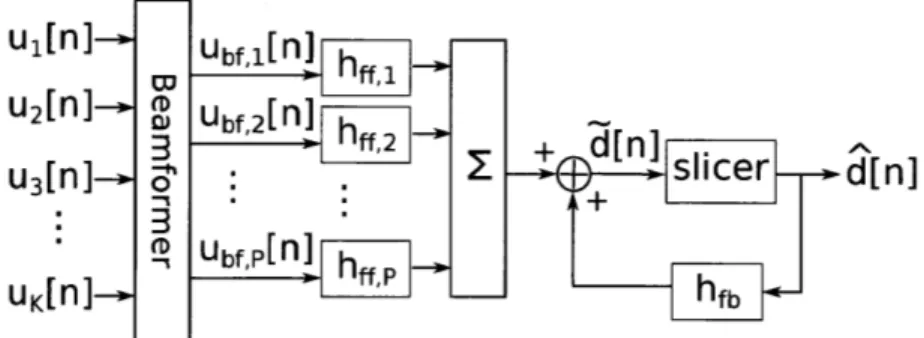
4.2.1 A multichannel decision feedback equalizer . . . . 78 4.2.2 A multichannel decision feedback equalizer with a beamformer

front-end to reduce computational complexity... . ... 80 4.3.1 Illustration of multipath and the physically constrained angle of arrival

for the shallow water communications channel. The angle of arrival of a path from the surface is defined to as 0 = 00, from the bottom 0 = 1800, and broadside 0 = 900. . . . . 83 4.3.2 Estimated angle of arrival and delay of the channel impulse response

arrivals from the from the SPACE08 experiment from Julian day 297 at time 1800. The white crosses indicate the arrival points calculated from the geometrical arrival model. The arrivals are labeled according to their interaction with the surface and bottom from the transmitter to the receiver: S indicates a surface bounce and B a bottom bounce. 84

4.4.1 First 5 DPSS coefficients for the DPSS with 24 coefficients constrained within a normalized bandwidth bounded by ±0.12. . . . . 90 4.5.1 Uniform weighted beampattern in k space at the design frequency of

the array. Note that the peak of beam is at the null of the adjacent b eam s. . . . . 91

4.5.2 Arrivals from SPACE08 data during calm weather conditions. The orange line specifies the delay calculated for the time-aligned uniform beam weights. Figure (a) shows the bounds for ab = 1 and figure (b)

with ab =

}..

4.5.3 Interconnections in adaptive beamformer-DFE algorithm, which could lead to possible instabilities... . . . . . . . ... 101

4.5.4 Hybrid-method for combining non-adaptive beamformer with adaptive beamformer. First the data is beamformed using a non-adaptive beam-former, such as a set of DPSS beams or uniformly weighted beams, and then the signal is sent through an equalizer and beamformer which are allowed to adapt to the signal. . . . . 102

4.6.1 Estimate of a time-varying channel impulse response. The data is from the SPACE08 experiment, with a 1000 m propagation distance from transmitter to receiver and a RLS channel estimator is used. The color scale indicates the magnitude of the channel estimate in time and delay. This figure illustrates that the channel delay spread is simple to

approximate, but the number of multipath arrivals is not apparent. . 104

4.7.1 Setup of SPACE08 experiment... . . . . . ... 121

4.7.2 Comparison of beamforming methods using SPACE08 experimental data. The left column ((a), (c), and (e)) contains the beamspace and adaptive methods. The right column ((b), (d), and (f)) contains the non-adaptive methods. (a) and (b) are results using data taken on day 297, time 1800, calm conditions. (c) and (d) are results using data taken on day 294, time- 1200, smooth, rolling waves. (e) and (f) are results using data taken on day 300, time 0800, very stormy conditions. 124

4.7.3 Results from SPACE08 comparing the beamspace, adaptive, non-adaptive, and hybrid methods for three sea surface conditions: (a) calm [day 297, time 1800] (b) rolling waves [day 294, time 1200] and (c) [day 300, time 0800]. In all three cases, the relative performance of the beamspace processing is reduced as the SNR is reduced. For the other methods the performance is approximately equivalent with the adaptive meth-ods having the best performance as the sea surface conditions become rougher. ... ... ... ... .. 125

4.7.4 Procedure for estimating the subspace dimension from data. . . . . . 127

4.7.5 Number of arrival estimation for data gathered on day 297, time 1800 at the SPACE08 experiment. All results presented use 500, 000 signal sample, with 6 samples per transmitted symbol. Four different meth-ods are presented: AIC is the Akaike information criterion, BIC is the Bayesian Information Criterion, DoF is the generalized x2 _method

us-ing the correlation matrix, and DoFMM is generalized x2 _{the method of}

moments. Different averaging windows are used: (a) length 50 averag-ing window, (b) length 100 averagaverag-ing window, (c) length 500 averagaverag-ing window, and (d) length 1000 averaging window. samples is used and in (b) an averaging window of 1000 samples is used. There was an overlap length of half the averaging window. The solid black line shows the carrier frequency and the dash-dot lines show the transmitted signal bandwidth... . . . . . ... 129

4.7.6 Comparison of mean squared error verses the number of beams for (a) DPSS beamformer and (b) Fully Adaptive beamformer. The black dashed line is the number of arrivals estimated by the ray-path model. 130

4.7.7 Comparison of beamforming methods using MACE10 experimental data. The left column ((a), and (c)) contains the beamspace and adaptive methods. The right column ((b) and (d)) contains the non-adaptive methods. The two rows represent different data sets, taken two minutes. The first column was taken at time 1810, and the sec-ond at time 1812. Note that the adaptive methods have a significant, relative loss of performance at low SNR... . . ... 132 4.7.8 Results from MACE10 comparing the beamspace, adaptive, non-adaptive,

and hybrid methods for two different data packets: (a) at time 1810 (b) at time 1812. Both of these results show the relative performance degradation of the adaptive results compared with the non-adaptive re-sults. This is due to the instabilities in the adaptive algorithm forcing the use of longer averaging windows. . . . . 133 4.7.9 Results from MACE10 comparing MSE for the data set from time

1812 at an SNR of 10dB with A = 0.996. (a) shows the adaptive and beamspace results, (b) shows the non-adaptive methods, and (c) compares the two. Notice that all of the adaptive methods have a point where the algorithm becomes unstable and the estimates are no longer valid . . . . 134

5.4.1 (a) BER and (b) MSE comparison of different LE approaches for a sim-ulated 7-coefficient stationary channel. The approaches include DA, CE error-estimated (Preisig [75]), CEB bias compensated, CEB regu-larized (Lee and Cox [58]), and optimal where perfect channel knowl-edge is assumed (no channel length estimation error). . . . . 152 5.4.2 (a) BER and (b) MSE comparison of different DFE approaches for

a simulated 7-coefficient stationary channel. The approaches include DA, CE error-estimated (Preisig [75]), CEB bias compensated, CEB regularized (Lee and Cox [58]), and optimal where perfect channel knowledge is assumed (no channel length estimation error). . . . . 153

5.4.3 (a) BER and (b) MSE comparison of different DFE approaches for a simulated 7-coefficient Rayleigh channel. The approaches include DA, CE error-estimated (Preisig), CEB bias compensated, CEB regular-ized (Lee and Cox), and optimal where perfect channel knowledge is assumed (no channel length estimation error). . . . . 154 5.5.1 Channel estimate for the observed data packet. Fairly calm conditions

with little channel spread. . . . . 157 5.5.2 (a) BER and (b) MSE comparison of different DFE equalizer

ap-proaches. The three approaches included are DA, CEB bias compen-sated, and the CEB error estimated proposed by Preisig [75]. The approach proposed by Lee et al. [58] is not included because the previ-ous results showed that it was not an optimal approach, i. e. the average error increased with SNR... . . . . . . 158 6.2.1 Correlation function for Markov channel model with a' = 0.99 and

o i = 0.0199. . . . . 162 6.2.2 Correlation function for Gaussian channel model with o, 1 and

=.. 164

6.7.1 The correlation of a single-coefficient Markov channel with a correlation window of Njin = 2400 symbols. There is a smooth transition from the channel correlation down to a minimum correlation as the SNR increases. ... ... ... ... .. 191 6.7.2 The correlation of a single-coefficient Gaussian channel with a

correla-tion window of Nwin = 2400 symbols. There is still a smooth transition from the channel correlation down to a minimum correlation as the SNR increases, with a slightly different shape than the AR(1) channel. 192 6.7.3 Realization of the 10-coefficient WSSUS, AR(1) channel where all

co-efficients have equal variance. The sum of the average energy of all the channel coefficients is unity. The color indicates intensity on a linear scale. . . . 193

6.7.4 Realization of the MMSE feedforward DFE coefficients for the channel shown in figure 6.7.3 with no noise. Notice that the first coefficient dominates over the others for all time. The color corresponds to mag-nitude and the scale is 20logO(h)... . . . ... 194 6.7.5 Correlation between the first coefficient of the equalizer and the inverse

of the first coefficient of the channel. There is a strong linear correlation between the two. There is also many non-correlated events indicating the approximation is not perfect.. . . . . . . . . 195 6.7.6 Correlation function for the first coefficient of the channel and the first

coefficient of the equalizer for several SNR values. Notice that there is a smooth transition from the correlation of the channel down to the 90dB. This trend continues as the SNR continues to be increased (not shown). The transition to the no-noise correlation levels happens at much higher SNR than for the single coefficient channel (shown in the figure at 200dB ). . . . . 196 6.7.7 Comparison of the CEB and DA algorithms using a 10-coefficient

Acronyms

Acronym Definition AoA Angle of Arrival

BPSK Binary Phase Shift Keyed CEB Channel Estimate Based

DA Direct Adaptation

DFE Decision Feedback Equalizer

EW-RLS Exponential-Weighted Recursive Least-Squares FSK Frequency Shift Keyed

IID Independent and Identically Distributed ISI Inter Symbol Interference

MAE Minimum Achievable Energy MCM Multiple Constraint Method MMSE Minimum Mean Squared Error MSE Mean Squared Error

MVDR Minimum Variance Distorionless Response PSD Power Spectral Density

PSK Phase Shift Keyed

QAM Quadrature Amplitude Modulation QPSK Quadrature Phase Shift Keyed

continued from last page.. . Acronym Definition

RF Radio Frequency

RLS Recursive Least Squares SDE Soft Decision Error

SINR Signal-to-Interference-plus-Noise Ratio SNR Signal-to-Noise Ratio

SOFAR Sound Fixing And Ranging

Chapter 1

Introduction

Since the dawn of time, people have looked at the surface of the ocean and wondered what secrets might be hidden in the depths. Born out of this wonder, oceanography is a science devoted to understanding the mysteries of the seas. Oceanographers have made many important discoveries that have fundamentally changed our understand-ing of the world. Technology is a drivunderstand-ing force behind many of these underwater discoveries. One important part of technology, and not coincidentally the focus of this thesis, is wireless communication. In oceanography, wireless communication is used to increase portability, simplify deployments, and decrease mission cost.

Acoustic radiation is currently the only practical way to wirelessly transmit in-formation underwater distances more than a few hundred meters. Wideband electro-magnetic radiation is common in terrestrial communications but is highly attenuated after propagating short distances through the ocean: electromagnetic radiation in the megahertz to gigahertz range (radio frequency or RF radiation) propagates only a few meters before being attenuated and electromagnetic radiation in the optical range (es-pecially blue-green light) propagates around a hundred meters. In contrast, acoustic radiation has relatively low attenuation and can propagate long distances through the ocean. Acoustics have been used to signal through thousands of kilometers of water [129] and have been used in virtually every ocean environment

[77].

The goal of wireless, acoustic communication is to transmit digital data reli-ably with minimum data rate and maximum power constraints. There are several

challenges when communicating acoustically through the underwater channel: inter-symbol interference (ISI) caused by reverberation [76], limited signal bandwidth due to frequency dependent absorption [103], and time-variability of the channel [75]. Every ocean environment (i.e. every communication setup) has unique operating pa-rameters (depth, system geometry, water column chemistry, etc.) so there is no uni-versal underwater acoustic channel model for system analysis. As a result, underwater communication systems are often adaptively tuned based on in-situ measurements.

To mitigate channel induced signal distortions, the received signal is filtered in a structure known as an equalizer. An equalizer produces an estimate of the transmitted symbol using a weighted combination of the received signal and, in some structures, past symbol estimates. The metric used to gauge equalizer performance is the average squared error between the equalizer output and the transmitted data symbol.

Adaptive equalizers were initially designed for the wired telephone channel [62, 63] using several simplifying assumptions, such as slow time-variation and white observa-tion noise. These approximaobserva-tions do not generally hold for the underwater acoustic channel; new thinking is needed to design equalizers that handle the harsh condi-tions of the underwater channel (e.g. large delay-spread, quickly varying coefficients, frequency selective fading, etc.) and that are computationally simple enough to be implemented on real-time systems. Using physical understanding of the underwater acoustic communication channel this thesis proposes several equalizer improvements with particular attention toward limiting computational complexity.

1.1

Contributions of this thesis

The goal of this thesis is to analyze past equalizer design assumptions and propose new algorithms for limiting complexity and improving performance. Specific contributions toward this goal are:

1. A description of how the physical considerations of the communication channel affect the structure of the effective noise correlation matrix used in the compu-tation of the equalizer coefficients.

The effective noise includes observation noise, sensor noise, and noise from chan-nel estimation errors. Traditionally, the effective noise correlation matrix has been approximated using a scaled identity matrix. Chapter 3 shows that the mean squared error can be reduced by as much as 4 dB using a fully pop-ulated effective noise correlation matrix and the computational complexity is reduced by assuming a Toeplitz matrix structure (which also further reduces mean squared error).

2. Analysis showing the best non-adaptive combination of elements from a multi-element receiver that reduces computational complexity without sacrificing per-formance.

In Chapter 4, a set of static beams is found which reduce computational com-plexity without sacrificing too much performance (at most a decibel or two degradation in performance). Experimental data reveals that there are some channel conditions, such as calm seas with a low signal-to-noise ratio where the non-adaptive beams outperform a fully-adaptive beamspace processor. Data-driven techniques for determining the appropriate number of beams are ana-lyzed.

3. An analysis of how fixing the channel model order affects the mean squared error equalizer performance.

A channel estimate based equalizer requires a fixed number of modeled channel coefficients. In Chapter 5 it is shown that when the model has a different number of coefficients than the true channel, equalizer performance is degraded. A method of improving performance by adjusting the noise correlation matrix is detailed.

4. A comparison of direct adaptation and channel estimate based equalizer algo-rithms, showing why the channel estimate based has lower mean squared error at high SNR.

have lower mean squared error than estimates from direct adaptation equaliz-ers. Chapter 6 presents new analysis which explains this effect; (MMSE) equal-izer coefficients have a shorter correlation window than channel coefficients, so tracking the equalizer coefficients (i.e. DA equalization) has higher mean squared error than tracking the channel coefficients (channel estimate based equalization).

1.2

Related work

This thesis focuses on analysis of the decision feedback equalizer (DFE) for underwater communication. There are many references which discuss the operation of the DFE in a variety of contexts, such as [79, 86]. Monsen [64] wrote a seminal paper examining the effect of DFE equalization on a fading channel where theoretical lower performance bounds were derived. Qureshi [81] wrote a nice tutorial paper summarizing the work on adaptive equalization prior to 1985.

The goal of most equalizers is to reduce the squared error between the data symbol estimate and the true data symbol. There have been several studies examining the nature of this error. Eletheriou and Falconer [31] examined how recursive least squares (RLS) tracking error affected DFE performance. They proposed separating the error into the sum of two parts: one term caused by channel estimation errors due to time variability and another term caused by noise.

Stojanovic [106] proposed an alternate decomposition of the error term: first into causal and a-causal parts and then into a channel estimation error part and a noise part. She postulated if the channel estimation error could be estimated, it could be combined with the observation noise estimate to create a total (effective) noise estimate. She and Zvonar extended this research into multi-user equalization in [111].

One form of the MMSE equation for equalizer coefficients is an inverse matrix multiplied by a column vector. Dzung [27] simplified equalizer error analysis of adap-tive algorithms by replacing the inverse of the random matrix with the inverse of the expectation of the random matrix.

Preisig [75] examined how imperfect channel estimation affected the equalizer taps. He proposed an estimated error DFE, where the error covariance matrix is estimated using the received signal, past data symbols, and a channel estimate. His work showed definitively that the effective error can be modelled as the noise plus a term which accounts for channel estimation errors.

Building on the work of Eleftheriou and Falconer [31], Nadakuditi and Preisig

[65,

Stojanovic et al. pioneered the analysis and application of advanced equalization techniques for the underwater communication [80, 105, 107, 108, 110]. Using ex-perimental data, she verified that equalization was possible underwater. She also examined some environmental factors that affect communication, such as noise and absorption, and derived useful approximations [101, 103].

Preisig et al. also how ocean physics affects underwater communication systems in [74, 75, 76, 78]. They focused on the effect of time-varying environments (surface waves) on communication systems and how to compensate for environmental distor-tions using equalization. One interesting observation was that waves act as a concave mirrors which focuses the acoustic energy and causes large, fast amplitude changes at the receiver. Li et al. [60, 59] proposed using the delay-Doppler characterization of the channel along with sparse techniques to mitigate this effect of these mirrors.

In a seminal work on multichannel, adaptive equalization for underwater com-munication, Stojanovic et al. [105] found that the optimal multichannel combiner is a matched filter followed by a maximum likelihood sequence estimator (MLSE). Since the MLSE is impractical due to the large channel delay spread in underwater environments (which can span hundreds of symbols), she used an adaptive DFE as the channel combiner. Using experimental data, she showed that for the underwater

channel, the mean squared error of the multichannel DFE output is not significantly greater than the mean squared error of the MLSE output.

The same set of authors showed that when the direction of arrival for all multipath components is known a multichannel DFE with a beamformer is equivalent to a multichannel DFE without a beamformer [109]. They further showed that any set of beam-weights that spans the signal space produces equivalent mean squared error performance when the observation noise is spatially and temporally white. Using the multichannel DFE with a beamformer reduced the computational complexity of the receiver when the number of multipath arrivals was less than the number of sensors.

Using physics-based constraints, the communication receiver can better estimate the channel and reduce computational complexity by reducing the number of param-eters to be estimated. Kraay and Baggeroer [50] proposed using physical constraints for array processing by constraining the signal covariance matrix to be realizable when the received signal was a sum of narrowband plane waves. Their goal was to reduce the number of snapshots needed to properly estimate a covariance matrix.

Papp et al. [71, 72] used a different form of physical constraint: mode-filtering. They showed that mode-filtering improves array signal-processing. They also showed using experimental data that mode-filtering a signal before equalization had higher mean squared error than an equalizer with no mode-filter.

LeBlanc and Beaujean [55, 56] proposed applying principle component analysis (PCA) to acoustic communication systems with receive arrays. To improve equalizer performance the beams were decorrelating by using the eigenvectors of the received signal correlation matrix were used as the beamformer weights. They focused mainly on the decorrelating effects of this technique and not on dimensionality reduction.

Two common methods for computing adaptive equalizer coefficients are direct adaptation (DA) where the equalizer coefficients are estimated directly from the re-ceived data and channel estimate based (CEB) where a channel estimate is used to compute the coefficients. There have been several studies comparing the DA equal-ization with CEB equalequal-ization, but the performance comparisons contained only em-pirical evidence without analysis. Many authors had hypotheses about the cause of

the performance difference, but there was no consistency between them.

An often cited work comparing DA and CEB equalizers on a Rayleigh fading channel is by Shukla et al. [91]. The authors showed that when the channel order is known and the signal to noise ratio (SNR) is large, the DA approach had higher mean squared error than the CEB approach.

Fechtel and Meyr [32] also demonstrated a difference in mean squared error (at high SNR) between DA and CEB equalizers, assuming the CEB equalizer had perfect channel knowledge. They hypothesized that the difference was due to the lag in the DA equalizer which implicitly has to estimate the channel state information.

Lee and Cox [58] examined the performance difference between the DA and CEB methods when the the true channel order was not known. They experimentally validated that for an unknown channel length the DA method outperformed the CEB method. They also found that a matrix regularization term was effective to combat the difference in performance between the two methods. In later work [57] examined the effect of channel mismatch on the bit error rate (BER) of a maximum likelihood sequence estimator (MLSE).

An alternative to equalization is time-reversal [33, 85]. In time-reversal techniques, a channel estimate is convolved with the data signal. The channel is estimated by sending a pulse through the channel and recording the received signal. This form of channel estimation is not robust to channel variations. An array is used to either transmitted or receive (or both) which provides an array gain proportional to the number of sensors in the array. Time-reversal methods both temporally and spatially match filter the received signal to increase the effective SNR.

Time-reversal has been shown to be an effective, low-complexity method for han-dling the difficulties of the underwater channel [46, 47, 85] and has been extended into multi-user scenarios [95, 96, 97]. Results have been confirmed using experimental data [28, 40]. After comparing the mean squared error of time-reversal with equal-ization, the equalizer always had lower mean squared error [128]. An equalizer is thus generally preferred to time-reversal. Attempts have been made to include both time-reversal and equalization into one communication system [17, 18, 98].

There has been increasing interest in combining equalization with error correcting coding, a technique known as turbo-equalization [26, 49, 117, 118]. The data is first encoded using an error correcting code and the resulting signal is transmitted through a channel. The equalizer filters the received signal and, rather than making a symbol decision, transmits the filtered output directly to the decoder. The raw output of the equalizer without a symbol decision is known as soft information. A decoder uses this soft information to refine the transmitted symbol probabilities. The updated soft information is sent back to the equalizer and the process iterates.

Turbo-equalization has been shown to work well for underwater channel [19, 20, 25, 92]. One issue with turbo-equalization is its computational complexity. There has been work done to reduce the computational complexity [93, 117], but still more needed. The techniques presented in this thesis could be applied to the equalizer portion of a turbo-equalizer to improve performance and reduce computational com-plexity in underwater environments.

1.3

Organization

The remainder of this thesis is organized as follows: Chapter 2 provides the mathemat-ical and conceptual background to understand the remainder of the thesis. Chapter 3 describes how channel estimation errors can be accounted for when calculating equal-izer filter weights. Chapter 4 explains how knowledge of the physically constrained arrival angles can be incorporated into an array receiver to reduce computational complexity. Chapter 5 presents analysis of how assumptions of the channel order affect the equalizer error. Chapter 6 discusses the difference between the CEB and the DA equalizers. Concluding remarks and areas for future research are identified in Chapter 7.

1.4

Notation

Throughout this thesis, the following notation is used:

Symbol Definition

a Non-bold lowercase letters represent scalar constants a Bold lowercase letters represent column vectors A Bold uppercase letters represent matrices

* Complex conjugate of the variable (i.e. a*)

T _{Transpose of a vector or matrix (i.e.}

AT)

H _{Hermitian (conjugate transpose) of a vector or matrix (i.e. AH)} - 2-norm of the enclosed quantity (i.e. ||a||)

^ Estimate of a quantity (i.e. i)

I Square Identity matrix (context sized) IM MxM Square Identity Matrix

0 Zero matrix or vector (context sized) E{-} Expectation of enclosed quantity

Chapter 2

Background

2.1

Underwater communication

The underwater channel remains one of the most challenging communication environ-ments. Designing a reliable communication system remains an active area of research. Knowing where a system is going to be deployed is important when designing under-water acoustic (UWA) communication system. Communicating vertically through the ocean tends to be the simplest regime since often there is little multipath. The name of this environment is the Reliable Acoustic Path (RAP) [24] due to the fidelity of the channel. Baffles or directional hydrophones are used reduce effects of surface bounces.

In deep water systems there is less interaction with the surface so the communica-tion channel is time-invariant, possibly sparse, and widely spread in delay. Modeling techniques are often employed in deep water channels to determine the locations where communication is possible due to the channel physics. The direct path is often the last to arrive in deep water since a natural waveguide exists around the sound-speed minimum in deep water [42].

In shallow water environments interactions with the time-varying ocean surface are unavoidable. There are also interactions with the bottom and nearby obstacles plus noise from waves, shipping traffic, and marine life. When operating in such a dynamic environment adaptive channel tracking and adaptive equalization techniques

are essential, such as the exponentially weighted recursive least squares (EW-RLS) algorithm.

Underwater communication began with the uncoded, analog underwater telephone or "the Gertrude" which was used to commzunicate with a manned submersible. As higher data-rates became necessary and the intended receiver was a machine instead of a person more complex systems were needed. The development of these systems began in the analog domain, but quickly switched to the digital domain where frequency shift keying (FSK) and more recently phase shift keying (PSK) (for increased bandwidth efficiency) are used for data modulation. Many detailed papers have been written concerning the history of underwater communications such as [5, 14, 15, 16, 45, 1101. The focus of this thesis is on the well-mixed, shallow-water channel where the isovelocity assumption is appropriate. Data is modulated using phase shift keying (PSK) techniques since this is the current state of the art. The following subsections outline some of the difficulties in communicating through the underwater environment to familiarize the reader and to emphasize that this is a harsh environment that requires extra effort.

2.1.1

Distance and SNR

The majority of ocean noise can be separated into one of four components: turbulence, shipping, wind, and thermal noise. Turbulence dominates in the low frequency region under 10 Hz, shipping noise is dominant in the 10-100 Hz region, wind-driven wave noise prevails in the 100 Hz -100 kHz, and thermal noise dominates above 100 kHz [102]. The total noise is the unweighted sum of these four noise components. A useful approximation of the noise power spectral density (PSD) as a function of the frequency

f

10 logia N(f) ~ Ni - logio f. (2.1.1) The above expression has units dB re pPa per Hz and the constants are Ni = 50 and

- 18 [102].

driven noise is dominant. With some notable exceptions (e.g. snapping shrimp and breaking ice), noise in the acoustic communication frequencies is well modeled by a Gaussian random process [102, 126]. In general, the power spectral density of this process is not flat, so the noise process is not white.

Attenuation is a function of the acoustic path length I and the frequency of the

signal

f

[10, 103]

A(l,

f)

where k is the spreading factor (cylindrical, spherical, etc.), a(f) is the absorption coefficient, and 1_{, is a reference distance. Thorp [115, 116] provided an approximate}

expression for the absorption coefficient as a function of frequency which is valid for frequencies in the range 500 Hz to 50 kHz. Most acoustic communication frequencies are in this range. The expression for the absorption coefficient is

10 log a(f) = 0.11 + 44 +2 2.75. 104 f2 _{+ 0.003, (2.1.3)} 1 + f 2 _{4100 + f}2

where the quantity 10 log a(f) has units of dB/km and

f

f

10 logo a(f) = 0.11 2 + 0.011f 2 + 0.002 (2.1.4)

1

is a better approximation [10, 102]. Fisher and Simmons [34] tied these expressions to physical and chemical properties of sea water.

Using a narrowband approximation and ignoring any multi-path effects, the SNR can be approximated as a function of frequency and distance,

SNR(l,

f)

P/A(

P

N(f)Af A(l, f)N(f)A(f)'

where Af is the bandwidth of the receiver and hence the received noise (narrow-band approximation) [102]. The frequency dependent portion of this expression is

20 Distance 50 km -140--150- Distance= 100 km - -160--- 170 0 2 4 6 8 10 12 14 16 18 20 Frequency [kHz]

Figure 2.1.1: Signal to Noise ratio (narrowband), 1/A(l,f)N(f), as a function of fre-quency for various ranges.

encompassed in the expression A(1, f)N(f) since P is the total source power across the available bandwidth. Using a practical spreading coefficient of k = 1.5, Figure 2.1.1 shows the relationship between frequency and SNR, recreated from [102]; both the optimal center frequency and 3 dB bandwidth are dependent on transmission range.

Jensen and Kuperman [41] performed a related analysis to find the optimum fre-quency that balanced the propagation and attenuation mechanisms of the shallow water channel, but did not account for noise power. The optimum frequency is a general feature of waveguide or ducting propagation and for shallow water channels is strongly dependent on depth [42]. Typical optimum frequencies when the water depth is 100 m are 200-800 Hz, lower than the frequencies found in [102] which included the noise characterization.

2.1.2

Delay spread of the channel

As sound travels from the transmitter to the receiver, it follows not only a direct path, but also additional paths due to reflections from the surface, reflections from the sea floor, and inhomogeneities in the sound speed profile which cause the refraction of the sound paths.

The time difference between the first received path and the last is referred to as the delay-spread of the channel. The delay-spread determines the fastest rate at which data can be transmitted without inter-symbol interference (ISI). Often the length of the delay-spread is in units of transmitted symbol durations, the inverse of the transmitted symbol rate. Delay spreads of tens and hundreds of symbols are not uncommon in the underwater channel. This is a stark contrast to the radio-frequency

(RF) channel which often has on the order of three symbols of ISI.

The delay-spread of the underwater communications channel is due to the different paths from the transmitter to receiver. In water shallow enough for an approximately isovelocity sound speed profile the delay spread induced by the channel is due to reflections from the sea surface, reflections from the bottom, and reflections from anything in the water column. These reflections are referred to as macro-multipath since they are due to macro features in the environment. These features are usually assumed to be roughly time-invariant over a time-scale that is much larger than the data signaling rate [100].

The acoustic rays are better modeled as three-dimensional tubes rather than two-dimensional lines. When the tube encounters an object, the reflections are usually not point reflections, but are reflections from an area such as a rough patch of sand or rough sea surface. This causes each ray path to spread in time, sometimes by as much as a few milliseconds. The multipath due to small scale features such as surface roughness and random ocean fluctuations is referred to as micro-multipath. Micro-multipath is non-specular and some components of the small scale random fluctuations can be modeled statistically [100]. In the acoustics literature, the micro-multipath concept is also known as ray-tubes [42].

Figure 2.1.2: Diagram depicting some of the acoustic paths from the transmitter to the receiver. The black solid lines show the path and the blue cylinder are an example of the spreading in space that would cause a spread in time at the receiver.

Figure 2.1.2 shows an example of what multipath might look like in a shallow water environment. The macro-multipath is represented by the different paths (solid black lines) and the micro-multipath is a cylinder around this line, indicating the spreading radius.

In a deep water environment, in addition to surface and (less commonly) bottom bounces, fully refracted paths occur due to a local minimum in the sound speed profile. Sound tends to "favor" regions with slower sound speed and will bend towards those regions. There is a region of the ocean known as the Sound Fixing and Ranging (SOFAR) channel or the deep sound channel where the sound speed is at a minimum. The ray bending is due to Snell's law applied to a medium with a continuously changing sound speed. The deep water channel can have a large time-spread but may be sparse and is often slowly-varying compared to the time scales of equalizer

adaptation relevant for acoustic communication.

Regions of little acoustic penetration due to system geometry and the sound speed profile are known as shadow zones. These regions can occur because of obstructions (e.g. sea mounts) or more importantly because of the waveguide propagation physics. Shadow zones can form in either the deep or shallow water channels [42, 119]. There is little signal processing that can be done to correct for shadow zones so compensation for shadow zones is accomplished through system placement and mission design.

2.1.3

Doppler, waves, and motion

Each of the transmitter-to-receiver paths experience varying degrees of time-variability effects due to surface waves, internal waves, platform motion, reflections from moving objects, and currents and tides. Each source of variability can induce either a Doppler shift, where all of the frequencies are shifted up or down, or a Doppler spread, where neighboring frequencies are smeared together. A typical Doppler spread is on the or-der of 0 to 30 Hz, but depends heavily on the transmit frequency and communication system parameters (sea surface motion, weather, platform motion, etc.).

Because the speed of sound is much slower than the speed of light, the Doppler effects observed in the underwater channel tend to be much more severe than in RF channels. To illustrate the Doppler effect more clearly, consider a pulse, p(t), modulated with a carrier frequency of

fc

rO - 2, where To is a reference delay. The Doppler effect is proportional to a = v/c8.

The transmitted signal, s(t), is [104]

s(t) = Re{p(t)e2 fct}. (2.1.6)

The signal observed by the receiver is

[104]

r(t) = s(t + - To) = s(t + at - To) = Re{p(t + at - To)eJ2

fetat--)} (2.1.7)

CS

With respect to the center frequency the baseband receive signal (i.e. the received signal after demodulation and low pass filtering) is [104]

f

p(t(1 + a)). A dilation the time domain causes a corresponding contraction of the frequency response.

2. The signal has a frequency offset of afc, which is known as a Doppler shift.

The dilation effect can be ignored when the time-bandwidth of the signal is appro-priately small. If the bandwidth of p(t) is denoted as Bp, the signal is approximately time invariant for a time B-1. If the data packet has total duration T, then the total dilation of the packet is vT/cs which must be much less than B-1 _{for dilation to be}

ignored. Therefore, when the time bandwidth product, TB,, satisfies the relation

T B, < cS V

dilation can be ignored; otherwise, the received signal needs to be re-sampled [120]. Another way to characterize the Doppler is through the scattering function. As-sume that the channel coefficient at a particular time t and delay T is g(t, 7). If the

channel is known to be wide sense stationary (i.e. the correlation is a function of the time difference), then the temporal correlation function of the channel is

R₉(At; T₁, T₂) = E{g(t, Tl)g* (t + At, T2)}, (2.1.9)

which is a function of three variables: the two delays, T and T2, and the difference in

time At. The scattering function of the channel is defined as the Fourier transform of the temporal correlation function,

Sg(Ad; T1, T2)= J Rg(At; i, T ₂)e-j 2 AdtdAt, (2.1.10)

where Ad is the Doppler spreading variable. At a particular delay, T1 = 72, this is

an expression of the Doppler spread of the channel. This leads to the relationship between the coherence time of the channel, (At)c, and the Doppler spread, Bd, [79]

The coherence time, (At)c, i.e. the time over which the channel at a particular delay is correlated, is approximately the inverse of the Doppler spread of the channel, Bd.

For time-invariant channel (At)c = oc, so there is no Doppler spread.

In addition to Doppler effects, there are other channel effects caused by the waves. For certain geometries, the waves will act as a concave mirror and the focus the acoustic energy to cause severe but brief changes in the channel magnitude and phase characteristics [78, 74]. These focusing events cause the path that interacts with the surface to have a larger magnitude than the direct path and can cause instantaneous ir/4 shifts in phase.

Wave motion can also inject bubbles into the water volume [77]. These create a highly variable medium for the sound to propagate through and can increase the absorption coefficient or reduce the effective height of the water column.

2.2

Channel model

An underwater communication systems consists of at least one transmitter and one receiver. Figure 2.2.1 shows an example setup for an underwater acoustic experiment.

~1-100 M

~ 0.1-100 km

Figure 2.2.1: Possible setup for acoustic model being studied in this thesis.

Received signals are assumed to be sampled at baseband, so the analysis and processing are done in discrete time with complex valued signals. The acoustic channel is modeled with a finite extent, linear, time-varying impulse response plus additive

noise [79, 120]. The received signal sample at time n, u[n), can be written as [75]

Nc-1

u[n] =

g*[n,

k]d[n - k] + v[n),

(2.2.1)

k=-Na

where d[n] is the transmitted data, v[n] is complex, baseband noise, and g[n, k] is the complex, baseband channel impulse response equating the input data at time n - k to the output data at time n. The channel includes the transmit and receive filtering effects in addition to the physical propagation effects. The channel is assumed to have Nc causal coefficients and Na acausal coefficients, where the center (zero offset) coefficient is assumed to correspond to the center of the direct arrival. This definition is particular to the isovelocity channel; in other environments the direct arrival may not be the first causal arrival (e.g. the direct arrival is the last arrival for the SOFAR channel). Eq. (2.2.1) can be written more compactly as

u[n] =g[n d'[n] + in], (2.2.2)

with

g[n] = [g[n, Nc - 1] ... g[n, 0] ... g[n, -Na]]T (2.23)

and

d'[n] = [d[n - Ne + 1] ... d[n] ... d[n + Na]]T. (2.2.4)

Stacking successive received signal samples, eq. (2.2.2) becomes a matrix-vector equa-tion,

u[n] = GH [n]dj[n] + v[n], (2.2.5) where u[n] is a vector of sampled received data, d[n] is the transmitted data, v[n] is

the sampled noise vector, and G[n] is the channel convolution matrix. Specifically,

u[n] = [u[n - Le +1] ... u[n] ... u[n+ La] ]T (2.2.6)

d[n] = [d[n - L- N +

2]

where La and Lc are the number of acausal and causal feedforward equalizer taps in each feedforward section of a decision feedback equalizer. The transmitted data symbols are assumed to be drawn from a zero-mean random-process with variance o-. The noise and transmitted data correlation matrices are defined as

R, E{v[nivHnl} (2.2.10)

Rd A E{d[n]dH[ }j = o~21 = I. (2.2.11)

The last equality for Rd highlights an assumption used for the remainder of this thesis (unless otherwise noted) that the transmitted data symbols are white with

unit energy, i.e. or-= 1.

Each of the columns of the matrix G[n], denoted above as g'[m], is the channel impulse response vector at time m, g[m], padded with zeros so the matrix multiplica-tion GH [nd[n] is equivalent to the convolumultiplica-tion of the channel impulse response with the transmitted data from eq. (2.2.1).

To handle fractionally spaced sampling (more than one sample per symbol), the number of rows of G[n] is increased proportional to the fractional sampling rate (number of samples per symbol). The length of the noise and received data vec-tors is increased accordingly. The length of the transmitted symbol vector remains

unchanged. Except when noted, symbol rate sampling is assumed for notational sim-plicity; it is straightforward to extend the results to handle fractional-rate sample spacing.

2.3

Least-squares estimation

2.3.1

Setup

Many problems from signal processing, communications, and control have a similar form: estimate the vector w when the statistics of the random vector x and random variable y are known, v is random noise, and

y = w HX + V1

Since the noise is random it is not possible to estimate w exactly so a metric is needed to determine the quality of the estimate. An extremely common metric is the mean squared error metric which is the expected absolute difference squared between y and

Yest = wH x where West is the estimate of w. The minimization problem using this

metric is

WMMSE = arg min E{ y - w(2.3.1)

West

The solution to this minimization problem is the minimum mean squared error (MMSE) solution

WMMSE

=

where R, = E{xxH} x,r = E{xy*}, and P R- 1. Assuming both x and y are zero-mean, this solution provides the unbiased estimate of the parameter vector w with the minimum mean squared error. The solution can be modified to handle the non-zero mean case as well. In the communication context, the MMSE problem setup is used for channel estimation and for equalizer coefficient estimation.