Applying sampling and predicate pushdown in an interactive data exploration system

Applying Sampling and Predicate Pushdown in an

Interactive Data Exploration System

by

Jason Lam

Submitted to the

Department of Electrical Engineering and Computer Science

in partial fulfillment of the requirements for the degree of

Master of Engineering in Electrical Engineering and Computer Science

at the

MASSACHUSETTS INSTITUTE OF TECHNOLOGY

May 2020

© Massachusetts Institute of Technology 2020. All rights reserved.

Author . . . .

Department of Electrical Engineering and Computer Science

May 12, 2020

Certified by. . . .

Tim Kraska

Associate Professor, Thesis Supervisor

Accepted by . . . .

Katrina LaCurts

Chairman, Master of Engineering Thesis Committee

Applying Sampling and Predicate Pushdown in an Interactive

Data Exploration System

by

Jason Lam

Submitted to the

Department of Electrical Engineering and Computer Science on May 12, 2020, in partial fulfillment of the

requirements for the degree of

Master of Engineering in Electrical Engineering and Computer Science

Abstract

Interactive data exploration (IDE) systems require low latency and high performance, as users expect to see their ad-hoc queries return results quickly for a seamless expe-rience. Predicate pushdown is a common performance optimization for systems that rely on databases, by pushing the filtering that was originally performed by the over-arching system down to its underlying database systems. In this work, we implement both sampling and predicate pushdown in Northstar, a system for interactive data science. We then investigate and benchmark optimization strategies for predicate pushdown in Northstar, and find that a cache-aware "adaptive" pushdown strategy leads in the greatest performance gain in many cases.

Thesis Supervisor: Tim Kraska Title: Associate Professor

Acknowledgments

A couple words of appreciation for those who have helped me throughout my under-graduate years and on my thesis, and helped me reach the point where I am today:

• I would like to thank Professor Kraska for his support and guidance through my masters program, and for his great teaching of 6.814, which deepened my understanding of databases and motivated me to reach out for a UROP. • Thank you to Zeyuan Shang and Emanuel Zgraggen for their constant support

and valuable insight during our weekly meetings that helped shape this work. • Thank you to my family for providing emotional support, and also for feeding

me while I was stuck at home due to COVID-19.

• Thanks to my friends, for making my MIT experience unforgettable—in particular, thanks to Ashley, Joanna, Kevin, and Daniel, for being weebs, despite me not being one.

Contents

1 Introduction 11 2 Related Work 17 3 Background 19 3.1 Overview . . . 19 3.2 Davos Context . . . 19 3.2.1 Planner . . . 20 3.2.2 Sample Manager . . . 21 3.2.3 Stream Manager . . . 22 3.2.4 Scheduler . . . 22 3.3 Example . . . 22 4 Implementation 25 4.1 Predicate Pushdown . . . 25 4.1.1 Query Transformation . . . 26 4.1.2 Cache-Awareness . . . 28 4.2 Sampling Pushdown . . . 29 4.3 Configuration . . . 29 4.4 Testing . . . 29 5 Results 31 5.1 Datasets . . . 31 5.2 Experiments . . . 31

6 Conclusion 37

List of Tables

5.1 Small DB Runtimes (s) by Predicate Selectivity . . . 32 5.2 Large DB Runtimes (s) by Predicate Selectivity . . . 33 5.3 Small DB Fully In-Cache (s) Runtimes by Predicate Selectivity . . . . 34 5.4 Large DB Fully In-Cache Runtimes (s) by Predicate Selectivity . . . . 35 A.1 Schema for Large and Small DBs . . . 39

Chapter 1

Introduction

Data science has become more and more important in our increasingly digitized world, and making data science more accessible has also become more important as a re-sult. That is the aim of Northstar, an interactive data science system that aims to democratize data science by simplifying its use for domain experts who may not be trained in statistics or computer science [8]. The system was inspired by scenes in ac-tion movies where computer operators interact with data visually using touch or pen interfaces. Those characters are not typing up SQL queries or manually constructing charts; their user interfaces allow for data in charts and tables to be interacted with directly. In a similar vein, Northstar is a system designed for interactive whiteboards, where manually typing up queries is infeasible.

Why were interactive whiteboards chosen as the target platform? For starters, hologram technology is not quite mature yet, so perfectly replicating the action movie scenes is not an option. These interactive whiteboards are the next best thing, since they are essentially large TVs that support multi-touch input, and are already used in classrooms and meeting rooms as a collaboration tool. Northstar hopes to make the scenario where domain experts and data scientists work together during a meeting and achieve fast results a reality, which is in contrast with the current state of things are where they require several meetings to establish a starting point, from which the data scientist will refine offline.

a tool like Northstar. One glaringly obvious problem is how text-based these systems are. The SQL queries used as inputs are strings, and the output rows are strings as well. One reason why interactive whiteboards are so conducive to collaboration is that they provide a big enough screen to keep everyone on the same page, but this advantage diminishes when all the inputs and outputs are text-based. Northstar aims to fix that by having an intuitive GUI [3] where users can automatically see graphs and charts of their data without having to build them manually. Users can drag and drop UI elements to construct new SQL queries, and the outputs of the queries are presented visually [2].

Figure 1-1: Screenshot of Northstar’s GUI in action [12]

However, just having a nice GUI for existing DBMSs is not enough to be an effective interactive data science (IDE) system. Consider a tool that was just a pretty wrapper around a DBMS, but included no additional features. Domain experts would not be able to use it to do data science right away: a major problem that remains is that the overall system will be too slow. A recent study [10] found that delays of over 500ms can negatively impact the user’s experience, and a delay of one second is often used as an upper bound in human-computer interaction literature for how long you can keep the user waiting before they lose their train of thought. A typical query

on DBMS with a large amount of data can take on the order of seconds or minutes, which is unacceptable for an interactive system where the user expects immediate feedback from their ad hoc queries.

One solution to this performance requirement is approximate query processing (AQP) [6]. AQP allows the system to return low-error approximate results with little delay, which achieves the interactivity necessary for a smooth user experience. While the user is looking at the approximate results, which are often accurate enough to draw early hypotheses on the data, the system can continue doing the full computation in the background, so that the initial result can eventually be refined into the full result. Another problem with DBMSs is that their queries are stateless and return batch results. A typical workflow on an interactive data exploration (IDE) system is con-structed incrementally, as the user "builds" up a query by dragging UI elements around and can see intermediate results every step of the way. Recreating this ex-perience with solely a DBMS would require waiting on a query to finish running whenever any UI element was moved, diminishing the interactivity aspect. Northstar circumvents this by having a robust cache; if a newly created query is just a re-finement of a previous query, we can immediately refine the previous query’s cached result instead of executing a new SQL query on the DBMS. While DBMSs can also make use of caches, DBMS caches were not designed for the use case of incremental queries, so their effectiveness in this scenario is much lower than Northstar’s caching solution.

In addition to the previous features, Northstar also features a virtual data scientist (VDS) component, which applies automated machine learning (AutoML), a technique that simplifies the process of using machine learning so that non-data scientists can apply machine learning models to their data. Users can apply machine learning models onto their data the same way they would apply any other operator. This allows domain experts to apply machine learning models to their data without having to learn how to use another tool.

While existing DBMSs may be inadequate to be used directly as IDE systems, Northstar’s purpose is not to replace existing data management stacks. Rather,

Northstar is designed to interoperate with existing infrastructure seamlessly, and does not store any data on its own. Instead, the data stays on the existing data storage infrastructure, and Northstar only requests streams from the existing infras-tructure to build up its in-memory sample to run queries. Therefore, users deciding to use Northstar would not be switching from their existing DBMSs to Northstar, but instead be adding Northstar to the top of their data management stack.

This interoperability allows for further optimizations, as there may be tasks that the data sources are faster at performing than Northstar. In this thesis, we explore an additional performance optimization that was not yet been implemented in Northstar: predicate pushdown. The concept of pushdown is quite simple: we can consider a case where Northstar is reading customer data from an Oracle database, and then filtering for all the entries where the age field is at least 30. Without predicate pushdown, Northstar would have to retrieve all the rows from an Oracle database using the query

SELECT * FROM customers;

and then do the filtering on its own. We can instead push the (age >= 30) predicate onto the database itself, so that the Oracle database is doing the filtering with the query

SELECT * FROM customers WHERE (age >= 30);

This approach leverages Oracle’s highly-optimized index on the predicate, and also results in fewer rows retrieved by Northstar. Therefore, the overall runtime of the system is improved. Note that what we pushed down in this example was a simple filter predicate supported by the underlying database; we would not be able to push down something like a machine learning model operator since it has no SQL support. Furthermore, we explore how to improve our predicate pushdown strategy by taking advantage of Northstar’s cache. Continuing from the previous example, if we were interested in refining the query to only look for users between the ages of 30 and 40, predicate pushdown would result in this query

to be executed on the underlying Oracle database. However, in this case we do not need to query the database at all; we already have the set of users over age 30 in our cache, so we can refine the existing cached data to avoid extraneous SQL queries.

To confirm that these optimizations are effective, we present a set of microbench-marks that test different systems and predicate selectivities and draw promising con-clusions from their results.

Along with predicate pushdown, we also explored sampling pushdown. While sampling pushdown is less well-known when compared to predicate pushdown, the two work very similarly. For example, Northstar can retrieve all of the rows from the same query

SELECT * FROM customers WHERE (age >= 30);

and proceed to sample 5% of the rows that were retrieved. The sampling could instead be pushed into the query, so that the query becomes

SELECT * FROM customers WHERE (age >= 30) SAMPLE(5);

and we avoid having to retrieve all the rows when what we wanted was just a random sample of 5% of them.

Chapter 2

Related Work

Predicate pushdown is not a recent idea. The concept of moving around predicates around for performance reasons has been explored as early as 1999 [9]. Predicate pushdown is available nowadays in a wide variety of systems that use an underly-ing database system, includunderly-ing large federated systems [11] and Data Stream Man-agement Systems [7]. Results from predicate pushdown have been very promising; Apache Spark has been benchmarked [1] to show significant speedups due to predi-cate pushdown, especially when the predipredi-cate being pushed down is highly selective. Therefore, the main priority of the project was to implementing robust pushdown predicate support in Northstar. However, blindly applying predicate pushdown may be ineffective; one test with the SQL Server feature PolyBase [5] showed a query that originally took 14.1 seconds without predicate pushdown taking 21 seconds after using predicate pushdown. To account for this, we also explore "smarter" strategies for applying predicate pushdown.

On the other hand, there is little existing literature on sampling pushdown. This may stem from the fact that many of the existing systems that leverage predicate pushdown were not designed to do any sampling on their own, and any sampling was already done by the underlying database, so there was never any opportunity for sampling pushdown.

Chapter 3

Background

3.1

Overview

Northstar is an interactive data science system designed with the goal of democ-ratizing data science, designed to be used with interactive whiteboards. As a web application, it can be accessed from any browser, and includes both a frontend and a backend application. In this thesis we focus on the Davos C++ backend system for Northstar, where the predicate and sampling pushdown occur.

Davos can be divided into three parts, as shown by Figure 3.1. The Davos interface allows the frontend client to make requests and receive data, the Davos Context manages the data samples and coordinates how the queries are performed, while the Davos workers actually execute the queries scheduled by the Davos Context. We discuss the Davos Context in further detail in the next section, as it is the part most relevant to predicate and sampling pushdown.

3.2

Davos Context

The Davos context manages all work to be done in the backend. It is composed of several different modules, but we will only cover the ones directly related to query processing.

Figure 3-1: Diagram of Davos’s architecture

3.2.1

Planner

This component converts job descriptions into jobs. It essentially translates logical query plans to their physical query plan equivalents, and we can modify this compo-nent to apply predicate or sampling pushdown during the translation. We go further in depth on the changes that were made to the planner component to implement pushdown in the next chapter.

Job Description

Job descriptions are logical query plans in Davos. They contain a set of data sources and steps, along with the sampling strategy for the data sources. It can be represented as a directed graph where each vertex is either a data source or a step, and each edge

points from a data source or step whose output stream is being used into the step that uses the output stream as one of its inputs.

Data Source

The data source objects represent any external data source. This includes, but is not limited to, SQL databases and CSV files. For SQL database data sources, the object records the information necessary to connect to and log into the database, along with a SQL query to actually retrieve a set of rows from said database.

Step

The step objects represent logical operations that Davos performs on the data re-trieved from its data sources. We are primarily interested in the filter step, which cover the predicates we are interested in pushing down, but there are other step types such as projections or joins.

Jobs

Jobs are physical query plans in Davos, and can be executed by the Davos workers. They contain information very similar to the job descriptions, but no longer include logical operators in the form of steps. Instead, they describe how to physically imple-ment the logical operations. Jobs are also optimized by the planner to not impleimple-ment extraneous steps whose output is unneeded for the final result.

3.2.2

Sample Manager

This component accesses external data sources to create data samples. If the under-lying data source is small enough, no sampling is done at all; instead, the entire data source is stored in the cache. Otherwise, reservoir sampling is performed to create a sample.

3.2.3

Stream Manager

This component converts the data read from external data sources into data streams with the Apache Arrow format. These data streams can be later cached or serialized to disk.

3.2.4

Scheduler

This component schedules jobs to be executed by the Davos workers. It can prioritize jobs in a variety of different strategies, such as weighing shorter jobs over longer jobs, or preferring jobs that further from completion over jobs that are almost finished.

3.3

Example

Suppose a user opens up Northstar in their browser, and asks to pull up the customer data set from an Oracle database.

First, the frontend client relays this web request to the Davos interface, which translates this request into a format that the Davos context can understand.

The job description for this request is simple; it consists of one data source and zero steps. The singular data source includes the SQL query

SELECT * FROM customers;

along with all the credentials necessary to actually connect to the Oracle database. The planner takes this job description and converts it into a job, where it is then passed onto the scheduler. Since there are no other jobs waiting, the job can be executed immediately, and it is transferred to an available Davos worker.

During the Davos worker’s execution, it finds that it needs to read from an Oracle database. The specific details are sent to the sample manager, which handles the specifics of connecting to the database.

The SQL query is finally executed on the Oracle database, and the results are received by the sample manager. Since this job doesn’t have any additional steps, the Davos worker does not need to do anything with the returned data stream, so the

data stream is returned through the Davos interface to be presented in a user friendly manner on the frontend client.

The user can see this newly displayed data and decide to look more deeply into the cohort of customers living in Massachusetts. After the request is sent from the frontend and received by the Davos interface, we now have a job description with one data source and one step. Ignoring the possibility of predicate pushdown in this example, the data source will still have the same SQL query

SELECT * FROM customers;

while new filter step stores the predicate

state = 'MA'

The planner takes this new job description, converts it into a job, and the scheduler decides when the job should be ran. The Davos worker in charge of executing this job will ask the sample manager to read the same data from the same Oracle database, since the new job’s data source is identical to the previous job’s data source. If that data is still in the cache, the stream manager will return the cached results; otherwise, it will go back and query the Oracle database again.

After the data stream is ready, the Davos worker goes through it and applies the

state = 'MA' filter. These filtered results are finally returned through the Davos interface, and the user can again look at these results to come up with new queries.

Chapter 4

Implementation

4.1

Predicate Pushdown

Applying predicate pushdown can be represented as a transformation from one query plan to another. By designing our predicate pushdown as a function that read in a logical query plan as an input and returned a logical query plan as an output, we could insert this right before the logical query plan was converted to a physical query plan. This way, predicate pushdown would be available for all executed queries, as each logical query plan must be translated to a physical query plan before execution. For the predicate pushdown function itself, we designed a greedy algorithm that would apply predicate pushdown to the first eligible filter it could find. An eligible filter satisfies the following requirements:

• The filter has only one input.

• The only input is a data source, and not another step.

• The input data source is a SQL database that supports predicate pushdown. After finding an eligible filter, its predicate is pushed down onto its data source, so a new data source is created that combines the old data source and the pushed down predicate. The filter can now be removed from the logical query plan, and steps that originally used that filter as an input are updated to use the new data source as an

input instead. However, the old data source cannot be removed, since there may exist other steps that still read from the original database.

We can repeat the previous process until there are no more filters that can be pushed down. Once no more eligible filters remain, we proceed with a final cleanup phase, where unused data sources are deleted. This involves going through the list of remaining steps, building up a set of used data sources, and then deleting the data sources not in the set. Since removing elements from the list shifts the IDs of the remaining data sources, each step has to updated afterwards to reflect the new position of its input data source.

4.1.1

Query Transformation

When we combine filters and data sources to create new pushed down data sources, we need new combined SQL queries for them too. However, the original data source’s SQL query could look like anything, and trying to insert a predicate into an arbitrary SQL query is very error-prone. For example, adding the predicate (age >= 30) into the following three SQL queries

SELECT * FROM customers ORDER BY age;

SELECT * FROM customers WHERE age <= 50 ORDER BY age;

SELECT * FROM customers where name = "WHERE"; should result in the following queries:

SELECT * FROM customers WHERE (age >= 30) ORDER BY age;

SELECT * FROM customers WHERE age <= 50 AND (age >= 30) ORDER BY age;

SELECT * FROM customers where name = "WHERE" AND (age >= 30);

Given the wide variety of different ways that the predicate could be inserted, manual string manipulation was out of the question. Another possibility would be to construct a syntax tree based on the original query, add the new predicate into the tree, and finally convert the new syntax tree into a SQL query. We couldn’t find any existing libraries that would simplify the conversion from syntax tree to SQL query string,

since databases that would be using such libraries only need the syntax tree to execute on, and reconstructing a SQL query string from the tree would be useless.

Therefore, we turned to instead using the original query as an inner query, so that the three example queries would become this instead:

SELECT * FROM

(SELECT * FROM customers ORDER BY age)

WHERE (age >= 30);

SELECT * FROM

(SELECT * FROM customers WHERE age <= 50 ORDER BY age)

WHERE (age >= 30);

SELECT * FROM

(FROM customers WHERE age <= 50 AND (age >= 30) ORDER BY age)

WHERE (age >= 30);

This nested query syntax was supported in every database we tried, from SQLite to Oracle.

The thing to watch out with this approach is having multiple layers of nesting, so that pushing down a second predicates into the same data source would not result in an additional layer of nesting. If we push down both (age >= 30) and (age <= 40) into the same data source with the original query SELECT * FROM customers, we would prefer

SELECT * FROM

(SELECT * FROM customers)

WHERE (age >= 30) AND (age <= 40); over

SELECT * FROM

(SELECT * FROM

(SELECT * FROM customers)

WHERE (age >= 30))

To achieve this, we can keep a record of which data sources have already been created through predicate pushdown while doing the pushdown. If we are creating a new data source from another data source that was created from pushdown, we simply need to add the new predicate at the end, so predicate pushdown adds at most one level of nesting no matter how many times a data source goes through predicate pushdown.

4.1.2

Cache-Awareness

The previous process converts a logical query plan to a simpler logical query plan with fewer steps, by performing predicate pushdown whenever it is possible. This is generally preferable, since there will be fewer rows retrieved from the database. However, in an IDE system where data sources can be cached, this can be suboptimal. Consider the scenario where a user first requests to see the set of customers that live in Massachusetts, and then further refines that query to get customers that live in Massachusetts over the age of 30.

By using the strategy of pushing down every predicate, our system has to make two separate database queries:

SELECT * FROM customers WHERE (state = 'MA');

SELECT * FROM customers WHERE (state = 'MA') AND (age >= 30); This strategy ignores the fact that we may already have the results from the first query in our cache, and it is often faster to just reuse those results with the new predicate than to start anew with a different database query.

We can improve the previous algorithm by adding a single additional requirement for filters to be eligible for pushdown: we now also skip applying pushdown to data sources that are already in the cache.

This new predicate pushdown algorithm runs exactly the same as the previous one when the cache is empty, but takes advantage of the cache when it is available. This was named the "adaptive" strategy, and was benchmarked against the "always pushdown" strategy in the next chapter.

4.2

Sampling Pushdown

Implementing sampling pushdown was very similar to implementing predicate push-down. The only main difference is that sampling syntax varies wildly between dif-ferent SQL databases. For example, Oracle offers a function for sampling, SAMPLE, while SQLite and MySQL have different functions for generating random numbers (RANDOM() and RAND(), respectively). Therefore, support for sampling was added individually for different databases.

4.3

Configuration

We added configuration settings for debugging and benchmarking purposes. The options for predicate_pushdown_strategy were:

• "always"- applies as much predicate pushdown as possible, ignoring the cache • "adaptive" - applies predicate pushdown while considering the cache

• "never"- does not apply predicate pushdown The options for sampling_pushdown_strategy were:

• "always" - apply sampling pushdown • "never"- do not apply sampling pushdown

4.4

Testing

To ensure correctness, unit tests were written to cover a wide variety of cases using a couple of different databases. We used the Googletest C++ framework to confirm that queries returned the same set of rows regardless of if pushdown was enabled or not.

Chapter 5

Results

5.1

Datasets

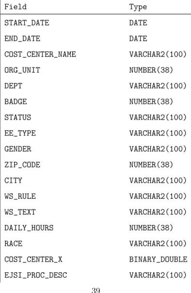
We use two Oracle databases to benchmark and evaluate our predicate pushdown im-plementation. The smaller database had about 30,000 rows, while the large database had 21 million. Since we wanted to experiment with predicates of different se-lectivities, we added sampler columns onto each database which stored a random value between 1 and 100. Then, the predicate that has a selectivity of 10% is just (sampler <= 10), while a predicate with a selectivity of 50% would be (sampler <= 50). Since our experiments involved logical query plans with two predicates, we added two of these sampler columns onto both databases. Now, we can combine a 50% selec-tivity predicate on the first sampler column and a 10% selecselec-tivity predicate on the second sampler column to get 5% of the overall rows, but still be able to benchmark the scenario where we only push down one of the predicates. The resulting table schema has been included in the Appendix as table A.1.

5.2

Experiments

We tested the adaptive predicate pushdown strategy against the always strategy on the same set of logical query plans. For the benchmark, we first warmed up the cache for the adaptive strategy by executing query plans with one predicate from

the first sampler column. The selectivities we chose for testing were 1%, 2%, 5%, 10%, 25%, and 50%. Then, we would construct the query plans for benchmarking by combining a predicate on the first sampler column with a predicate on the second sampler column. We tested every combination of query plans, and each is one cell in tables 5.1 and 5.2.

While sophisticated benchmarks for testing IDE systems do exist (for example, IDEBench [4]), we opted to use the simpler method of counting how many seconds each microbenchmark took to run. We decided that this method would be just as effective since we were trying to reduce query times in every scenario.

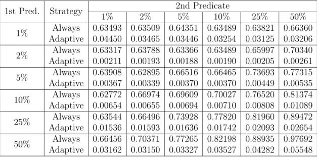
Table 5.1: Small DB Runtimes (s) by Predicate Selectivity

1st Pred. Strategy _{1% 2%} 2nd Predicate_{5% 10% 25% 50%} 1% _{Adaptive 0.04450 0.03465 0.03446 0.03254 0.03125 0.03206}Always 0.63493 0.63509 0.64351 0.63489 0.63821 0.66360 2% _{Adaptive 0.00211 0.00193 0.00188 0.00190 0.00205 0.00261}Always 0.63317 0.63788 0.63366 0.63489 0.65997 0.70340 5% _{Adaptive 0.00367 0.00339 0.00370 0.00370 0.00449 0.00535}Always 0.63908 0.62895 0.66516 0.66465 0.73693 0.77315 10% _{Adaptive 0.00654 0.00655 0.00694 0.00710 0.00808 0.01089}Always 0.62772 0.66974 0.69609 0.70027 0.76520 0.81374 25% _{Adaptive 0.01536 0.01593 0.01636 0.01742 0.02093 0.02654}Always 0.63544 0.66496 0.73928 0.77820 0.81960 0.89472 50% _{Adaptive 0.03162 0.03150 0.03327 0.03527 0.04282 0.05548}Always 0.66456 0.70371 0.77265 0.82198 0.88935 0.97692

From the results of table 5.1, we can see that the adaptive strategy outperforms the always strategy in every logical query plan when the database we’re querying from has a relatively small number of rows. Each query for the always strategy took between 0.6 seconds and 1 second to finish, while the adaptive strategy’s longest runtime was only 0.056 seconds.

Moving on to table 5.2, we can see that the adaptive strategy outperforms the always strategy in most logical query plans, and only underperforms when the com-bined predicates are very selective, but the cached predicate is not. In particular, we

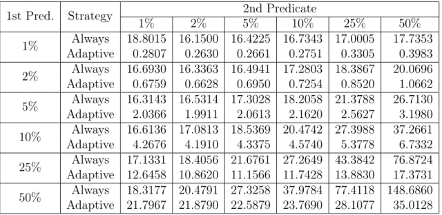
Table 5.2: Large DB Runtimes (s) by Predicate Selectivity

1st Pred. Strategy _{1% 2%} 2nd Predicate_{5% 10% 25% 50%} 1% _AdaptiveAlways 18.8015 16.1500 16.4225 16.7343 17.0005_{0.2807 0.2630 0.2661 0.2751 0.3305} 17.7353_0.3983 2% _AdaptiveAlways 16.6930 16.3363 16.4941 17.2803 18.3867_{0.6759 0.6628 0.6950 0.7254 0.8520} 20.0696_1.0662 5% _AdaptiveAlways 16.3143 16.5314 17.3028 18.2058 21.3788_{2.0366 1.9911 2.0613 2.1620 2.5627} 26.7130_3.1980 10% _AdaptiveAlways 16.6136 17.0813 18.5369 20.4742 27.3988_{4.2676 4.1910 4.3375 4.5740 5.3778} 37.2661_6.7332 25% _{Adaptive 12.6458 10.8620 11.1566 11.7428 13.8830}Always 17.1331 18.4056 21.6761 27.2649 43.3842 76.8724_17.3731 50% _{Adaptive 21.7967 21.8790 22.5879 23.7690 28.1077}Always 18.3177 20.4791 27.3258 37.9784 77.4118 148.6860_35.0128

can see that when the cached predicate has a low selectivity of 50% but the other predicate has a high selectivity of either 1% or 2%, the always strategy manages to execute slightly faster.

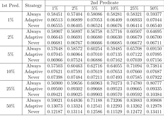
We then tried to compare both the adaptive pushdown strategy and the always pushdown strategy against the never pushdown strategy, and the results from the smaller database are presented in table 5.3.

We can see that applying pushdown is actually a huge performance decrease when the entire database is already in the cache, which is a logical extension of the previous idea that using reusing something that already exists in the cache is generally going to be better than issuing a new database request. The always pushdown strategy takes between 0.5 and 0.9 seconds for each query, while the adaptive pushdown and never pushdown strategies take between 0.06 to 0.14 seconds, varying based on the number of returned rows.

These results also assure us that adopting the adaptive pushdown strategy over the never pushdown strategy (the status quo) only adds a negligible performance hit, if any, since the difference between any adaptive pushdown and never push-down runtime is 0.01 seconds at most. This minimal overhead is due to the extra

Table 5.3: Small DB Fully In-Cache (s) Runtimes by Predicate Selectivity 1st Pred. Strategy _{1% 2%} 2nd Predicate_{5% 10% 25% 50%}

1% Adaptive 0.06513 0.06899 0.07053 0.06409 0.06933 0.07044Always 0.58451 0.57404 0.58086 0.58281 0.58321 0.59377 Never 0.06555 0.06405 0.06524 0.06676 0.06414 0.06540 2% Adaptive 0.06643 0.06691 0.06680 0.06630 0.06679 0.06700Always 0.58907 0.56897 0.56758 0.57716 0.60507 0.64695 Never 0.06681 0.06767 0.06666 0.06685 0.06672 0.06711 5% Adaptive 0.07045 0.06964 0.07010 0.07135 0.07122 0.07095Always 0.57648 0.58572 0.60254 0.59485 0.65708 0.69150 Never 0.06966 0.07524 0.06886 0.07162 0.07039 0.07156 10% Adaptive 0.07621 0.07591 0.07619 0.07653 0.07660 0.07687Always 0.57503 0.60463 0.62716 0.64055 0.71094 0.73814 Never 0.07398 0.07484 0.07211 0.07493 0.07585 0.07922 25% Adaptive 0.09500 0.09302 0.09668 0.09523 0.09665 0.09335Always 0.56900 0.59656 0.66963 0.70273 0.74780 0.80777 Never 0.09421 0.09025 0.09903 0.09570 0.09592 0.10384 50% Adaptive 0.13073 0.13324 0.12541 0.12293 0.13262 0.12978Always 0.59021 0.64836 0.71188 0.73206 0.83883 0.89808 Never 0.12187 0.13114 0.12586 0.11529 0.12472 0.13411

computation necessary to check if pushdown is necessary; in the never pushdown strategy, the code path that checks the cache is entirely skipped.

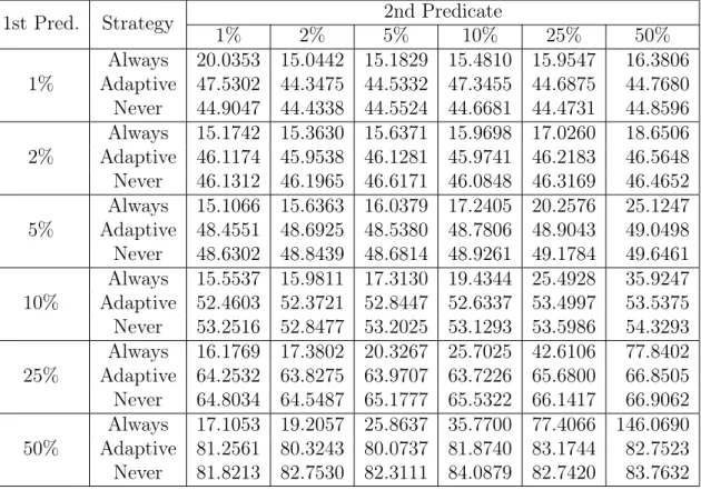
The strategy of always using the cached results instead of apply pushdown does show its weaknesses when applied to the larger database, as shown in table 5.4.

Here, we see that the adaptive pushdown strategy continues to use the cached database, even though the entire underlying database does not fit in the cache. This means that the adaptive pushdown strategy mirrors the never pushdown strategy when the full database has been cached, disregarding the possibility where using the cached version is slower than requerying the database for a smaller result first. In the large database case, the fact that the DBMS is faster at filtering the data more than offsets the extra network calls Northstar has to make. This disparity in efficiency may be due to differences in how the data is represented and scanned through in Oracle, and could also be attributed to the fact that Northstar and the Oracle database are

Table 5.4: Large DB Fully In-Cache Runtimes (s) by Predicate Selectivity 1st Pred. Strategy _{1% 2%} 2nd Predicate_{5% 10% 25% 50%}

1% Adaptive 47.5302 44.3475 44.5332 47.3455 44.6875Always 20.0353 15.0442 15.1829 15.4810 15.9547 16.380644.7680 Never 44.9047 44.4338 44.5524 44.6681 44.4731 44.8596 2% Adaptive 46.1174 45.9538 46.1281 45.9741 46.2183Always 15.1742 15.3630 15.6371 15.9698 17.0260 18.650646.5648 Never 46.1312 46.1965 46.6171 46.0848 46.3169 46.4652 5% Adaptive 48.4551 48.6925 48.5380 48.7806 48.9043Always 15.1066 15.6363 16.0379 17.2405 20.2576 25.124749.0498 Never 48.6302 48.8439 48.6814 48.9261 49.1784 49.6461 10% Adaptive 52.4603 52.3721 52.8447 52.6337 53.4997Always 15.5537 15.9811 17.3130 19.4344 25.4928 35.924753.5375 Never 53.2516 52.8477 53.2025 53.1293 53.5986 54.3293 25% Adaptive 64.2532 63.8275 63.9707 63.7226 65.6800Always 16.1769 17.3802 20.3267 25.7025 42.6106 77.840266.8505 Never 64.8034 64.5487 65.1777 65.5322 66.1417 66.9062 50% Adaptive 81.2561 80.3243 80.0737 81.8740 83.1744Always 17.1053 19.2057 25.8637 35.7700 77.4066 146.069082.7523 Never 81.8213 82.7530 82.3111 84.0879 82.7420 83.7632

running on separate machines with different specifications.

One may wonder how the adaptive strategy can get results closer to the always strategy in this scenario. We would need to use a more sophisticated strategy when deciding whether to use the cached results or not. In the smaller database case, the total number of rows cached in the first place was small, so we always want to use the cached results; in the larger database example, we usually do not. However, even with the larger database there is still a point where it becomes inefficient to create a new query. This is evident in the case where predicate selectivity is at its lowest; since the large database contains 21 million rows, filtering it with two filters with 50% selectivity returns 5.25 million rows, and it appears that when the returned result set is that large it becomes better to use the cached results. It seems like the most effective heuristic would be to estimate the size of the resulting query set and compare it with the size of the cached result set before deciding whether to use the

cached results or not, but designing and implementing such a heuristic is outside this thesis’s scope.

However, there is a simpler optimization that can help result in getting the results from 5.2 when using the adaptive pushdown strategy; if both the result set for the whole database and the result set for a single predicate are cached, we should use the more specific (and smaller) of the two cached results. This still requires the existing greedy pushdown algorithm to be refactored, and thus is also out of scope.

Chapter 6

Conclusion

In this thesis, we explored the benefits of implementing predicate and sampling push-down in the Northstar IDE system. We provided an overview of what Northstar aims to accomplish, and explain how the addition of pushdown supports that goal. We also cover the differences between Northstar and traditional DBMSs are, to provide context for why implementing predicate and sampling pushdown in Northstar is a unique problem. After describing what pushdown is and what it is effective for, we discuss more in-depth what the challenges of adding pushdown are, and cover how an adaptive cache-aware pushdown strategy can outperform a non-cache-aware strategy. After comparing the runtimes of both strategies, we find a substantial performance improvement when using the adaptive strategy in most scenarios.

Appendix A

Database Schema

Table A.1: Schema for Large and Small DBs

Field Type START_DATE DATE END_DATE DATE COST_CENTER_NAME VARCHAR2(100) ORG_UNIT NUMBER(38) DEPT VARCHAR2(100) BADGE NUMBER(38) STATUS VARCHAR2(100) EE_TYPE VARCHAR2(100) GENDER VARCHAR2(100) ZIP_CODE NUMBER(38) CITY VARCHAR2(100) WS_RULE VARCHAR2(100) WS_TEXT VARCHAR2(100) DAILY_HOURS NUMBER(38) RACE VARCHAR2(100) COST_CENTER_X BINARY_DOUBLE EJSI_PROC_DESC VARCHAR2(100)

EJSI_LINE_LOC VARCHAR2(100) COUNT_EJSI_SIGNINS NUMBER(38) HALL BINARY_DOUBLE TENURE_YRS BINARY_DOUBLE AGE_AT_HIRE BINARY_DOUBLE SHIFT VARCHAR2(100) START_DATE_MONTH VARCHAR2(100) JOIN_MONTH VARCHAR2(100) LABEL NUMBER(38) TRAIN_TEST VARCHAR2(100) AGE_CURRENT NUMBER(38) VOLUME BINARY_DOUBLE REPAIR_MINUTES BINARY_DOUBLE COUNT_NON_DP_VINS_HALL BINARY_DOUBLE RMU_HALL_MONTH BINARY_DOUBLE DPU_HALL_MONTH BINARY_DOUBLE F1_DP_HALL_MONTH BINARY_DOUBLE ATT_POINTS BINARY_DOUBLE HEADCOUNT_MAU_CC BINARY_DOUBLE HEADCOUNT_BMW_CC BINARY_DOUBLE TOTAL_HEADCOUNT_CC BINARY_DOUBLE COUNT_FEMALE_CC BINARY_DOUBLE COUNT_MALE_CC BINARY_DOUBLE COUNT_NOGENDER_CC BINARY_DOUBLE PERCENTAGE_FEMALE_CC BINARY_DOUBLE AVG_TENURE_CC BINARY_DOUBLE AVG_TENURE_BMW_CC BINARY_DOUBLE COUNT_BMW_EMPLOYEES_TENURE BINARY_DOUBLE AVG_TENURE_MAU_CC BINARY_DOUBLE COUNT_MAU_EMPLOYEES_TENURE BINARY_DOUBLE

COUNT_HIRED_MAU BINARY_DOUBLE COUNT_HIRED_BMW BINARY_DOUBLE COUNT_TERMIANTED_BMW BINARY_DOUBLE COUNT_TERMIANTED_MAU BINARY_DOUBLE LINE_LOC VARCHAR2(100) AVG_HOURS_AT_LINE_LOC BINARY_DOUBLE MAX_HOURS_AT_LINE_LOC BINARY_DOUBLE AVG_REG_HOURS BINARY_DOUBLE SUM_REG_HOURS BINARY_DOUBLE AVG_OT_HOURS BINARY_DOUBLE SUM_OT_HOURS BINARY_DOUBLE ENCRYPTED_BADGE VARCHAR2(100) SAMPLER NUMBER(38) SAMPLER_2 NUMBER(38)

Bibliography

[1] Boudewijn Braams. Predicate pushdown in Parquet and Apache Spark. Master’s thesis, Universiteit van Amsterdam, 2018.

[2] Andrew Crotty, Alex Galakatos, Emanuel Zgraggen, Carsten Binnig, and Tim Kraska. Vizdom: Interactive analytics through pen and touch. Proc. VLDB Endow., 8(12):2024–2027, August 2015.

[3] Andrew Crotty, Alex Galakatos, Emanuel Zgraggen, Carsten Binnig, and Tim Kraska. The case for interactive data exploration accelerators (IDEAs). In Proceedings of the Workshop on Human-In-the-Loop Data Analytics, HILDA ’16, New York, NY, USA, 2016. Association for Computing Machinery.

[4] Philipp Eichmann, Carsten Binnig, Tim Kraska, and Emanuel Zgraggen. Idebench: A benchmark for interactive data exploration, 2018.

[5] Kevin Feasel. PolyBase Revealed, chapter 4. Apress, Berkeley, CA, 2019.

[6] Alex Galakatos, Andrew Crotty, Emanuel Zgraggen, Carsten Binnig, and Tim Kraska. Revisiting reuse for approximate query processing. Proc. VLDB Endow., 10(10):1142–1153, June 2017.

[7] Lukasz Golab, Theodore Johnson, and Oliver Spatscheck. Prefilter: Predicate pushdown at streaming speeds. pages 29–37, 01 2008.

[8] Tim Kraska. Northstar: an interactive data science system. Proceedings of the VLDB Endowment, 11:2150–2164, 08 2018.

[9] Alon Levy, Inderpal Mumick, and Yehoshua Sagiv. Query optimization by pred-icate move-around. VLDB, 03 1999.

[10] Zhicheng Liu and Jeffrey Heer. The effects of interactive latency on exploratory visual analysis. Visualization and Computer Graphics, IEEE Transactions on, 20:2122–2131, 12 2014.

[11] Mary Roth and Laura Haas. Cost models do matter: Providing cost information for diverse data sources in a federated system. 10 1999.