Publisher’s version / Version de l'éditeur: Energy and Buildings, 2017-09-19
READ THESE TERMS AND CONDITIONS CAREFULLY BEFORE USING THIS WEBSITE. https://nrc-publications.canada.ca/eng/copyright
Vous avez des questions? Nous pouvons vous aider. Pour communiquer directement avec un auteur, consultez la première page de la revue dans laquelle son article a été publié afin de trouver ses coordonnées. Si vous n’arrivez pas à les repérer, communiquez avec nous à [email protected].
Questions? Contact the NRC Publications Archive team at
[email protected]. If you wish to email the authors directly, please see the first page of the publication for their contact information.
NRC Publications Archive
Archives des publications du CNRC
This publication could be one of several versions: author’s original, accepted manuscript or the publisher’s version. / La version de cette publication peut être l’une des suivantes : la version prépublication de l’auteur, la version acceptée du manuscrit ou la version de l’éditeur.
For the publisher’s version, please access the DOI link below./ Pour consulter la version de l’éditeur, utilisez le lien DOI ci-dessous.
https://doi.org/10.1016/j.enbuild.2017.09.048
Access and use of this website and the material on it are subject to the Terms and Conditions set forth at
Potential energy savings from high-resolution sensor controls for LED
lighting
Dikel, Erhan E.; Newsham, Guy R.; Xue, Henry; Valdés, Julio J.
https://publications-cnrc.canada.ca/fra/droits
L’accès à ce site Web et l’utilisation de son contenu sont assujettis aux conditions présentées dans le site LISEZ CES CONDITIONS ATTENTIVEMENT AVANT D’UTILISER CE SITE WEB.
NRC Publications Record / Notice d'Archives des publications de CNRC: https://nrc-publications.canada.ca/eng/view/object/?id=6729a7d5-ccc7-45e8-b6bf-34f5028c018f https://publications-cnrc.canada.ca/fra/voir/objet/?id=6729a7d5-ccc7-45e8-b6bf-34f5028c018f
Accepted Manuscript
Title: Potential Energy Savings from High-Resolution Sensor Controls for LED Lighting
Authors: Erhan E. Dikel, Guy R. Newsham, Henry Xue, Julio J. Vald´es
PII: S0378-7788(17)31639-0
DOI: http://dx.doi.org/10.1016/j.enbuild.2017.09.048 Reference: ENB 7967
To appear in: ENB
Received date: 8-5-2017 Revised date: 14-8-2017 Accepted date: 16-9-2017
Please cite this article as: Erhan E.Dikel, Guy R.Newsham, Henry Xue, Julio J.Vald´es, Potential Energy Savings from High-Resolution Sensor Controls for LED Lighting, Energy and Buildingshttp://dx.doi.org/10.1016/j.enbuild.2017.09.048
This is a PDF file of an unedited manuscript that has been accepted for publication. As a service to our customers we are providing this early version of the manuscript. The manuscript will undergo copyediting, typesetting, and review of the resulting proof before it is published in its final form. Please note that during the production process errors may be discovered which could affect the content, and all legal disclaimers that apply to the journal pertain.
Potential Energy Savings from High-Resolution
Sensor Controls for LED Lighting
Erhan E. Dikel*, Guy R. Newsham, Henry Xue, Julio J. Valdés
National Research Council Canada. 1200 Montreal Road, Building M-24, Ottawa, K1A 0R6, ON, Canada *Corresponding author. Tel.: +1 613 993 9625.
Highlights for the submission of the article: Potential Energy Savings from High-Resolution Sensor Controls for LED Lighting.
- Modelling and demonstrations were used in a full scale office test bed to illustrate the energy savings potential associated with a high-resolution sensor network combined with a spatially-defined and granular LED lighting system.
- Real occupancy data measured in real office environments were used to estimate a reduction in timeout period from the current code maximum of 20 minutes to 1 minute. - The potentials of energy savings were tested by adding daylight harvesting to the
high-resolution occupancy detection network. This combination resulted in 79% energy savings compared to typical prevailing energy code provisions for open-plan offices.
ABSTRACT
LED lighting systems paired with high-resolution sensor systems offer great potential for
substantial energy savings via enhanced control options, and have other value-added features. We used modelling and demonstrations in a full-scale office test bed to illustrate this potential. First, we propose that such a system enables much shorter timeout periods for occupancy sensing: the higher density of sensors provides more reliable occupancy detection and LEDs are impervious to lifetime degradation from the consequent increased switching frequency. We used occupancy data measured in real office environments to estimate that a reduction in timeout period from the current code maximum of 20 minutes to 1 minute would yield 26% additional energy savings. Further, we installed 72 LED luminaires in an office test bed with windows; each luminaire featured a co-located motion sensor and light sensor. The localized light sensor enabled daylight harvesting at each fixture to be optimized to local spatial
conditions, yielding an extra 35% energy savings compared to a single photosensor controlling all luminaires, and ensuring better delivery of target horizontal illuminance values across the space. Finally, we demonstrated a combination of local occupancy and daylight harvesting features that resulted in 79% energy savings compared to typical prevailing energy code provisions for open-plan offices.
2
Keywords: High-resolution sensors, Light-emitting diodes (LEDs), Energy efficiency, Occupancy sensing, Daylight harvesting
1. Introduction
Rising energy prices, changing building energy regulations and sustainability motivate
governments, utilities, building owners and end users to invest in and support effective energy saving strategies. Some existing commercial buildings are equipped with lighting control systems that facilitate certain energy management strategies such as daylight harvesting, occupancy-based controls, time scheduling, task tuning, personal controls and demand
response. Most new buildings in North America feature more than one of these strategies as a consequence of compliance with energy codes [ASHRAE, 2010; CCBFC, 2011], and pursuit of voluntary green building certification [Baylon & Storm, 2008]. The lighting industry and codes and standards bodies are united in seeking even greater energy savings through the
deployment of light-emitting diode (LED) technology. In addition to the higher efficacy offered by LEDs, they offer more control potential than fluorescent systems, and a platform for a greater density of environmental sensors, which may be leveraged for enhanced control options and other features.
Occupancy sensors and their energy saving potential with fluorescent lighting have been extensively studied. Williams et al. [2012] reviewed the literature and calculated the average energy savings due to various lighting controls identified in more than 80 papers. They reported that the average energy savings attributable to occupancy-based controls in real installations was around 24%. However, occupancy rates in a space directly affect the energy saving performance of such control systems. In office settings, savings in private offices tend to be relatively high, whereas in shared spaces savings may be lower as a single occupant of a larger space is all that is needed to keep the lights on.
The current energy efficiency codes for commercial buildings require a lighting control device for many space types (including private, but not open-plan, offices) that turns off the lights no later than 30 minutes after all occupants have left the space [ASHRAE, 2010; CCBFC, 2011]. This timeout interval is likely to be reduced to 20 minutes in future code iterations, and is most commonly achieved using a single motion sensor utilizing passive infra-red (PIR) technology installed on the ceiling or wall of a space. The timeout period recognises the inherent inaccuracy of a single PIR motion sensor at short time scales, [Newsham et al., 2015; Tiller et al., 2010] such that lights are only switched off after no motion is detected throughout the entire period. This reduces the potential for false negatives (control system concluding that the space is empty when it is not), which can be very annoying to the occupants.
It has long been recognised that substantial savings are possible with shorter timeout periods. For instance, Richman et al. [1996] calculated 23% savings (compared to no controls) from four offices with a 20-minute timeout, which increased to 76% savings when the timeout was
reduced to 2 minutes. There are many energy efficient LED luminaires on the market with built-in occupancy (and other) sensors as standard, offerbuilt-ing the potential of multiple sensors per space that may be leveraged. For example, Tiller et al. [2009, 2010] demonstrated that with a
3
greater number of sensors in a single space the accuracy of occupancy detection can be improved and timeout periods can be realistically shortened.
Nonetheless, for fluorescent lighting systems shorter timeouts might not be desirable because of the adverse effect of the increased number of switching cycles on lamp lifetime. Von Neida et al. [2001] calculated energy savings in private offices during work hours with timeout periods as short as five minutes. However, they noted that increased maintenance and lamp replacement costs would ensue. Cycling frequency is not a determining factor in LED life [USDoE, 2009], which opens the door for shorter switching periods where detection accuracy is sufficiently high. Similarly, the energy saving potential of daylight harvesting – dimming or switching electric lighting if daylight can contribute to some or all of a space’s lighting needs – has been estimated or measured in many studies. Williams et al. [2012] reported that the average energy savings attributable to daylight harvesting as measured in actual installations was approximately 28%. However, the savings in any given space depend on many factors, including window size, space geometry, building location, time of year, and interior finishes and geometry.
In an intelligent lighting control system, each luminaire can be provided with a photosensor in addition to an occupancy sensor. Instead of having a single photosensor controlling multiple rows of luminaires as a group as in conventional daylight harvesting, a photosensor may control its local luminaire individually. This will likely increase the energy saving potential and the system robustness.
The potential for such advanced control options on LED platforms has been recognized by other researchers in the field. Notably, Philips Research in the Netherlands has published several papers in which they proposed control algorithms to support some of these features [van de Meugheuvel et al., 2014; Caicedo et al., 2011; Pandharipande and Caicedo, 2011]. The focus of these papers has been on simulation of systems, with limited demonstration in hardware or on the system stability in delivering the desired illuminance levels. In this paper we model and demonstrate an enhanced lighting control system in an open-plan office setting and in a full-scale test bed, with a focus on the energy savings potential compared to conventional approaches.
The remainder of this paper is organized as follows: Section 2 describes calculations to determine the energy savings attributable to occupancy sensing systems with shorter timeout periods in an open-plan office context. Section 3 describes a full-scale open-plan office test bed in which advanced occupancy sensing and daylight harvesting systems were successfully demonstrated. These systems leveraged high-resolution information from sensors collocated with luminaires, and delivered substantial energy savings compared to existing practice. Section 4 provides some further discussion and observations, and potential additional applications for such a sensor network. Section 5 offers concluding remarks.
2. Modelling of Shorter Occupancy Timeouts
4
We based our model on the layout of the test bed utilized in our subsequent full-scale demonstrations (described in Section 3), although some details were not identical. The
modelled space was 12 m x 7 m x 2.7 m, with six cubicle workstations, each measuring 1.8 m x 2.4 m. The cubicles were centered in the space with a circulation area around the cluster of workstations. The surface reflectance of the floor, perimeter wall and ceiling were 20%, 50% and 80%, respectively, which is typical for lighting calculations [Illuminating Engineering Society of North America. 2013]. Each workstation had 1.5 m height partitions with a 30% reflectance; desk surfaces had a 50% reflectance.
We based our calculations on actual measured occupancy patterns in similar, real spaces. We chose two separate occupancy data sets to provide some diversity. The first set of occupancy data was obtained from a study conducted by Galasiu and Newsham [2009] in an office area with cubicle workstations featuring dimmable direct-indirect fluorescent luminaires with built-in PIR occupancy sensors, occupied by regular staff conducting normal office tasks. Occupancy data were recorded every five minutes from June 9th, 2006 to July 31st, 2007. The second
occupancy data set was collected in private and shared office spaces in various office buildings, at 15-second intervals over several months in 2013, using a pressure-sensitive floor mat to indicate occupancy [Newsham et al., 2015]. We selected the occupancy data collected in six offices in each data set from 10 non-contiguous days between 7:00 A.M. and 7:00 P.M. The choice of six offices matched the number of workstations in the modelled space, and 10 days provided a reasonable and manageable variety of occupancy patterns.
For the modelling exercise we used the same lighting system as in our full-scale test bed (Section 3), but configured slightly differently. Seventy-two LED spotlights were distributed over the ceiling of the space, on a 61 x 61 cm (2 x 2 ft.) grid in a rectangular layout over the
workstations only, so that each workstation had 12 dedicated LED luminaires. The LED
luminaires were dimmed to 81% of full output to provide an average light level on the desktop of approximately 350 lux at a lighting power density (LPD) of 13.5 W/m2 (calculated over the
footprint of the cubicles alone)1. Each LED luminaire had a co-located motion sensor to facilitate
very high accuracy occupancy detection, allowing for shorter timeout periods to be modelled with an expectation of reliability. We modelled several occupancy-based control scenarios, as described in Table 1.
2.2 Results
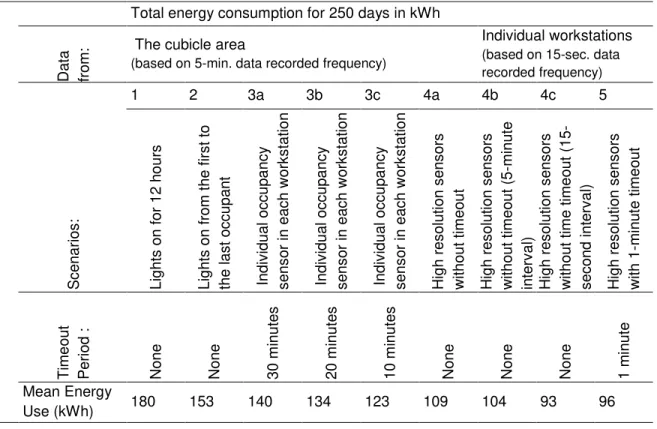
Table 2 shows the total calculated energy consumption of the various scenarios; values were calculated over 10 weekdays of collected occupancy data, and then extrapolated to 250 workdays to represent an annual estimate2.
3. Automatic Control Trials in an Open-Plan Office Test bed
1 The LED luminaires were acquired in 2013, therefore the LPD should be accepted as representative of
LEDs of the time, but the efficacy has improved considerably since then. Nevertheless, savings in the paper expressed as percentages are still valid.
2 We assumed that in a reasonably well-managed building that all lights would be off on weekends and
holidays. Therefore, our annual estimate is based on the number of “normal” weekdays, which in our region is rounded to 250.
5 3.1 Methods and Procedures
3.1.1 Open-plan Office Test bed
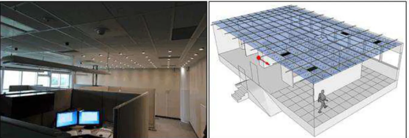
The test bed was housed in a larger experimental space 12.2 m x 7.3 m x 2.7 m, with an exterior wall facing west. During this study, the space was outfitted with six identical cubicle workstations (Figure 1). We used the north end of this experimental space as our LED test bed and installed LED lighting over one cubicle and the surrounding circulation space.
The LED lighting system was not intended to be a realistic lighting design for an office, but rather a platform to explore high-resolution control strategies in a proof-of-concept installation; successful concepts might then be developed into more realistic designs. For this purpose, we chose commercially-available LED spotlights. Each spotlight had four 1-watt LEDs with a typical power draw of 6.2 W on 24 V DC. The LED luminaires had a colour rendering index (Ra) of 85,
and a correlated colour temperature (CCT) of 3500 K; efficacy was calculated as 46 lm/W. Each LED was individually controllable via custom software using the DMX protocol, and could be dimmed to any level digitally and linearly. Each LED spotlight has a beam angle of 45.1º (Figure 2).
We distributed 72 LEDs on a 61 x 61 cm (2 x 2 ft.) grid following the ceiling tile layout. Each LED spotlight was co-located with a pair of inexpensive, commercial environmental sensors: a passive infrared (PIR) motion sensor with a relatively narrow field of view (38⁰ x 22⁰), and a photosensor (Figure 3). Data were gathered from these sensors at 20 Hz.
3.1.2 Occupancy Sensing System
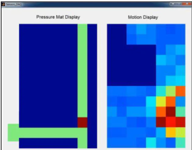
To locate a person or person(s) in the test bed requires processing data from multiple sensors in real time. When an occupant moves, all sensors with a field of view encompassing the occupant will send a signal to the lighting control system. Depending on the location of the occupant(s), the type of motion and the sensitivity of the sensors at that point in the field of view, these signals could be strong, weak or anything in between, and the strongest signal might not come from the sensor directly above the occupant. Figure 4 shows a screen capture from the test bed data acquisition software. The red square on the "Pressure Mat Display"3 (Figure 4-left)
shows the exact location of the occupant. Note how the occupancy signals from motion sensors are scattered on the "Motion Display" (Figure 4-right).
If a lighting control system were to control the lights directly by using raw data from the motion sensors, it would create an unacceptable luminous environment with rapidly changing light levels. We developed a proprietary algorithm to process the signals from all sensors to create a result that provided a more accurate estimate of the occupant’s location, and one that
transitions smoothly over time. This was supported by a set of experiments involving one or
3 When developing the control system, we used pressure mats on the floor to record the exact location of
occupants for comparison to the multiple motion sensor signals. The pressure mats were later disabled so the system relied entirely on motion sensor data.
6
several participants walking along a path with pressure mat sensors providing “ground truth” information. An example of such a trial is shown in Figure 5.
Figure 6 shows two time snapshots corresponding to a trial following the walking pattern of Figure 5. It is clear that raw motion sensor data (red) was noisy and also its relationship with the ground truth (blue) is not straightforward, creating false positive locations. On Figure 6-Left, two participants were at positions 5 and 7-8 along the path. Raw motion sensor data misplaced the participant at position 5, missed completely the participant at position 7-8 and produced a false positive location at position 10. The advanced algorithm we developed (aggregation function-green) correctly exhibited maximal responses at locations corresponding to the ground truth. On Figure 6-Right, participants were at positions 1-2 and 11 along the path. Raw motion sensor data (red) correctly identified the participants’ locations, but produced three false positives at positions 5, 7-8 and 13. The aggregation function (green) correctly exhibited maximal responses at locations closely corresponding to the ground truth with no false positives.
This work demonstrates the viability of very accurate occupancy sensing with a high-resolution sensor network. Energy savings may then accrue by providing electric lighting local to the occupants only.
3.1.3 Daylight Harvesting System
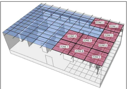
To simplify the control algorithms, we grouped the LED luminaires into nine zones as shown in Figure 7. Most zones contained nine luminaires, while the remainder contained six. Thus, when a dimming level was determined for a specific zone in any given scenario, all luminaires in each zone were dimmed to the same level but different from other zones. This sacrificed a small amount of potential savings from even higher-resolution control, but was a reasonable trade-off against system complexity.
To conduct automated daylight harvesting at the zone level we leveraged the readings of the photosensors co-located with each LED luminaire. At any system timestep we accessed the photosensor readings in the zone and subtracted the portion attributable to the electric lighting at its prevailing output value. This left the portion due to daylight, from which we calculated the contribution of daylight at the desktop level in that zone. By subtracting this value from the target desktop illuminance level we ascertained the amount of electric lighting required in the zone to maintain the target illuminance value, which may be higher or lower than the prevailing value. The new dimming level was enacted and the process was repeated every 5 seconds, and dimming between new control levels was enacted smoothly over the 5 seconds. We now describe how each of these steps was achieved.
To calculate the portion of the photosensor reading attributable to the electric lighting, we
performed an initial calibration without daylight in the space4. In this calibration all of the LEDs in
one zone were switched to full output and the response of each photosensor was recorded, this
7
was repeated zone by zone5. Because the LED output was linear and the photosensor
response to multiple sources was additive, this allowed us to calculate the electric light contribution at any of the 72 photosensors on the celling due to any combination of zone LED outputs:
{�� } = [ ]{ ��} = �� 7 , = �� 9 (Eq. 1)
Where, �� is a vector of 72 photosensor readings, [ ] is a 72 x 9 matrix, and its element is the reading of ith light sensor when the LEDs in zone j are on at full output, and �� is a value between 0 and 1 denoting the dimming level of the LEDs in zone j (0=off; 1=full power). Figure 8 shows the relationship between zones, sensors, control points, and calibration locations.
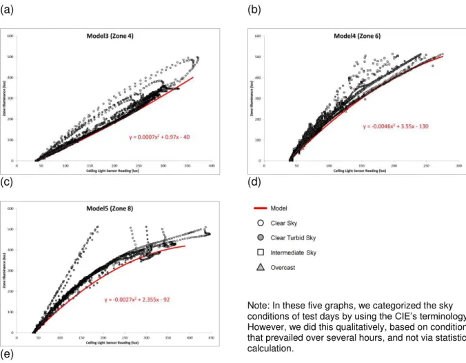
To calculate the illuminance contribution of daylight at the desktop level in that zone by the corresponding readings of the photosensors we used calibrations that were derived on multiple days with daylight in the space (under various sky conditions) and with the LEDs off. Li-Cor sensors were deployed to record desktop illuminance (E) in five zones, which were compared to the ceiling photosensor readings in the same zones every 1 minute. For stability, we used the average value of four or five photosensors above the control point of each zone to model the relationship, as shown in Table 3. The models were simplified as second-order polynomials:
� = ∙ �� + ∙ �� + (Eq. 2)
The calibration data and zone models are shown in Figure 9. Note that the polynomial was fit to the (approximate) lower bound of the data to ensure that in most cases the control algorithm was conservative, and provided a light level equal to or greater than the target illuminance. For zones without their own Li-Cor sensor and explicit model we assigned the model from a
neighbouring zone, also shown in Table 3; tests suggested this maintained adequate accuracy for this application, while reducing complexity.
Knowing the contribution of daylight to the desktop, the final step was to calculate the LED output required in each zone to ensure that the total desktop illuminance met the target. We calibrated the desktop illuminance in each zone against the LED light output from each zone. To do this, we placed a Li-Cor at desktop height at the control point in each zone in a non-daylit setting, and zone-by-zone and one-at-a-time, switched the LEDs to full power. This generated a matrix [ ] of illuminance contributions of the LEDs to each control point. This allowed us to calculate the illuminance vector at the 9 control points {� } due to a combination of zone LED outputs:
{� } = [ ]{ ��} , = �� 9 (Eq. 3)
Because our goal was to calculate the new control levels for the necessary combination of LED outputs to meet the target incremental illuminances from the LEDs {� }, we recast Eq. 3 as Eq. 4, to solve for the 9 dimming levels:
5 In a commercial application this process may be pre-programmed and run automatically during off
8
{ ��} = [ ]− {� } , = �� 9 (Eq. 4)
Where {� } is, known, the subtraction of the set-target illuminance and daylight illuminance by (Eq. 2) at zone j. Note that the raw solved control values might not be physically possible; i.e. <0 or >1, in which case values of <0 were set to zero, meaning that local illuminances might (slightly) exceed the total target; given the design of the space and lighting system, values of >1 were very rare.
In the final test scenarios of the high-resolution control system, occupancy sensing and daylight harvesting were combined. In this case, the occupancy algorithm indicated in which of the nine zones the occupant(s) were present, and electric lighting was provided to supplement the daylight available in the occupied zone(s) to reach to a target level, while keeping the other zone(s) at a pre-set value.
3.1.4 Automatic Control Trials
We completed a sequence of trials to illustrate the energy savings associated with advanced occupancy sensing only, high-resolution daylight harvesting only, and a combination of the two, compared to various baselines. For an open-plan space like the one used in our test bed, current North American codes do not require occupancy sensing during normal daytime working periods, and provide requirements only for whole-zone-level daylight harvesting.
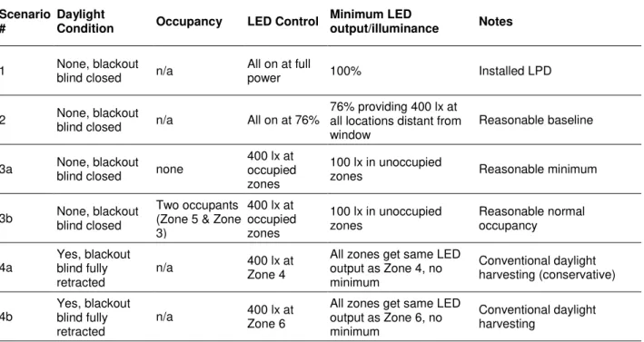
Table 4 describes each trial scenario. Scenario 1 represents the full installed LPD, in which the space is somewhat overlit. While Scenario 1 is not uncommon, a more reasonable baseline is Scenario 2, in which the LED luminaires were dimmed uniformly to provide 400 lx, a more typical office illuminance level, at all zones except Zones 1 & 2 (where light levels are lower in the no daylight condition due to lack of spill light from the adjacent zones). This dimming level, 76%, may be considered the reasonable maximum energy use for the space.
In Scenario 3, the advanced occupancy sensing approach was tested, in the absence of daylight. In Scenario 3a there were no occupants in the space, and the system adjusted to deliver 100 lx in all zones as a basic level of light for safe circulation. This may be considered the reasonable minimum energy use for the space. In Scenario 3b two occupants were
introduced to the space, one in the cubicle entirely covered by the lighting test bed, and another in the adjacent corridor, this representing a reasonable normal occupied condition for such a space. In this scenario, the system identified the occupied zones and dimed the luminaires such that there were 400 lx at desktop level in the occupied zones only, and 100 lx elsewhere.
Scenario 3b provided an estimate of the energy savings achieved from advanced occupancy sensing alone.
In Scenario 4, occupancy detection was switched off, and the focus was on the effect of daylight harvesting alone. Scenario 4a represented a conservative, conventional daylight harvesting system. In this scenario the goal was to ensure 400 lx on the desktop of the cubicle (Zone 4) from a combination of daylight and electric lighting. However, as with conventional whole-space systems, whatever dimming level was necessary for the Zone 4 control point was then adopted by all zones. This approach was very conservative because this desktop was in the rear half of the space, was enclosed by relatively high partitions, and relatively little daylight reached the desktop. Therefore, the target light level was maintained there, but the more open zones, or the
9
zones closer to the window, tended to be overlit. In Scenario 4b the single control point was moved to Zone 6, the same distance from the window as Zone 4, but without as much
shadowing from the surrounding partitions. The dimming level to maintain 400 lx in Zone 6 was lower, saving more energy, but that also had the potential to leave other zones underlit. This was even more the case in Scenario 4c, where the control point was moved to Zone 3, an open area closer to the window. Scenarios 4 served to illustrate the inevitable daylight harvesting trade-offs associated with a single sensor/control point in a diverse space.
Scenario 5 implemented the high-resolution daylight harvesting approach. Here the LED zones were dimmed (largely) independently, to different levels, to deliver 400 lx in all zones based on locally-measured daylight availability and geometry. A minimum dimming level of 5% was respected, to avoid excessive luminance contrast between luminaires in adjacent zones. This ensured adequate light levels maintained throughout the diverse space, while maximizing the energy savings.
Scenario 6 combined advanced occupancy sensing with high-resolution daylight harvesting, to illustrate the full potential of the new control features. In Scenario 6a there were no occupants in the space, and the system adjusted to deliver 100 lx in all zones; the difference compared to Scenario 3a was that if some of the 100 lx light level could be provided by daylight, the electric lighting was reduced accordingly and automatically (to a minimum of 5%). This scenario was another potential minimum baseline energy use for the space. Scenario 6b was the ultimate demonstration. Like Scenario 3b, the system delivered 400 lx to the occupied zones only, but if some of the 400 lx light level could be provided by daylight, the electric lighting was reduced accordingly and automatically (to a minimum of 5%). This scenario showed the full energy saving potential of the advanced system. These illustrative trials were conducted on a single day (November 24th) with an overcast sky condition.
3.2 Results
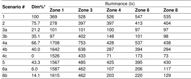
The key system performance metrics for the various scenarios are summarized in Table 5. Some particular comparisons from Table 5 are:
Scenario 6b vs. Scenario 2/Scenario 4a. This shows the full potential of the energy savings with the advanced control system. Relative energy use (expressed as mean dimming %) drops from 75.7% for Scenario 2, to 14.1%, or a saving of 81.4%, if one assumes a baseline with no controls. A baseline more similar to current energy code requirements for new buildings would be Scenario 4a, with a conservative, whole-space single sensor daylight harvesting system and no occupancy sensing. In this case, relative energy use drops from 66.7% to 14.1%, or a saving of 78.9%.
Scenario 4a vs. Scenario 5, a whole-space single sensor daylight harvesting system with a control point at Zone 4 provides a desktop illuminance close to the 400 lx target (428 lx) with a relative energy use of 66.7%, but other zones are overlit (e.g. Zone 6, at the same distance from the window, but in a more open geometry, at 537 lx, and Zone 3, closer to the window and open, at 753 lx). This illustrates the potential of the high-resolution control of Scenario 5, which meets the 400 lx target, without excessively exceeding it, in Zones 4 and 8 (425-430 lx), Zone 6 (395 lx), and Zone 3 (486 lx) with a
10
relative energy use of 43.3%. Scenario 4b, a whole-space single sensor daylight
harvesting system with a control point at Zone 6, matches Scenario 5 for energy savings (relative energy use of 40.0%), but still suffers from the single control point problem of satisfying illuminance requirements across the space. In this case the desktop
illuminance in Zone 6 is close to the 400 lx target (394 lx), but Zone 4 (287 lx) and Zone 6 (294 lx) are underlit.
Results varied on different days with different sky conditions, but the trends remained the same, with substantial energy savings using the advanced control features.
4. Discussion
4.1 Modelling of Shorter Occupancy Timeouts
Our calculation results were very similar to prior studies that estimated the potential benefits of a shorter timeout period (Table 6). This illustrates that the patterns of occupancy from our more recent datasets are not radically different from the patterns observed in prior decades, and that the energy savings potential is supported by replication.
A frequent concern with garnering more energy savings with controls using fluorescent systems is the reduction in lamp life that may occur with more frequent switching [Bullough, 2000]. The number of on-off cycles and associated runtimes for our modelled data in the various scenarios are shown in Dikel & Newsham [2014]. Because the present article is specific to LED systems, it is suffice to say that, in contrast to fluorescent light sources, switching frequency is not a
determining factor in LED life [US DoE, 2009].
Although focussed on energy use, we also calculated the average power consumption vs. time of day associated with shorter timeouts. This illustrates the actual power draw per area, which may be termed the equivalent or controlled LPD [Galasiu et al., 2007; Wen et al., 2015]. Figure 10 shows the effect on the equivalent LPD of two timeout periods of interest, derived from the two data samples: 20-minute timeout on 5-min data (Scenario 3b), 20-minute timeout on 15-sec data, and 1-minute timeout on 15-sec data (Scenario 5); data are averaged over the 60 sample days (6 WS x 10 days each) applicable to each dataset. It is apparent from Figure 10 that the substantial energy savings in Table 2 come in large part from the partial occupancy periods in the first half of the morning and the last half of the afternoon; the reductions in LPD in the middle of the day are more modest. Indeed, for a 20-minute timeout on 15-sec data the peak (13.2 W/m2) barely drops below the baseline of all lighting on during the occupied period (13.5 W/m2).
However, for a 1-minute timeout on 15-sec data the peak drops to 12.4 W/m2, or a reduction of
8%. Thus the LPD reduction is much lower than the overall energy saving, but is nevertheless meaningful. Greater reductions would be expected when averaging over a larger sample of offices with a greater diversity of occupancy.
Prevailing North American codes require occupancy sensing (or similar) for private offices, while some offer an optional incentive for using the technology in the open-plan [e.g. CEC, 2012: Table 140.6-A]. Our modelling was done in the context of an open-plan office, because the dedicated luminaire and multi-sensor approach makes reliable, workstation-specific occupancy
11
sensing viable in such shared spaces. This unlocks the potential to realize substantial savings in the most common office space type.
4.2 Automatic Control Trials in the Test bed
Overall, the novel control system worked very well, and supports a substantial reduction in lighting energy use compared to conventional control systems, and particularly those embodied in current North American energy codes for open-plan office spaces.
One limitation with the system, as proposed, was the need for calibration using desktop illuminance sensors to derive the matrices in Eq. 2 and Eq. 3. This challenge is not unique to our proof-of-concept system, but is common to existing conventional daylight harvesting systems too. The sensors for Eq. 3 only need to be in place for a short period to cycle through zone dimming levels, but for Eq. 2 the sensors would have to be in position for several days to capture different sky conditions and sun angles. As sensors become cheaper and more numerous, it is not unreasonable to expect that deploying a temporary network of sensors for this purpose might be less of a barrier in the future. Another option in the short-term may be to take the most conservative curve from Figure 9, which was measured for a variety of sky conditions and local geometries, and pre-load that into all zones deployed in a system elsewhere, and allow for local adjustment of equation coefficients. Again, such a process is already practiced with conventional daylight harvesting installations, where base dimming levels are set at night, and dimming sensitivity to the presence of daylight and respecting local
conditions is done through the adjustment of “gain” controls, or similar. 4.3 Additional Applications for a High-resolution Sensor Network
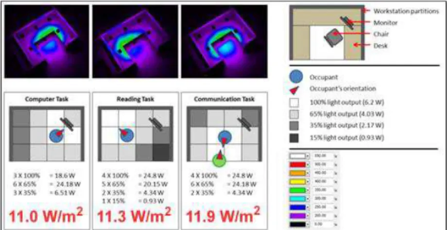
Additional advanced lighting control features may be supported by this approach, with the potential for further energy savings. With multiple light sources and sensors per workstation, it might be possible to automatically tune lighting spatially within a workstation to certain tasks [Fischer et al., 2012]. This general concept was explored by Chen et al. [2013] and reached up to 80% energy savings compared to their benchmark condition with no lighting control.
Examples are shown in Figure 11, illustrating lower LPDs than the non-task tuned value (13.5 W/ft2).
In addition to lighting control, other building environmental systems may leverage the data from the lighting system sensors to optimize their own service delivery. For example, better dynamic matching of HVAC service to space occupancy has been estimated to save 10-60% of HVAC energy [Li et al., 2012]. Beyond energy savings, there are other potential value-added
applications for high-resolution occupancy data. One possibility is space utilization: if part of an office floorplate is used infrequently that might indicate an opportunity for savings via space consolidation. An organization might also observe motion sensor data to confirm whether expected patterns of communication were taking place between business units. Another application is safety and security: if no legitimate occupancy is expected in a space at a particular time an intruder can be detected immediately. Another example might be to guide emergency services personnel to occupied spaces during an urgent event.
12
Although this technology may have the potential for substantial energy savings and other benefits, the effect of such a control system on the occupants well-being should be evaluated in human factors studies before applying this approach to real commercial office spaces.
5. Conclusion
In this study, we have demonstrated substantial energy savings potential (and other potential benefits) associated with a high-resolution sensor network combined with a spatially-defined and granular LED lighting system. Although some of these energy benefits have been
articulated before, we argue that they were not practical, particularly in open-plan offices, with conventional fluorescent technology and historically-available sensors. First, the form factor of LED packages enables a higher granularity of light sources in a space with inherent dimmability. Second, the networked and solid-state nature of LEDs encourages the co-location of sensors to provide a real-time, high-resolution sensor network; such sensor technology has also declined rapidly in price in recent years. A high density of sensors supports more accurate occupancy sensing, permitting substantially shorter timeout periods, and localized daylight harvesting, to ensure that electric lighting is only provided where it is needed, when it is needed, and in the amount it is needed, within zones of a few square metres. Such sensor data could also be leveraged for more efficient HVAC control, space utilization, and safety and security functions. These additional features might help offset the incremental cost of such a lighting system.
6. Acknowledgements
This study is a product of the NRC projects A1-002833, Solid-state Lighting: Enhancing Energy Efficiency and Ensuring Market Acceptance, and A1-006219, Solid-State Lighting: Enhancing Energy Efficiency by Facilitating Equivalent Lighting Power Densities, which are part of the NRC High Performance Buildings program. Financial support for the former was provided by the EcoEnergy Innovation Initiative (managed by Natural Resources Canada), Natural Resources Canada - Office of Energy Efficiency, the Conservation Fund of the Ontario Power Authority (now merged with the Ontario Independent Electricity System Operator), and the National Research Council Canada. Financial support for the latter was provided by BC Hydro and the National Research Council Canada. The authors thank colleagues Jennifer Veitch for her overall project management of A1-002833, guidance and advice, Anca Galasiu for her
assistance with occupancy data and lighting simulations, and Trevor Nightingale for his support. We are also grateful for the support of Cristian Suvagau and Toby Lau of BC Hydro.
7. References
ASHRAE, ANSI/ASHRAE/IES Standard 90.1-2010 (I-P Edition), Energy Standard for Buildings Except Low-Rise Residential Buildings, ASHRAE: Atlanta, GA.
13
Baylon, D.; Storm, P. 2008. Comparison of commercial LEED buildings and non-LEED buildings within the 2002-2004 Pacific Northwest commercial building stock. Proceedings of ACEEE Summer Study on Energy Efficiency in Buildings (Pacific Grove, CA), 4.1-4.12
Bullough, J.D. La vita è bella (lamp life). Lighting Futures, 2000. 4.
Caicedo, D.; Pandharipande, A.; Leus, G. 2011. Occupancy-based illumination control of LED lighting systems. Lighting Research & Technology, 43, 217-234.
California Energy Commission (CEC). 2012. 2013 Building Energy Efficiency Standards for Residential and Nonresidential Buildings, Part 6. Available from: http://www.energy.ca.gov/2012publications/CEC-400-2012-004/CEC-400-2012-004-CMF-REV2.pdf
Canadian Commission on Building and Fire Codes (CCBFC). 2011. National Energy Code of Canada for Buildings (1st ed.). National Research Council of Canada: Ottawa, ON.
Chen, N.H.; Nawyn, J.; Thompson, M.; Gibbs, J.; Larson, K. 2013. Context-aware tunable office lighting application and user response. Proceedings of SPIE - The International Society for Optical Engineering, LED-based Illumination Systems, 8835.
Dikel, E.E.; Newsham, G.R. 2014. A quick timeout: unlocking the potential energy savings from shorter time delay occupancy sensors. LD+A (December), 54-56.
Fischer, M.; Wu, K.; Agathoklis, P. 2012. Intelligent illumination model-based lighting control. 32nd International conference on Distributed Computing Systems Workshop. (Macau, China).
Galasiu, A.D., Newsham, G.R., Suvagau, C., Sander, D.M. 2007. Energy saving lighting control systems for open-plan offices: a field study. Leukos, 4 (1), 7-29.
Galasiu, A.D.; Newsham, G.R. 2009. Energy savings due to occupancy sensors and personal controls: a pilot field study. Lux Europa , 11th European Lighting Conference (Istanbul, Turkey).
Illuminating Engineering Society of North America. 2013. ANSI/IES RP-1-12: Recommended Practice for Office Lighting, Illuminating Engineering Society.
Li, N.; Calis, G.; Becerik-Gerber, B. 2012. Measuring and monitoring occupancy with an RFID based system for demand-driven HVAC operations. Automation in Construction, 24, 89-99.
Maniccia, D.; Tweed, A.; Bierman, A.; Von Neida, B. 2001. The effects of changing occupancy sensor timeout setting on energy savings, lamp cycling and maintenance costs. Journal of Illuminating Engineering Society, 30(2), 97-110.
Newsham, G.R.; Xue, H.; Valdes, J.J.; Scarlett, E.; Arsenault, C.; Burns, G.J.; Kruithof , S.; Shen, W. 2015. Factors affecting the performance of ceiling‐based PIR occupancy sensors in offices. IESNA Annual Conf. (Indianapolis, USA), pp. 1-5.
Pandharipande, A.; Caicedo, D. 2011. Daylight integrated illumination control of LED systems based on enhanced presence sensing. Energy and Buildings, 43, 944-950.
Richman, E.E.; Dittmer, A.L.; Keller, J.M. 1996. Field analysis of occupancy sensor operation: parameters affecting lighting energy savings. Journal of the Illuminating Engineering Society, 25(1), 83-92.
Roisin, B.; Bodart, M.; Deneyer, A.; Herdt, P.D. 2008. Lighting energy savings in offices using different control systems and their real consumption. Energy and Buildings, 40(4), 514-523.
Tiller, D.K.; Guo, X.; Henze, G.P.; Waters, C.E. 2009. The application of sensor networks to lighting control. Leukos, 5(4), 313-325.
14
Tiller, D.K.; Guo, X.; Henze, G.P.; Waters, C.E. 2010. Validating the application of occupancy sensor networks for lighting control. Lighting Research & Technology, 42(4), 399-414.
U.S. Department of Energy (USDoE). 2009. Lifetime of White LEDs. Available from: http://apps1.eere.energy.gov/buildings/publications/pdfs/ssl/lifetime_white_leds.pdf
van de Meugheuvel, N.; Pandharipande, A.; Caicedo, D.; van den Hof, P.P.J. 2014. Distributed lighting control with daylight and occupancy adaptation. Energy and Buildings, 75, 321-329.
Von Neida, B.; Maniccia, D.; Tweed, A. 2001. An analysis of the energy and cost savings potential of occupancy sensors for commercial lighting systems. Journal of Illuminating Engineering Society, 30(2), 111-122.
Wen, Y.-J.; Seeger, K.; Maniccia, D. 2015. Toward a performance-based energy code. LD+A (July), 44-47.
Williams, A.;Atkinson, B.; Garbesi, K.; Page, E.; Rubinstein, F. 2012. Lighting Controls in Commercial Buildings. Leukos, 8(3), 161-180.
15
Figure 1. Left: Photo of the test bed. Right: Axonometric view.
Figure 2. Polar candela plot of the LED spotlights.
16
Figure 4. Screen capture from the data acquisition software. Note: Each colour on the “Motion Display” (right) represents a level of signal strength, from dark blue (weakest) to dark red (strongest).
Figure 5. Left: Example of a walking pattern defined by two participants starting at pressure mat positions 2 and 19 and walking towards each other. Red arrows indicate walking directions along the path. Right: A
person is walking from mat position 2.
Figure 6. Snapshots of two 1D data distributions at two different times for the walking trial. Note: X-axis represents the zones of pressure mats. Y axis represents the amplitude of the occupancy signals. Red: Raw
motion sensor data, Blue: Pressure mat sensor values (ground truth) and Green: Aggregation function applied to the raw motion sensor data.
17
Figure 7. The nine control zones used in the final automated test bed.
Figure 8. The relationship between zones, sensors, control points, and calibration locations. The large squares, Z1 to Z9, indicate the 9 zones. The small squares numbered 1-72 are the locations of the LED luminaires and sensors. The Control Point (CP), shown by blue squares, is the location in each zone where we calculated the illuminance of the zone; generally at the center of the zone. For initial modelling and calibration purposes, 5 Li-Cor illuminance sensors were installed in 5 key zones, shown by blue circles.
18 (a) (c) (b) (d) (e)
Note: In these five graphs, we categorized the sky conditions of test days by using the CIE’s terminology. However, we did this qualitatively, based on conditions that prevailed over several hours, and not via statistical calculation.
19
Figure 10. Average power draw (equivalent LPD) by time of day, under various control options. The red line is the installed power assuming no controls, and a 7:00 A.M.-7:00 P.M workday. The black line shows the calculated LPD with individual workstation occupancy sensing with a 20-minute timeout using 5-minute data
(Scenario 3b); the blue line is the calculated LPD with individual workstation occupancy sensing with a 20-minute timeout, using 15-second data; the green line is the calculated LPD with individual workstation
occupancy sensing with a 1-minute timeout, using 15-second data (Scenario 5).
20
Table 1. Modelled occupancy-based control scenarios.
Scenario 1, Timer control: Typical of current lighting practice in older commercial buildings where
lighting is centrally controlled: all lights are switched on in the morning before the first occupant is expected to arrive, and are switched off in the evening after the last occupant is expected to leave; lights are on for 12 hours, between 7:00 A.M. and 7:00 P.M.
Scenario 2, Space-level occupancy sensor: All lights are on from the arrival of the first occupant to the
departure of the last occupant (with a 10-minute timeout after the last occupant leaves). This represents a system with a single occupancy sensor for multiple occupants, or an adaptive centrally-controlled system, or disciplined manual control.
Scenario 3, Single occupancy sensor for each workstation (with various timeout periods):
Scenario 3a, 30-minute timeout: This scenario represents the upper limit of the requirement for private
offices (but not open plan) in current energy codes. Scenario 3b, 20-minute timeout: likely to be the upper timeout limit in the next generation of energy codes. Scenario 3c, 10-minute timeout: A more aggressive setting for existing sensor technology. In all cases, lighting is switched back on when occupancy is detected.
Scenario 4, High-resolution sensors, without timeout: 12 occupancy sensors per workstation were
leveraged for perfect sensing. Scenario 4a: The first occupancy data set, with 5-minute frequency, was used. Scenario 4b: The second occupancy data set, with 15-second frequency, was down-sampled (averaged) to 5-minute frequency. This sub-scenario allows us to test the similarity of the two occupancy data sets. Scenario 4c: The second data set was used at the original 15-second frequency, facilitating energy savings for absences less than 5 minutes. Lighting is switched back on when occupancy is detected.
Scenario 5, High-resolution sensors with 1-minute timeout period: Similar to Scenario 4c, except
that a 1-minute timeout was introduced, adding a safety factor against residual false negatives.
Table 2. Energy consumption calculation results of five scenarios during 250 workdays.
Total energy consumption for 250 days in kWh
Data from
: The cubicle area
(based on 5-min. data recorded frequency)
Individual workstations
(based on 15-sec. data recorded frequency) S c en ar ios : 1 2 3a 3b 3c 4a 4b 4c 5 Li g hts on for 1 2 h o urs Li g hts on fr om t he f ir s t to the l as t o c c up an t Ind iv idu al oc c up a nc y s en s or i n ea c h w ork s tat io n Ind iv idu al oc c up a nc y s en s or i n ea c h w ork s tat io n Ind iv idu al oc c up a nc y s en s or i n ea c h w ork s tat io n Hi gh r es ol uti on s en s ors wi th ou t t im eo u t Hi gh r es ol uti on s en s ors wi th ou t t im eo u t (5 -mi nu te inte rv a l) Hi gh r es ol uti on s en s ors wi th ou t t im e t ime ou t (15 -s ec on d i nte rv a l) Hi gh r es ol uti on s en s ors wi th 1 -mi nu te t ime ou t T ime out P eri od : None None 30 m inu tes 20 m inu tes 10 m inu tes
None None None 1 m
inu
te
Mean Energy
21 Savings
vs.
Scenario 1 - 15.0% 22.2% 25.5% 31.6% 39.4% 42.2% 48.6% 45.8%
Scenario 3b - - - - 8.2% 18.7% 22.4% 30.2% 26.0%
Scenario 1 forms the fundamental baseline for these calculations as the assumption of no controls has been the base case for most of the historical studies to which we can compare our results. However, given the contemporary energy code regime, Scenario 3b might be a more appropriate baseline to support further code development. Note, Scenarios 4a and 4b are the only two conditions in which the two occupancy datasets were used for the same calculation timeframe (5 minute frequency). The results of these scenarios differed by less than 5%, which gave us confidence that the two data sets were similar enough that the second data set may be used to extend the results to shorter timeframes.
Table 3. Zones, Photo sensors and Daylight Models.
Zone # Model Photosensors for model
1 Model1 65 66 67 69 2 2 62 63 64 72 3 Model2 5 55 57 58 59 4 Model3 35 46 47 49 5 37 43 44 45 51 6 Model4 8 40 41 42 54 7 Model5 19 20 21 33 8 16 22 23 24 30 9 11 13 25 26 27
Table 4. Advanced lighting control scenario descriptions. Scenario
#
Daylight
Condition Occupancy LED Control
Minimum LED
output/illuminance Notes
1 None, blackout
blind closed n/a
All on at full
power 100% Installed LPD
2 None, blackout
blind closed n/a All on at 76%
76% providing 400 lx at all locations distant from window
Reasonable baseline
3a None, blackout blind closed none
400 lx at occupied zones
100 lx in unoccupied
zones Reasonable minimum
3b None, blackout blind closed
Two occupants (Zone 5 & Zone 3) 400 lx at occupied zones 100 lx in unoccupied zones Reasonable normal occupancy 4a Yes, blackout blind fully retracted n/a 400 lx at Zone 4
All zones get same LED output as Zone 4, no minimum Conventional daylight harvesting (conservative) 4b Yes, blackout blind fully retracted n/a 400 lx at Zone 6
All zones get same LED output as Zone 6, no minimum
Conventional daylight harvesting
22 4c Yes, blackout blind fully retracted n/a 400 lx at Zone 3
All zones get same LED output as Zone 3, no minimum Conventional daylight harvesting 5 Yes, blackout blind fully retracted n/a 400 lx at each zone 5% High-resolution daylight harvesting 6a Yes, blackout blind fully retracted none 400 lx at occupied zones 100 lx in unoccupied
zones, minimum 5% Reasonable minimum
6b
Yes, blackout blind fully retracted
Two occupants (Zone 5 & Zone 3) 400 lx at occupied zones 100 lx in unoccupied zones, minimum 5% Reasonable normal occupancy, full potential of advanced system
Table 5. Advanced lighting control scenarios, system performance metrics.
Scenario # Dim%* Illuminance (lx)
Zone 1 Zone 3 Zone 4 Zone 6 Zone 8
1 100 369 528 526 547 535 2 75.7 278 397 397 413 404 3a 21.2 101 101 100 97 97 3b 35.1 97 402 148 101 98 4a 66.7 1708 753 428 537 438 4b 40.0 1642 638 287 394 294 4c 0 1526 433 71 173 73 5 43.3 1567 485 425 395 430 6a 6.0 1587 462 107 206 117 6b 14.1 1615 462 203 220 129
* Depending on the control scenario, this could be the same dimmer setting for all zones or a mean value of differing dimmer settings across the whole space (where 100 represents lights fully on, and 0 represents all lights off).
Table 6. Energy saving percentages of different timeout periods found in this study and other studies, compared to having no occupancy sensing.
Source Number and Type of the Sample Spaces
Time Period to Record Data
Time Delay (minutes)
30 20 15 10 5 2 1
Von Neida
et al. [2001] 37 Private Offices
6:00 a.m.-
6:00 p.m. N/A 22 24 28 32 N/A N/A Richman et
al. [1996] Average of 4 offices N/A 23.3 30.3 41.3 58.5 76 N/A Maniccia et
al. [2001] N/A 28 31 34 38 N/A N/A
This study –
Simulation
Six workstations 7:00 a.m. -