Antenna beamforming for infrastructureless wireless networks

Antenna Beamforming for Infrastructureless

Wireless Networks

by

Elizabeth C. Godoy

Submitted to the Department of Electrical Engineering and Computer Science in Partial Fulfillment of the Requirements for the Degree of

Master of Engineering in Electrical Engineering and Computer Science at the

MASSACHUSETTS INSTITUTE OF TECHNOLOGY May 2007

© 2007 Massachusetts Institute of Technology. All rights reserved.

Author

Department of Electrical Engineering and Computer Science May 31, 2007

\

I

'a

Certified b

Vincent W. S. Chan

Joan and Irwin M. Jacob Professor of EECS and Aero/Astro Director, L for Information and Decision Systems

/ · Thesis Supervisor

-~- -.

Y---Accepted by

Arthur C. Smith Professor of Electrical Engineering Chairman, Department Committee on Graduate Theses

ARCHIVES

OCT 0 3 2007LIBRARIES

LIBRARIES

Antenna Beamforming for Infrastructureless

Wireless Networks

by

Elizabeth C. Godoy

Submitted to the Department of Electrical Engineering and Computer Science on May 31, 2007, in partial fulfillment of

the requirements for the degree of

Master of Engineering in Electrical Engineering and Computer Science

Abstract

Our work studies the impact of antenna beamforming on the performance of infrastructureless wireless networks. Based on examination of the beampattern for a uniform circular antenna array (UCAA) utilizing beamforming under a constraint on maximum average transmit power, we approximate achievable user data rates as a function of the number of antenna elements, and we examine the behavior of these rates in a simple network with varying noise power and interference and with different scheduling of user transmissions. We find that user data rates increase with the number of antenna elements up to a point of saturation determined by the antenna size and carrier wavelength. Moreover, in some cases that we outline, judicious scheduling of user transmissions can increase achievable data rates.

Thesis Supervisor: Vincent W. S. Chan

Title: Joan and Jacob Professor of EECS and Aero/Astro Director, Laboratory for Information and Decision Systems

Acknowledgements

I would like to thank Lillian Dai and Professor Chan for their unwavering support and guidance, without which this work would not have been possible. Lillian's help at every step in the process of creating this thesis proved invaluable. In addition, I am fortunate to have had Professor Chan as an advisor and am grateful to him for providing me with the opportunity to do this work and also for offering his insights and wisdom. I am also grateful to DARPA for providing the financial support for this research. Thank you, as well, to my officemates and the administrative staff, who have made my time at LIDS enjoyable.

Most importantly, thank you to my parents for providing me with the foundation to learn and grow. To my parents, brother and family: you are the source of my strength.

Finally, thank you to my friends for making my world at MIT entertaining and memorable. Your support and friendship have kept me sane and smiling.

Table of Contents

4 Antenna Radiation Field Review 22

4.1 Aperture Radiation Field --- --- 22

4.2 Radiated Power and Directive Gain 26

5 Aperture and Array Beamforming 28

5.1 Continuous Aperture Beamforming --- 28 5.2 Multiple Element Array Beamforming --- 31

5.2.1 UCAA Directivity --- 35

5.2.2 Aperture & Array Beamforming Revisited ... 41

5.3 Receive Beamforming --- 42 5.4 Beamforming and Power Allocation for Multiple User Transmissions . 44

6 Beam Characteristics, Sidelobe Behavior, and Interference in the

Wireless Network 48

6.1 Beampattem and Beamwidth --- 48 6.2 Spatial Aliasing in the UCAA Beampattern ... 52 6.3 Sidelobe Levels of a UCAA Beampatternm . ... 55

6.3.1 Maximum Sidelobe Level 56

6.3.2 Average Sidelobe Level - ---. 59

6.3.3 Minimum Sidelobe Level 63

6.4 Beam Parameter Summary --- 64

7 Acheivable Data Rates for a Three-User Network 67

7.1 U ser D ata Rate . ... ... .. . . ... .. ... 67

7.2 Data Rates with User Scheduling ... 76 7.3 Comparison of Average Data Rates for Scheduling Schemes A, B, & C ... 82

8 Conclusions & Future Work 89

List of Figures

2-1 A satellite rectangular aperture antenna serving users on the Earth. - - - 14 2-2 An infrastructureless wireless network of users with antenna arrays on the ground. 14 3-1 Uniform Circular Antenna Array (UCAA)... 18 3-2 Uniform circular antenna array (UCAA) and continuous ring aperture,. ... 21 4-1 Diagram of a single antenna element located at r' and a point of observation in

the farfield at r0 . . . . 2 4

4-2 Coordinate System. ... 26

5-1 UCAA Directivity versus the number of antenna elements for different antenna

sizes. 36

5-2 Maximum Array Directivity as a function of the ratio of antenna size to carrier

wavelength, 2R/2. -- - -- - -- - -- - -- - -- - -- - -... -37 5-3 Calculated UCAA directivity (5.17, solid), with linear approximation (5.19, dashed).

39 5-4 Maximum UCAA directivity, calculated (blue) and approximated (red) as a function

of the ratio of antenna size to carrier wavelength, 2R/ .-... ... .40

6-1 Beampattern for a UCAA of radius R = { with Ns,, elements ...-... 49 6-2 Sample UCAA beampattern with 3dB, 10dB, 15dB and 2/2R beamwidths. ---50 6-3 UCAA beamwidth as a function of the ratio of antenna diameters to carrier

wavelength, 2R/A. ...- - 51

6-4 Comparison of UCAA beamwidths for two different ratios of antenna diameter to carrier wavelength (normalized polar beam plots). ---_--- 52

6-5 Polar beam plots: Nsa, = 13,2R/A = 2,

b

6-6 UCAA beampattemrn as a function of N, Nsat = 40,2R/A = 6, 0₀ = . ... 55

2

--

---6-7 Ratio of Maximum Sidelobe-to-Peak UCAA beam level as a function of array

sparsity N/Nsa , shown with the approximation 'max = 1.16 - N/ Ns (black). ... 58

6-8 Plots of the ratio of Maximum Sidelobe-to-Peak UCAA beam level as a function of array sparsity N/ for different ratios of antenna size to carrier wavelength.

/•sat

Plots shown with the approximation ( = 1.₁₆ -N/N (green) ... 59

/ _Nsat

6-9 Ratio of Average Sidelobe-to-Peak UCAA beam level as a function of array sparsity

/N, (linear scale), shown with the approximation a =N (dashed) ... 60

6-10 Ratio of Average Sidelobe-to-Peak UCAA beam level as a function of array

sparsity N Nsat (dB scale), shown with the approximation ave = 1N (dashed). 61

6-11 _{Plots of the ratio of Average Sidelobe-to-Peak UCAA beam level as a function of}

array sparsity N/ for different ratios of antenna size to carrier wavelength. /Nsat

Plots shown with the approximation ra, = 1_{N (dashed green), ... 62}

6-12 Plots of the ratio of Average Sidelobe-to-Peak UCAA beam level (dB scale) as a function of array sparsity N/N for different ratios of antenna size to carrier

Nsat

wavelength. Plots shown with the approximation ave = YN (dashed green)... 63

7-1 Three Node Network. 68

7-2 User data rates under Scheme A without scheduling for minimum, average and

maximum interference as a function of noise power density, =1 [W/m2 ...73

7-3 Rate versus the number of antenna elements with varying bandwidth for Imi, (solid),

a,,ve (dashed) & Ima (dotted), 1 [W ] (Na,= 19)... .. 75

7-4 Data rates as a function of the number of antenna elements for zero interference and

7-5 Data rate as a function of the number of antenna elements for the severely

interference-dominated case, No = 10-[O'4P t i[W/m ], (N sat 19). ... .84

7-6 Data rates (A, solid; B, dashed; C dotted) as a function of the number of antenna elements for minimum, average and maximum interference with

increasing bandwidth, -= [•/ m 2] (Nsat= 19). 85

7-7 Data rates as a function of the number of antenna elements for average interference and varying noise power density, ot= 1

[/m

]

7-8 Data rates as a function of the number of antenna elements for average interference and varying noise power density, ot = 1 [W _] (Nsat=19) . --- 87

List of Tables

6.1 UCAA beamparameter summary ... 64

6.2 Interference gains. ... 65

7.1 Interference-dominated and large bandwidth rates as a function of N. ... 74

7.2 Summary of average user data rate for scheduling schemes A, B, and C. ... 81 7.3 Summary of comparison between data rates under Schemes A, B, and C. ._ . 88

Chapter 1

Introduction

Technological advances in wireless communications over the past few decades have revolutionized the way by which people interact. From cell phones to any of the assortment of devices used for wireless Internet access, it has never been easier to remain connected to the global telecommunication network. One technological advance that has received much attention in the wireless communications field is multiple antenna element systems. Such systems find applications for both optical and radio frequency (RF) antennas in satellite, cellular, and ad-hoc wireless communications. In contrast to wireless devices that use a single omnidirectional or directional antenna, wireless devices that use multiple transmit and/or receive antenna elements can better combat channel fading through diversity, and attain higher data throughput by concentrating power in desired directions and suppressing interference in undesired directions.

One particular way of utilizing multiple antenna elements in wireless networks is antenna beamforming. By controlling the phase and amplitude of the signal field at each antenna element, the radiated electromagnetic (EM) field can be patterned to have high antenna gains in desired directions and low antenna gains in undesired directions. Such a multiple antenna element system is termed a beamforming antenna array.

Antenna beamforming has found a diverse range of applications, including satellite [1] and cellular [2]-[4] wireless communications. In recent years, many proposed using antenna arrays in ad-hoc wireless networks [5]-[16]. Since many ad-hoc wireless networks are interference-limited [17], antenna arrays can significantly increase network

data rates over systems with omnidirectional antennas. However, practical implementations of antenna arrays for such networks are few and far in between. For cellular networks, directional and sectoral antennas are typically used. For mobile wireless networks, one of the main challenges is the lack of location tracking in conventional ad-hoc wireless networks, making it difficult to adapt the antenna radiation pattern to the changing user locations. Proactive Mobile Wireless Networks, as presented in [18], offers an example of a type of infrastructureless wireless network in which the positions of wireless users are available from localization and trajectory prediction. With these additional capabilities, antenna arrays can be more effectively used in a mobile wireless network environment.

The primary goal of this thesis is to study the impact of antenna beamforming on the performance of infrastructureless wireless networks. We present analytical expressions for the radiated field of an antenna array as a function of the array size and number of antenna elements. With these expressions, the antenna directivity; interference, and achievable data rates in a multi-user environment can be found. In addition to beamforming, we also examine the effects and address the potential benefits of scheduling transmissions in the network to further reduce interference. Since the joint antenna beamforming, power allocation, and scheduling problem does not lend itself to analytical studies, instead of resorting to numerical and algorithmic studies, we attempt to gain some insights on the achievable data rates by studying a simple network with three users located at the vertices of an equilateral triangle.

Our contributions include:

* A model approximating directivity and interference levels generated by a single antenna array.

* A study of the impact of interference on achievable data rates in a simple three-user network.

* Insights into how beamforming, power allocation, and scheduling affect user data rates in infrastructureless wireless networks.

This dissertation is organized as follows. We present the problem setup in chapter 3 and outline the models and assumptions that we use throughout our work. Chapter 4 reviews the physics of radiating antennas while Chapter 5 examines beamforming for aperture and array antennas in an infrastructureless wireless network context. Chapter 6 makes approximations to the beam sidelobe levels based on the density of array elements and then uses these approximations to analyze interference in the network. Chapter 7 summarizes the beamforming, power and interference analyses in the previous chapters and examines the achievable data rates in a simple network. The last section of Chapter 7 examines achievable data rates and compares the network performance for different power allocation and scheduling schemes. Finally, Chapter 8 concludes our work and proposes future research directions based on our findings.

Chapter 2

Background

This thesis is primarily motivated by [1] on joint antenna array beamforming and scheduling for satellite communications. The work in [1] examines beamforming for satellite transmissions from an antenna aperture to multiple users on Earth. An antenna aperture, in the context of [1] and as used in this thesis, is an antenna of finite size with an infinite number of infinitesimal antenna elements. In addition to beamforming, [1] also considers the benefits of scheduling in scenarios where users experience a high level of interference. In this thesis, we seek to extend the analysis presented in [1] to an infrastructureless wireless network scenario within the architectural framework of Proactive Mobile Wireless Networks.

The antenna model used in [1] cannot be directly carried over to our problem for two reasons. First, for satellite communications, the antenna on the satellite in space is transmitting to users on the Earth, approximately normal to the antenna, as shown in Fig. 2.1. In [1], the antenna aperture radiation field is taken directly from the results of scalar diffraction theory with the Fraunhofer approximation. In scalar diffraction theory, the field at the aperture is adequately modeled by "secondary radiating sources," each radiating EM fields that are maximized in the direction normal to the aperture and diminished in the directions away from the normal [19]. For the scenario in [1], the directivity of these secondary radiating sources in the direction of the users is approximately constant since the users are all located around a region close to the normal direction. For infrastructureless wireless network communications, users transmit to and

receive from other users on the same plane, as shown in Fig. 2.2. For simplicity, in this thesis, we examine beamforming for circular arrays oriented parallel to the ground so there is rotational symmetry in the radiated beam pattern in any direction.

iSatellite Antenna

n, normal

Fig. 2.1. A satellite rectangular aperture antenna serving users on the Earth.

(x,y and z are the axes labels in the Cartesian coordinate system, ni is the normal vector to the antenna)

* 0**. o O>.o °°° goes" ggo.o OO0 O 0 OO0 O 0 ·4 O 0 01 User Antenna :.'* see Earth

Fig 2.2. An infrastructureless wireless network of users with antenna arrays on the ground.

Second, [1] considers beamforming for a continuous antenna aperture in which the phase and amplitude of the antenna field can be adjusted at all points on a continuous surface. Our work, on the other hand, addresses beamforming for a discrete array of antenna elements, with a continuous aperture as a limiting case. As we will discuss in Chapter 3, our study will focus only on the radiation pattern due to array geometry. In doing so, each point on the array is appropriately modeled as an isotropic radiating source as opposed to a secondary source with directivity. In extending the beamforming analysis in [1] to infrastructureless networks, the directive gains of a discrete array antenna approach that of a continuous aperture of the same size.

Like [1], we consider an idealized channel model without fading or scattering in the environment in order to understand the basic properties and effects of beamforming on achievable user data rates. We also consider beamforming with scheduling among the users to explore the potential benefits of scheduling user transmissions in scenarios with different noise and interference levels.

Chapter 3

Problem Set-Up

This thesis seeks to study the impact of antenna arrays on infrastructureless wireless network performance, albeit in an idealized setting. The network model under consideration will be described in this chapter. This includes a discussion of the wireless scenario and several simplifying assumptions. We will also describe the antenna model including the particular antenna geometry and beamforming scheme that we consider.

3.1 Network Model

We consider a network of M users, indexed by j = 1,...M, each operating in a

planar surface as shown in Fig. 2.2. These users may be mobile and are assumed to have means to determine their relative locations at any time. The users (or nodes) are wirelessly enabled and automatically discover other nodes within their communication range. In addition, each user is equipped with a multiple antenna element array and utilizes beamforming to transmit to and receive from any of the other M-1 users. Details of the antenna model will be provided in the next section. Typically, these un-tethered nodes operate on batteries; therefore, the maximum amount of power that each user can transmit on average is limited. Let the maximum average power be denoted by Ptot. Consequently, the total time-averaged radiated power Prad for each transmitting antenna must be less than or equal to Ptot, i.e. Prad < Pot

-We assume that the RF power decreases with distance according to a free-space propagation model. In a real world environment, there are often RF absorbers and/or scatterers between a transmitter and receiver. For simplicity, we suppress these effects in our work and focus rather on the most basic, idealized channel model. Given the network model described above, we can now consider performance for simple infrastructureless wireless networks.

Individual achievable data rate is an important performance metric for wireless networks. Since we assume a obstacle-free channel, the wireless link can be modeled as an additive white Gaussian noise (AWGN) channel. With appropriate signal coding, we assume that rates near the Shannon Capacity can be achieved. This yields user data rate

Ry for transmissions from user i to user j,

R, [bits / sec] = W log2 (1 + SINRo) (3.1)

where Wis the channel bandwidth and the signal-to-interference-and-noise ratio, SINRU, is the received signal power from i divided by the sum of interference powers from other transmitters and thermal noise power.

3.2 Antenna Model

An antenna is a device through which electromagnetic (EM) waves are transmitted and received. Each user's antenna can consist of a single omni-directional antenna, a directional antenna aperture, or multiple antenna elements. In this work, we consider antennas with multiple antenna elements that can concentrate power in any

direction and adaptively change the direction based on user locations. The ability and means by which these antennas can focus power depends on the spatial distribution, orientation of the antenna elements, and user locations.

The particular antenna geometry that we consider in our work is a uniform circular antenna array (UCAA) oriented on the x-y plane as shown in Fig. 2.2. On this plane, a circular array is the simplest geometry for achieving radiation symmetry in all directions. Each UCAA consists of N antenna elements, indexed by n = 0,...N -1, equally

spaced along the circumference of a circle of radius R, as shown in Fig. 3.1.

R

o0

•)

N-i

Circular Array Radius R

n

=

0,1,...N-

1

Fig. 3.1 Uniform Circular Antenna Array (UCAA).

The signals arriving at or radiating from the antenna elements will be delayed depending on the antenna geometry and orientation of the elements relative to the direction of observation. The goal of beamforming is to adjust for these delays so that

power gain in the desired directions is maximized. In the farfield (or Fraunhofer region)

2L2

where the receiving antenna is at least a distance from the transmitting antenna (L is the maximum linear dimension of the antenna, and A is the carrier wavelength), any radiated field will appear as a plane wave to the receiving antenna [19, 20]. This assumption decouples beamforming on transmit and receive, allowing us to determine the appropriate beamforming scheme at one end of the wireless link independently of that at the other.

There are several beamforming schemes for achieving a desired beam pattern as outlined in [21]. In this thesis, we consider a baseline method called conventional

beamforming that compensates for the spatial delays of the antenna elements such that

the radiated or received signals from desired directions add coherently. For narrowband transmissions in which the signal bandwidth is typically less than 5% of the carrier frequency, the spatial delays can be well approximated by phase shifts. In addition to phase shifts, the signal amplitude at each antenna element can be adjusted. For

conventional beamforming, the signal amplitude adjustment is set to be uniform across the antenna elements. The constant amplitude and relative phase adjustments constitute complex weights that can be varied at each antenna element to change the antenna beam pattern.

The radiation pattern of an antenna with elements that are identical can be expressed as the product of a single element's radiation pattern and a linear superposition of the fields radiated from each of the element sources, modeled as isotropic and infinitesimally small. This superposition sum or integral, called the array factor, captures the interference pattern among the fields radiated from the antenna elements,

incorporating the geometry of the antenna and the relative spacing of the elements. The array factor is independent of the particular type of element utilized at the array, which is physically modeled by a radiation pattern for a single element. Factoring out this single element radiation pattern from the linear array factor is called array factorization. In this work, we consider the antenna elements as isotropically radiating point sources and note that an actual physical implementation of an antenna can be incorporated into our development by scaling the array factor by an individual element radiation pattern.

For an antenna with a fixed size, we can theoretically pack the antenna with an arbitrarily large number of infinitesimally small isotropic antenna elements. In practice,

2

antenna elements occur and distorts the radiation pattern [22]. In this thesis, we assume no mutual coupling among the antenna elements as a first-order study, keeping in mind that the results presented in this thesis do not hold for densely packed arrays with antenna

2

element spacing much closer than -. With the no mutual coupling assumption, the 2

number of antenna elements in an antenna with fixed size can approach infinity, which models a continuous aperture. In our setup with a UCAA, as the number of antenna elements approaches infinity, the antenna array will approach a continuous ring aperture, as shown in Fig. 3.2. Conversely, we can consider antenna arrays with discrete antenna elements as spatial samplings of a continuous aperture, where each sampled point is an isotropic antenna element.

I. I NV

->

Chapter 4

Antenna Radiation Field Review

This chapter presents a background of the physics behind a radiating aperture with our antenna model described in Chapter 3. Working from electromagnetic (EM) wave theory and applying our assumptions on the antenna model, we find analytical expressions for the transmit EM field, total radiated power, and antenna directivity.

4.1 Aperture Radiation Field

In order to gain some insights into how antenna beamforming affect wireless user data rates, we consider the field pattern influenced by array geometry and not by individual antenna element radiation patterns. As described in Chapter 3, the influence of the antenna geometry is captured completely by the array factor. The array factor describes the antenna radiation field under the assumption that antenna elements are infinitesimal isotropic sources. Note that this model for antenna elements is an idealization in that these sources do not exist in reality. However, we can use this model for antenna elements without loss of insight and, due to array factorization, also without loss of generality.

In addition to our assumption that the antenna elements are isotropic sources, recall from Chapter 3 that we also assume that these antenna elements do not interact with each other in any way (ie. no mutual coupling). With this antenna model, we can begin with the EM field radiated from a single antenna element and then linearly

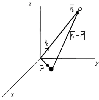
superimpose the fields radiated from each of these point sources to find the total radiated field of an antenna. Fig. 4.1 shows an antenna element location indicated by the vector r' and an observation location ro in the Fraunhofer farfield region, with ro representing the

unit vector along this direction. The distance between the source and point of observation is ro - r-. The radiation field U(ro) (either E or H field) due to this single isotropic

source is given in (4.1), where k = (commonly called wavenumber) and V is a

proportionality constant [22]. For simplicity and clarity of exposition, we will suppress this constant throughout the remainder of this thesis.

1 exp(jk --j)

U(r) = V (4.1)

Y

Fig. 4.1. Diagram of a single antenna element located at r' and a point of observation in the farfield at ro .

Superimposing the fields due to each of the elements along an aperture surface S, we find the total radiated field at a point of observation ro in the farfield of the aperture

antenna given by (4.2).

1

exp klro -j)

U(ro) = -ds

jA

With the farfield radiation approximation, - r r - 0 r, (kr 0 >> 1),

and assuming that the distance from each point on the aperture to the point of observation

1 1

is approximately equal outside of the exponent, - = -, this field expression

ro -ro -r ro

1 exp(jkrr _o) Iexp(-jki•r')ds

U(ro) = exp(-jko -r

jA

r

s

Since the antenna aperture we consider is a ring, it is more natural to express the field expression in spherical coordinates. We use standard spherical coordinate notation

z

as shown in Fig. 4.2. For a ring aperture with radius R on the x-y plane with 0'= -, the 2 radiated field expressed in spherical coordinates is given by (4.4), where we have used the equality r0 r' = R sin 90 cos(f'-o 0).

U(do, 0

o,0

)

d = x2 +2

[ sin cosos

r = r sin9sin ~

Scos

j

4.2 Radiated Power and Directive Gain

In Chapter 3, we discussed the impact of radiated power on the user data rate. From the field equation in (4.4), the total time-averaged radiated power from an individual transmitting aperture can be shown to be (4.5) [20]. Moreover, the radiated power in the desired direction and in the direction of interfering users will determine the

signal gain and interference levels in the network. The directive gain, or simply gain,

radiated power over 4z steradians (4.6) [20]. The maximum directive gain is called

directivity, denoted by D (4.7). We will make extensive use of these expressions in our

beamforming analysis in subsequent chapters.

Prad = II U(d, 0,)2 d 2 sin Od/dO

00

(4.5)

(

=U(d,

)

-Ya

4d

4)lU(d,

0,

)

f

0,0)1

sin

O&dlOd

00

Directivity = D = G(O, ) max

(4.6)

Chapter

5

Aperture and Array Beamforming

In this chapter, we present expressions describing the fields radiated by antenna apertures and arrays with beamforming. First, we consider the scenario where a single transmitter, utilizing conventional beamforming, transmits to a single receiver with a constraint of maximum average radiated power. We then note the symmetry in receive antenna beamforming and describe the maximum signal gain on an individual wireless link with conventional beamforming utilized on both the transmitting and receiving ends. Next, we extend the beamforming analysis to the case where a single multiple element antenna transmits different information, possibly at different power levels, to spatially distributed users. Finally, we outline the corresponding power allocation problem for the case where multiple users transmit and receive simultaneously in an infrastructureless wireless network.

5.1 Continuous Aperture Beamforming

We first focus on antenna beamforming for a ring aperture of radius R, centered at the origin of the x-y plane, transmitting a signal to a user located at (do, ,• 0). The

signal radiated from each point on the antenna is multiplied by a complex weight that varies with 0' along the ring aperture. The complex weight at the antenna, w(b'), can be written as:

w(6') = a, exp(jVy( '))

where ac is a constant with the subscript 'c' denoting a continuous aperture, and V/(z') is a complex phase term that is a function of b'. With this complex weighting, the radiated

aperture field at (do, 0, o0) becomes:

U 1 exp( jkdo) 2 w(') exp(- jkR sin 0_o cos(q'-~o))Rdo'

C°

acR

exp(jkdo)

y('))exp(- jkR sin 00 cos(b'-

))dz'

The phase function, V( '), ensuring that the product of exponentials in (5.2) is equal to one for all 0' and, therefore, maximizing the radiated field at (do,, 00), is

/l(q') = kR sin 90 cos(¢'-o0) (5.3)

This function serves to counter the effects of spatial delays to ensure that the fields radiating from all points on the aperture arrive at the desired location in phase. With this phase, we have the conventional beamforming weights for a ring aperture and radiated field at any point of observation in the farfield, (d, 9,), given by (5.4) and (5.5), respectively.

w(O') = acexp(jkR sin 80 cos(b'-• 0))

U(d, 0, ) =j acR exp(jkd) 2 exp(jkR sin 0_o cos( s'-₀o))exp(- jkR sin 0 cos(f'-O))do'

jA d 0

(5.5)

The amplitude ac is limited by the maximum average power constraint. Assuming the signal to be transmitted has unit amplitude, the total time-averaged radiated power of the antenna, from (4.5), is

D2 2f-2x]2g 2

Prad = a 22 exp(jkR sin 80 cos('-~₀o))exp(- jkR sin 0 cos(Qf'-))d sin Odqd0 2 R2 f2

=aZ 0 0Fe (0' )1 2 sin

Od(dO

(5.6)

where F, (0, ) is the array factor for a continuous aperture (5.7).

2Fx

FC (0, 0) = Jexp(jkR sin 00 cos('-~bo))exp(- jkR sin 0 cos(b'- ))dq'

0

(5.7)

Given the average power constraint Prad P,,, ac is upper bounded as

a 2 c -Ptot A 2 2K2P R 2 fF,r(0)2 Sin2 Oddr 00

(5.8)

With the complex weights described in (5.4) and the corresponding continuous array factor in (5.7), the achievable directivity (4.7) utilizing conventional beamforming on an aperture is

4a[U(do,9

,Bo)

Aperture 21r2R2

fI

U(d, O,

)j

_sin

_O&d

00

= 4lF (00 9 0

)1

(5.9)

f ýFC

(0, )12

Od6dlO

f ý'C(

*,

sin

00

As is evident in (5.9), the directivity does not have a simple closed form expression. We will later use Matlab to numerically calculate this directivity and then compare the results to that of an N-element array. We will now present the radiated field of a discrete antenna array with conventional beamforming, under the same transmit power constraint.

5.2

Multiple Element Array Beamforming

With the model of antenna elements as infinitesimal isotropically radiating point sources, an array is simply an aperture sampled with spatial impulses. The total field at a point of observation in the farfield is then a sum of the field from each of the discrete

antenna array elements. For an N-element UCAA with elements spaced uniformly along a ring of radius R, the transmit antenna array field at (do ,Oo, o) under conventional beamforming is

1 exp(jkdo) N-I

U(do,00'B,) = 1 do Iw(q', )exp(- jkRsinO° cos( 'n-00))

jA do n=O _(5.10)

(5.10)

a d exp(jkdo) N-1

= ad exp(jkdo) _{exp(jki(¢',, ))exp( jkR sin O0 cos(',} -00))

jAz do n-O

where w(',,) = ad exp(jGy(',, )) (5.11)

2nn

and ', = . The subscript 'd' on the amplitude of the complex beamforming weight, N

w(O', ), at the nth antenna array element, denotes a discrete array.

The main difference between conventional beamforming with a continuous aperture versus a discrete array is that an array can only adjust the signal phase and amplitude across the antenna at the set of finite, discrete sampled locations. The phase,

/( ', ), that maximizes the radiated field at (d0,00,o 0) by ensuring that the product of

exponentials has maximum value of one for all of the terms in the summation, is

g(0 ',1 ) = kR sin O, cos(',n -A0) (5.12)

With this phase, the radiated field from a transmitting antenna array with conventional beamforming, evaluated at any location in the farfield, (d, 0, 0), is

U(d,9,) exp(jkd) exp(kR sin 0 cos(', - 0))exp(- jkR sin 9 cos(q', -0))

jA d n=O

(5.13)

Recall that, under conventional beamforming, the amplitude ad is uniform across all of the elements. Thus, each array element transmits an equal fraction of the total power, which is limited.

Specifically, the total radiated power from the antenna array must satisfy the same power constraint as in the case of a transmitting aperture, namely Prad Po,. From (4.5),

the total radiated power for the antenna array is

2r2fx

Prad = jU(d,9, q)2 d2 sin OddO

= a2 - exp(jkR sin 90 cos(O' --o))exp(- jkR sinG cos(' -0) sin d

dO1

2 2x2xn

a•

JF

(0,

¢)I

sin d•4O

00

(5.14)

The quantity inside the absolute value in (5.14) is the discrete array factor, Fd (5.15).

N-i

Fd (0,

0)

Applying the power constraint on the transmitting antenna, we see that the array field amplitude, ad, must satisfy (5.16).

0 0

From (4.7) and with the discrete array factor in (5.15), the achievable antenna array directivity under the conventional beamforming scheme described by (5.11) is

4 lU(do,,o,

o)

DArray 2r2x

Jf

|U(d,

9,

)1

_sin

00

r

(

_(5.17)

d

•F , O12 sin dodO

00

4;dV2

2•S

Fd

00

Like the aperture directivity in (5.9), the expression for the circular array directivity in (5.17) also has no simple closed form. We will now show calculations of the array directivity from Matlab and compare the results to that of an aperture. Note from the previous discussion on spatial sampling of an aperture, we expect that, with increasing number of antenna elements, the radiated array field should approach that of

5.2.1 UCAA Directivity

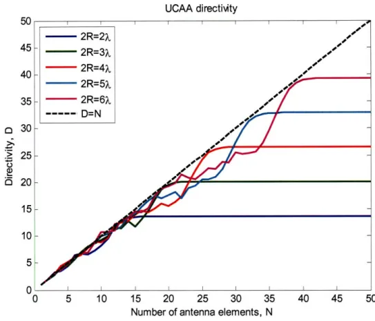
In Fig. 5.1., we plot the array directivity (5.17) for UCAAs of different diameters as a function of the number of antenna elements N. First, note that the array directivity for a given antenna size and carrier wavelength remains constant when increasing N beyond a certain point, Nsat. Thus, in the limit as the number of elements approaches infinity, the aperture directivity is the same as that of an array with "large enough" element density. Moreover, examining the curves in Fig 5.1, we find that the UCAA directivity is approximately proportional to N up to a point. In the following discussion, we will determine the number of elements, Nsat, beyond which the array directivity remains constant.

UCAA directivity

0 5 10 15 20 25 30 35 40 4 0

Number of antenna elements, N

Fig. 5.1. UCAA Directivity versus the number of antenna elements for different antenna sizes.

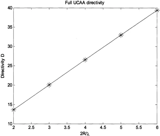
In Fig. 5.2, we plot the maximum directivity of each curve in Fig. 5.1 as a function of the ratio of the array diameter, 2R, to transmit wavelength 2.

--Full UCAA directiity

2 2.5 3 3.5 4 4.5 5 5.5 6

2R/X

Fig. 5.2. Maximum Array Directivity as a function of the ratio of antenna size to carrier

wavelength, 2R/, . The '*' represents computed directivity for the different ratios.

From this figure, we see that the maximum achievable directivity of a UCAA is approximately linearly proportional to the ratio 2R

_A.

2R

directivity is approximately 21r times the ratio A. From this analysis of maximum

4 rR

directivity, we find that N, is proportional to 4d?. Since N, must necessarily be an integer, we approximate this point of saturation as

--Nsat - = (5.18)

S

A (A / 2)

From (5.18), we see that the integer N sat corresponds to element spacing of

approximately )/2 along the array circumference, 2zR. From a sampling standpoint, Nsat is the number of UCAA elements required to sample the corresponding ring aperture at the spatial Nyquist sampling rate [21]. With this approximation in (5.18) and noting from Fig. 5.1 that the array directivity is approximately linear with N up to the point of saturation, Nsat , we have the array directivity DArray:

N, for N < Nsat

DArray for sat (5.19)

Nsat , otherwise

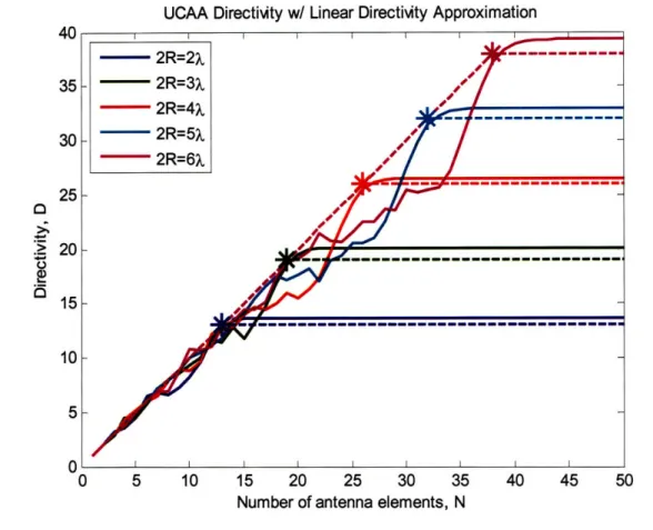
Fig. 5.3 plots the UCAA directivity for the same parameters plotted in Fig. 5.1, with our linear approximation (5.19) shown with dashed lines, and with the values of

Nsat from (5.18) indicated by a star (*). From this figure, we see that our approximation to the UCAA directivity closely follows the calculated curves in Fig. 5.1.

UCAA Directivity w/ Linear Directivity Approximation 30 25 20 15 10 0 5 10 15 20 25 30 35 40 45 50

Number of antenna elements, N

Fig. 5.3. Calculated UCAA directivity (5.17, solid), with linear approximation (5.19,

dashed). Nsat indicated with a star '*'.

Since the array directivity is approximately proportional to the number of array elements, it takes on integer values in (5.19). A continuous aperture, on the other hand, does not have a discrete, integer number of elements. Thus, we can approximate DAperture directly as

(5.20)

D e _{Aperture -}r

/

Fig. 5.4 plots the maximum achievable directivity as a function

of

,

as seen in

AZ

Fig. 5.2, with the approximation to Nsat in (5.19) shown in red and the aperture 2R=2X 2R=3X 2R=4X - 2R=56 ---2R=56 I I I I I I I I I

m

-Zr

t

k

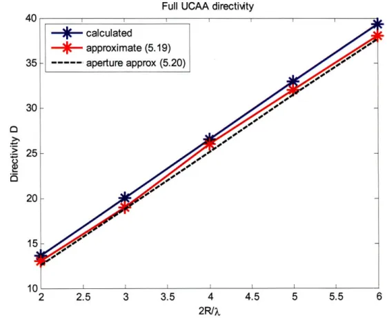
directivity approximation (5.20) in black. In Fig. 5.4 and Fig. 5.5, we see that our approximations to the UCAA directivity and points of saturation closely follow the calculated trends. We will use these approximations throughout the remainder of this thesis in order to simplify the integral equations in the previous section, allowing us to later offer insight into the behavior of data rates in the network without extensive calculations and simulations.

Full UCAA directivity

2 2.5 3 3.5 4 4.5 5 5.5 6

2R/X

Fig. 5.4. Maximum UCAA directivity, calculated (blue) and approximated (red) as a function of the ratio of antenna size to carrier wavelength, 2R/2A. Our approximation to

5.2.2 Aperture & Array Beamforming Revisited

Following the directivity analysis in Matlab, we can now revisit aperture and array beamforming using our approximations in (5.18)-(5.20). With the array directivity in (5.19) that is proportional to N, the denominator in (5.17) becomes 4rN for N • Nsat

J

Fd

(,')I

&Wdo

=

4NdV

(5.21)

00

Similarly, from (5.20), the denominator in (5.9) is given by

f2F,(,•F (0)12 sin &Id0

=

_(5.22)

00R

Using these values in (5.21) and (5.22), from (5.8) and (5.16), the maximum amplitudes on the aperture and array transmit fields, a, and ad, that satisfy the power constraint are:

ac ot (5.23)

a--:

ad 2 (5.24)

otherwise

The user receive power will be determined by

IU(do,

o)I

.

analysis of the directivity and complex weights of a UCAA utilizing conventional beamforming, this is equal to

tot R DAPerturetot

- - 2 ,ZdAperture d2 A 4d2

NPo, DArray Pot (5.25)

o 4yo' r Array

4nd2

4d2Array

Note that, in terms of the aperture and array directivities defined in (5.19) and (5.20), the final expressions for the magnitude squared receive field due to a transmitting aperture and array are equivalent.

5.3 Receive Beamforming

Up to this point in this chapter, we have focused on beamforming for a transmitting aperture and array. We will now describe the dual receive beamforming problem. Recall that we are operating under a far-field assumption, so that the transmitted field at the receive aperture or array is well approximated by a plane wave. For the receive beamforming analysis, consider a circular antenna centered at the origin. Let this circular antenna now receive an incoming plane wave from a transmitting user located at

(do,

o,

o) .

On the receive end, the plane wave signal arriving at the antenna elements is scaled by complex beamforming weights and then summed to get the overall receive

power. From [21], the complex phase on a receiving antenna array, r,(Z',), that

maximizes the receive power from a user transmitting at (do, 00, o) is given by

y/, (', ) = -kR sin 00 cos(b', - 0o) = -V( ', ) (5.26)

From (5.26), we see that the transmit and receive beamforming problems are symmetrical.

Unlike transmit antenna beamforming, the amplitude of the complex receive beamforming weights is not limited by the constraint on total time-averaged radiated power. In this thesis, we choose to normalize the receive beam, as in [21], such that the maximum receive gain is one and the gain in all other directions is less than unity. Thus,

1

the amplitude on the receiving antenna array elements is . Given this amplitude and

N

the phase in (5.24), the complex weight, w, (0',), on the nt_{h element of a UCAA under a} conventional beamforming scheme is given by (5.27).

w, (',n ) = - exp(- jkR sin 9O cos(', -~0)) (5.27)

N

Now that we have described conventional beamforming on both the transmitting and receiving ends of a single wireless link, we can extend our results to the case of transmitting simultaneously to multiple users from an individual antenna array.

5.4

Beamforming & Power Allocation for Multiple User

Transmissions

Before considering beamforming and power allocation for simultaneous transmissions from a single antenna to M-1 users, we first outline the assumptions on the user signals sent over the wireless links. The information transmitted in the infrastructureless wireless network lies in the time-varying waveforms that each antenna element transmits. The signal transmitted to user j is the time-varying waveform vj(t). Following the discussion of the user signals in [1], we assume that the user signals vj(t) are independent of each other and their individual time-averaged value, vj(t), is zero

(5.28) but the time-averaged magnitude squared of each signal, Ivj (t) , is unity (5.29).

vj(t) = 0 (5.28)

Iv

(t

l

= 1

(5.29)

Furthermore, we assume that different user signals are uncorrelated:

v, (t)v' (t) = 0, k # j (5.30)

With these assumptions on user signals at the transmit antenna array, we can superimpose multiple beams directed towards spatially distributed users. More specifically, given these signal properties, the beams for distinct user signals will not distort each other and the amplitude and phase at the antenna elements decouple for different user transmissions. Thus, beamforming for multiple simultaneous user

transmissions at a single antenna array is simply a superposition of the beams formed for each user transmission. Moreover, due to the assumption that user signals are uncorrelated, the total radiated power is the sum of the power radiated by each of these beams, which is constrained by the limitation on total time-averaged transmit power from an individual antenna.

At an individual antenna array element, each user transmission is given a distinct complex weight. The complex weights for each of the M-1 simultaneous user transmissions are determined by (5.12). The amplitude on each set of complex weights is determined to satisfy the overall power constraint. That is, each user transmission is allocated a fraction aj of the total available power, Ptot, at an individual antenna, where

0 < ac < 1. Hence, the sum of all of the a. terms for M -1 user transmissions from a

single antenna must be less than or equal to one (5.31).

M-1

aj <1 (5.31)

j=1

With this power allocation scheme, the limitation on power for each individual transmission from a particular antenna becomes ajPt .From (5.22), the corresponding amplitude on the complex antenna array element weights for a particular user

transmission is then

a. = t _(5.32)

With this amplitude, the magnitude squared of field received at user j, located at

(do, ,•o ), from an individual transmitting antenna is

(do o)2 N P t DArray aj Ptot

U4(d0o

For a network of M wireless users, the power allocation scheme described above is applied at each transmitting user antenna. The fraction of total power allocated by user

i to a transmission to user j, aij, will determine the receive power at user j on this individual link. With normalized maximum receive gain, the receive power at userj due to a transmission from user i is then

= NaPtot (5.34)

P"

On the other hand, the power allocated to other wireless links will determine the levels of interference received at user j. From (3.1), we see that the achievable data rate on a wireless link formed by user i transmitting to user j is determined by the receive power and interference at user j. Thus, the a 's in the power allocation scheme for the network will determine the achievable data rates.

The power allocation scheme described above can be summarized for the entire wireless network in the power allocation matrix shown in (5.35). Each ai. term in the

user j. The diagonal in the power allocation matrix is zero to indicate that there are no self-transmissions. Also, from (5.29), the sum of the entries in each row of the power allocation matrix must be less than or equal to one.

Power Allocation Matrix

0 a₁2 a13 aIM

a₂₁ 0 a23

a31 a32 0

•a•M 0

(5.35)

As discussed above, the power allocation scheme specified by the matrix shown in Fig. 5.5 will determine the achievable data rates on individual wireless links in the network. The problem of joint beamforming and power allocation to achieve a desired traffic pattern in a network considers solving for the a 's in the matrix above in order to satisfy the user data rate demands. Due to the interference terms that link the power allocation and achievable data rates for different users, determining the power allocation scheme to satisfy a given traffic pattern for a network with a large number of users can be difficult. To get a sense of the network problem, we will consider power allocation and examine achievable data rates for a simple network of three users.

Chapter 6

Beam Characteristics, Sidelobe Behavior, and

Interference in the Wireless Network

Multiple simultaneous transmissions, as discussed in Chapter 5, cause interference in a wireless network. The amount of interference at a user is determined by the amount of power allocated to interfering transmissions and the transmit and receive gains between user pairs. In Chapter 5, we examined the maximum directive gain of a beam formed by conventional beamforming at a UCAA. In order to find the amount of interference at a user, we need to examine the directive gain of an antenna in all directions. This chapter will focus on the beampattern of a UCAA in order to characterize the mutual interferences of multiple transmissions in an infrastructureless wireless network.

6.1 Beampattern and Beamwidth

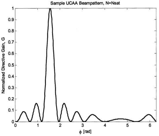
Since the users in our wireless problem transmit and receive on the x-y plane (i.e. 0 = r/2 ), we are only concerned with the antenna directive gain as a function of b. An

example beampattem for a UCAA with radius R = 2 and N,a, elements is shown in Fig.

6.1, which plots the directive gains (normalized by the directivity) versus

0.

• = - direction. The beam pointing in the 40 direction is called the mainbeam. Outside

of the mainbeam, there are sidelobes and nulls. Sidelobes are the secondary peaks and nulls are points at which the directive gains are zero.

Sample UCAA Beampattem, N=Nsat

1 2 3 4 5 6

0 [rad]

Fig. 6.1. Beampattern for a UCAA of radius R = 2 with Nsa, elements.

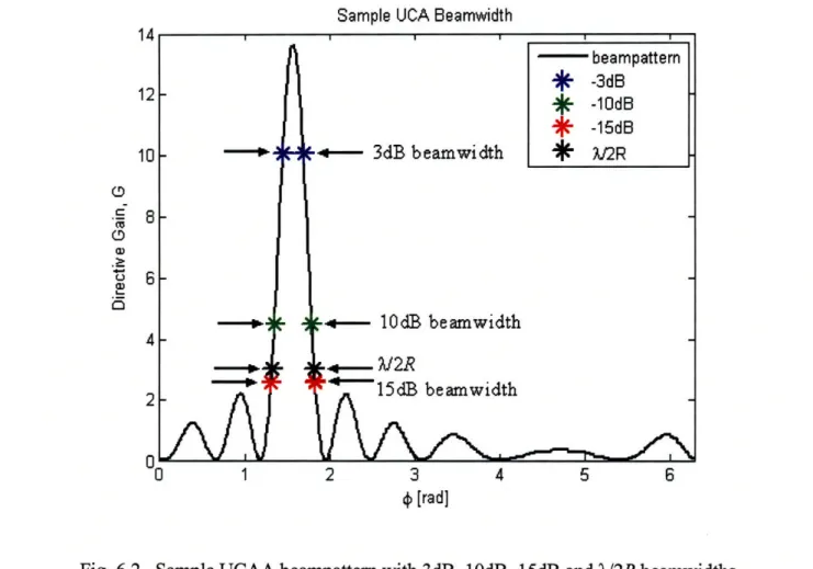
An important parameter in characterizing the mainbeam is the beamwidth. This angular beam width is typically measured between points along the mainbeam that are 3dB lower than the directivity, as shown in Fig. 6.2. One can also define the beamwidth by other dB values such as 10dB or 15dB as indicated by Fig. 6.2. The beamwidth is proportional to and, subsequently, we will take the mainbeam width to be 2/2R [19].

2R 1 0.9 0.8 0.7 0.6 0.5 0.4 0.3 0.2 0.1 0

Sample UCA Beamwidth

0 1 2 3 4 5 6

4 [rad]

UCA Beamwidth U.5 U 0.5 0.45 0.4 0.35 o 0.3 E 0 0.25 0.2 0.15 0.1 0 05 2 2.5 3 3.5 4 4.5 5 5.5 6 2R/l

Fig. 6.3. UCAA beamwidth as a function of the ratio of antenna diameters to carrier wavelength, 2R/A,.

Fig. 6.4 shows polar plots of the beampattern for two different arrays with different diameters. In these plots, as expected, the mainbeam beamwidth is smaller for the larger array, indicating that larger arrays can focus more power in the desired direction. In general, the beampattern of an antenna depends not only on the antenna diameter, but also on the number of antenna elements as we will show next.

Normalized UC• Beampattem / - t L 1 0.80.0 0 ' -2_ -/2 - 3 2R/X=2 Normalized UC Beampattem

2

3

1

_{0. 0. 0.}

-d2

Fig. 6.4. Comparison ofUCAA beamwidths for two different ratios of antenna diameter

to carrier wavelength (normalized polar beam plots).

6.2 Spatial Aliasing in the UCAA Beampattern

Recall from Chapter 5 that the UCAA directivity does not change for N > N,,,. Similarly, from our study in Matlab, we find that the beampattem does not change significantly for N > N,at,,. Consequently, in the remainder of this chapter we consider

UCAAs with N 5 Nsa, elements.

A UCAA with N < Nsat elements is spatially sampled below the Nyquist rate (i.e. undersampled) which causes spatial aliasing in the UCAA beampattern. That is, the beampattern for an under-sampled UCAA will contain grating lobes, or spatially aliased sidelobes. Fig. 6.5 shows polar plots of the beampatterns of a UCAA with radius R = A

N=1 _N=2

N=3 _N=5

N=7 _N=9

0

-d2

N=11 N=13 (full array)

Fig. 6.5. Polar beam plots: Nsa, = 13,2R/A = 2, 0 =

-2

Comparing the spatially aliased beampatterns in Fig. 6.5 to that of a "full" array in the last plot of Fig. 6.5, we note that the sidelobes in the beampattern for a full array are much lower than the grating lobes of the under-sampled UCAAs. Moreover, as is evident in Fig. 6.1, the sidelobes for a full array decay in amplitude with increasing angle away from the mainbeam, whereas the grating lobes do not always decrease.

To see the variability in grating lobe locations for a range of under-sampled arrays, we plot the beampattern for a UCAA of radius 3A as a function of N and 0 in Fig.

6.6. We see that the directivity of these arrays (in o = - direction) grows linearly with

2

N and saturates at N = Nsa,, as described in Chapter 5. Outside of the mainbeams, we observe grating lobes that vary significantly in amplitude and location as a function of N and 0. These properties of grating lobes for UCAAs indicate that the interference gains in a network can vary significantly with user location and number of antenna elements N.

Beameettemr vs N, 2RbA6 : : '36, 30, 0-, 5.

N

[rad]

Fig. 6.6. UCAA beampattem as a function ofN, Nsa, = 40, 2R/A = 6, 0 = ₂

6.3 Sidelobe levels of a UCAA Beampattern

The sidelobe levels of the antenna transmit and receive beams will determine the amount of interference that users in a network will experience. Consequently, the precise level of interference at a receiver depends on the exact user locations. Calculation of these interference levels directly from (4.7), for each possible user location, is computationally intensive, particularly, if the nodes are not static. Meaningful analysis of the wireless channels therefore requires some simplification and parameterization of the sidelobes and, correspondingly, interference levels. For our goal of gaining insight into the achievable data rates of infrastructureless wireless networks, we make

Jn

~ i "

··· ·i·IIi'i: r·iii t 1 i

approximations to the sidelobe levels in order to find an expression for the data rate on an individual wireless link that is independent of the precise user locations. Specifically, we determine the minimum, maximum and average sidelobe levels of a UCAA as a function of the density of antenna array elements in order to provide insight into the best, worst and average performances in the infrastructureless network, respectively.

In particular, we define the maximum (minimum respectively) sidelobe level as the ratio of the maximum (minimum respectively) gain outside of the mainbeam to the directivity. Similarly, the average sidelobe level is the ratio of the average value of the sidelobes to the directivity. To find the average value of the sidelobes, we integrate the beampattern outside of the mainbeam (specified by the beamwidth ) and divide by

2R

2z; 2. We will express the sidelobe levels as a fraction, ý, that lies between zero, for a 2R

null, and one, corresponding to the directivity. Moreover, we express C as a function of

N/ Nsa,,,, a term that indicates the density of antenna elements, or sparsity of the array.

6.3.1 Maximum Sidelobe Level

The maximum sidelobe level describes the largest gain on interfering transmissions and therefore captures the worst case performance in the wireless network. We attempt to find a curve that envelopes most of the UCAA maximum sidelobe levels

as a function of N/Nsa,. From numerical computation, we find that .max is 0.16 for N = Nsa,,,, as shown in the beampattern for a full array in Fig. 6.1. With this observation and

examination of the UCAA maximum sidelobe levels in Matlab, we make the approximation to the UCAA maximum sidelobe level, Cm:

(' =1.16 - N/,t (6.1)

Fig. 6.7 plots the maximum sidelobe level of beampatterns of UCAAs of different relative sizes as a function of N/N,,t. Our enveloping approximation to the UCAA

maximum sidelobe level is shown on this plot in black and, as is evident in Fig 6.7, captures the trends of the maximum sidelobe levels.

Max Sidelobe -to- Peak Ratio, ýmax=-(1/Nsat)*N+1.16 1.1 0.9 0.8 0.7 0.6 0.5 0.4 0.3 0.2 al 0 0.2 0.4 0.6 0.8 1

Array Sparsity, N/Nsat

Fig. 6.7. Ratio of Maximum Sidelobe-to-Peak UCAA beam level as a function of array sparsity N Ns , shown with the approximation

'x

To see the individual curves in Fig. 6.7 more clearly, we show plots of the calculated (blue) and approximate (green) maximum sidelobe levels in Fig. 6.8 for each relative UCAA size. As is evident in Fig. 6.8, our approximation, m7x, lies on the calculated curves for smaller UCAAs and envelopes, or offers a more conservative estimate, of the sidelobe levels for larger UCAAs.