Algorithms for Data Mining
by
Grant J. Wang
B.S., Computer Science, Cornell University 2001.
M.S., Computer Science, Massachusetts Institute of Technology 2003.
Submitted to the Department of Electrical Engineering and Computer
Science
in Partial Fulfillment of the Requirements for the Degree of
Doctor of Philosophy in Electrical Engineering and Computer Science
at the Massachusetts Institute of Technology
September 2006
@ MMVI Massachusetts Institute of Technology. All rights reserved.
The author hereby grants to M.I.T. permission to reproduce and
distribute publicly paper and electronic copies of this thesis
and to grant others the rigto
g1q
so.Author ... .. .... .. ...
Department of Electrical Engineering and
mputer Science
August 8, 2006
C ertified b y ...
...
Santosh Vempala
Associate Professor of Mathematics
Ti
Supervisor
Accepted by ... g ... .. ..
Arthur C. Smith
Chairman, Department Committee on Graduate Theses
OF TECHNOLOGY
Algorithms for Data Mining by
Grant J. Wang Submitted to the
Department of Electrical Engineering and Computer Science on August 8, 2006
In Partial Fulfillment of the Requirements for the Degree of Doctor of Philosophy in Electrical Engineering and Computer Science
ABSTRACT
Data of massive size are now available in a wide variety of fields and come with great promise. In theory, these massive data sets allow data mining and exploration on a scale previously unimaginable. However, in practice, it can be difficult to apply classic data mining techniques to such massive data sets due to their sheer size.
In this thesis, we study three algorithmic problems in data mining with considera-tion to the analysis of massive data sets. Our work is both theoretical and experimental - we design algorithms and prove guarantees for their performance and also give ex-perimental results on real data sets. The three problems we study are: 1) finding a matrix of low rank that approximates a given matrix, 2) clustering high-dimensional points into subsets whose points lie in the same subspace, and 3) clustering objects by pairwise similarities/distances.
Thesis Supervisor: Santosh Vempala Title: Associate Professor of Mathematics
Acknowledgments
I thank Santosh. I remember when I first scheduled a meeting with Santosh five years ago. Unlike other first year graduate students, I was without a research advisor. Much of that first semester was spent worrying about whether I'd ever get an advisor. Enter Santosh, who was immediately willing to begin scheduling weekly meetings with me. At the time, I thought it was wonderful, but it's only now that I realize how incredibly lucky I was. Santosh has always believed in my ability to produce good work, even if I didn't believe it myself. Halfway through my time at MIT, I was thinking about leaving. I'm glad that he convinced me against this. I have really learned how worthy it is to keep at something, even though things may not seem so rosy in the moment. I really also appreciate his interest in my research later in my graduate career, as I began to work on more applied things. Without his input, the quality of my work would have been far worse.
I thank Lillian Lee and Andrew Myers. As my interest in computer science was peaking, I took CS481 at Cornell with Lillian. I had never been gripped so much by a subject as I was by the theory of computation. I very much appreciate the interest she showed in me whenever I came by her office to talk about graduate school. Andrew gave me my first research experience, and I thank him for taking time out to supervise a bunch of undergraduates. Without professors believing in me as an undergraduate,
I would have never thought I could go on and get a PhD.
I have been blessed with amazing friends. I thank my very good friends from high
school. AJ, Dan, Dermot, Matt, Matt, Mike, and Will - it's been almost 10 years since
we graduated high school. When I read this ten or twenty years down the road, it will make my heart warm that I didn't need to write down your last names. Our friendship (and our fantasy football league) will still be alive and kicking. A special thanks goes
out to AJ and Matt. AJ - besides being an unbelievable friend, I want to say thanks
for introducing me to my entire social circle. You have great taste in people. Matt
-you have been such a great escape from proving theorems and running experiments. Thanks for all the McDonald's runs and Sunday trivia nights. I've been so lucky to
have someone I grew up with here in Boston with me. Wing - thanks for cooking all
those dinners for me, giving me rides, spotting me money, etc. You may not realize it,
but you have taught me a great deal about life. Jen, Jess, and Cy - I've spent so much
of my social time with you these past few years, and it's been wonderful. I regret that
I didn't have more time to just hang out with all of you.
Mom, Dad, and Leslie - I love you all very much. Thanks for all the support and the phone calls. We've all lived in different areas and it's been hard to stay in touch with my busy schedule. I appreciate all the understanding you've given me when I haven't wanted to talk. I'm glad we'll all be in California together soon.
Feng. We started dating a little more than two years ago when school was really tough for me. You've been there with me through all of this. Even in my darkest times, you've always somehow found a way to bring a smile to my face. I realize that
when I've been most stressed I haven't exactly been the easiest to get along with - at
I admire and respect you so much for that. You've come so far and you have no idea
how proud I am of you. When you landed a great career opportunity in California, I never had any doubt in my mind that we'd be anywhere else. I want to spend the rest of my life with you. Feng, will you marry me?
Grant Wang Cambridge, MA
Contents
1 Introduction 7
1.1 Low rank matrix approximation . . . . 8
1.1.1 Our work . . . . 10
1.2 Projective clustering . . . . 11
1.2.1 Our work . . . . 13
1.3 Clustering by pairwise similarities/distances . . . . 14
1.3.1 Our work . . . . 15
1.4 Organization of this thesis . . . . 16
1.5 Bibliographic Notes . . . . ... . . . . 16
2 Preliminaries and Notation 17 2.1 Probability, random variables, and expectation . . . . 17
2.2 Linear algebra . . . . 17
2.2.1 Singular Value Decomposition . . . . 18
3 Low Rank Matrix Approximation 21 3.1 Introduction . . . . 21
3.1.1 Motivation . . . . 21
3.1.2 Our work . . . . 23
3.2 Improved Approximation for Low-Rank Matrix Approximation . . . . . 25
3.2.1 Related work . . . . 25
3.2.2 Adaptive sampling . . . . 26
3.2.3 Relative approximation . . . . 30
3.2.4 N otes . . . . 31
3.3 Benefit of Spectral Projection for Document Clustering . . . . 32
3.3.1 Related work . . . . 32
3.3.2 Approximation . . . . 32
3.3.3 Distinguishability . . . . 35
3.3.4 Notes and Further Questions . . . . 39
4 Projective Clustering 40 4.1 Introduction . . . . 40
4.1.1 Motivation . . . . 40
4.2 Related work . . . . 41
4.3 Intuition and a factor k + 1 approximation algorithm . . . . 42
4.4 Polynomial time approximation scheme . . . . 44
4.5 Analysis of the 6-net . . . . 45
4.6 Correctness of the algorithm . . . . 47
4.7 N otes . . . . 49
4.8 Further questions . . . . 49
5 Divide-and-Merge methodology for Clustering 50 5.1 Introduction . . . . 50
5.1.1 Background and Motivation . . . . 50
5.1.2 O ur work . . . . 52
5.2 Divide-and-Merge methodology . . . . 53
5.2.1 A spectral algorithm for the divide phase . . . . 54
5.2.2 Merge phase . . . . 60
5.3 Application to structuring web searches: EigenCluster . . . . 62
5.4 Comparative experiments on standard data sets . . . . 64
5.4.1 Comparative measures . . . . 64
5.4.2 Spectral algorithm as the divide phase . . . . 67
5.4.3 Merge phase in practice . . . . 73
5.5 Predicting health care costs . . . . 75
5.5.1 Data, Measures, and Experimental Setup . . . . 75
5.5.2 Prediction Algorithm . . . . 76
5.5.3 R esults . . . . 77
Chapter 1
Introduction
Data of massive size are now available to researchers in a variety of fields such as biology (microarray and genetic data), sociology (social networks data), and ecology (sensor network data). These data sets come with great promise. Vast amounts of useful information such as gene interactions in biology, patterns of social interaction in sociology, and small-scale environment dynamics in ecology are said to lie in the data. The goal of data mining is to extract this useful information [HK01, HMS01].
A key challenge in data mining is that the useful information we wish to extract is not known beforehand. For this reason, basic tools such as dimension reduction and clustering play a central role in data mining. In general, these tools aid data exploration, a first step to extracting useful information from data. Many data sets can be described as an n x m matrix, where n is the number of objects in the data set, and m is the number of features that describe each object. Dimension reduction refers to the technique of decreasing the number of features from m to some p
<
m. Withfewer features, it can be easier to detect underlying structure in the data. Indeed, in some circumstances, dimension reduction can even highlight the underlying structure. By representing the data in less space, data mining algorithms can be applied more efficiently. Clustering, the task of grouping together similar objects in a data set, also aids data exploration. The output of clustering is a set of clusters. Objects in clusters are similar, whereas objects from different clusters are dissimilar. Clustering is often a first step in extracting useful information because it gives a global view of the data set and how it naturally partitions. The uses of dimension reduction and clustering in data mining extend beyond just data exploration; for more uses, see [HKO1, HMS01].
While techniques for dimension reduction and clustering have been known for decades, massive data sets provide new challenges for these data mining tools. Al-gorithms for dimension reduction and clustering that run in polynomial time may no longer be considered efficient when applied to massive data sets. A more difficult prob-lem is that it may be impossible to blindly apply these algorithms. For instance, an algorithm may assume random access to data. However, massive data sets may not be able to be stored in main memory and the only access to such data may be through sequential reads (e.g. the data resides on tape). An additional problem massive data sets pose is that classical techniques may not even be relevant. For instance, most
classical clustering algorithms tend to be concerned with pairwise distances. Database researchers have found that in many real data sets, pairwise distance is a poor measure of the true "closeness" of points [AGGR05].
In this thesis, we study problems in dimension reduction and clustering with con-sideration to the data mining of massive data sets. Our work is both theoretical and experimental - we design algorithms and prove guarantees for their performance and also give experimental results on real data sets.
We focus on a particular technique for dimension reduction - low rank matrix ap-proximation. We develop a new algorithm for low rank matrix approximation with improved approximation when the data can only be accessed sequentially. Our al-gorithm gives a tradeoff between an additive approximation term and the number of sequential passes over the data. We also give an experimental explanation for why low rank matrix approximation is such an effective technique in information retrieval.
For clustering, we study two problems: projective clustering and clustering pairwise similarities/distances. Projective clustering is the problem of finding a partition of a high-dimensional point set into subsets so that points in the same subset lie in the same low-dimensional subspace. The problem was introduced by data-mining practitioners who discovered that traditional clustering algorithms such as k-means and hierarchical clustering perform poorly on real data sets with a large number of features. We give a polynomial-time approximation scheme for the projective clustering problem. For clus-tering pairwise similarities/distances, we introduce a divide-and-merge methodology. The methodology consists of a divide phase, in which a tree is formed by recursively partitioning the data, and a merge phase, in which an objective function is optimized over the tree to find a partition of the data. For the divide phase, we suggest a spectral algorithm with theoretical guarantees
[KVV04].
When the data take the form of a sparse object-feature matrix and similarity is defined to be the inner product between feature vectors, we give an efficient implementation that maintains the sparsity of the data. We also present a thorough experimental evaluation of the methodology on manyreal world data sets.
The rest of this chapter describes the use of low rank matrix approximation, pro-jective clustering, and clustering by pairwise similarities/distances in data mining and describes in more detail the contributions of this thesis.
1.1
Low rank matrix approximation
The best rank-k approximation of a matrix A
C
Rmxn is a matrix Ak E Rmxn suchthat |1A - AkJ|1 is minimized over all matrices of rank k. Geometrically, we can think
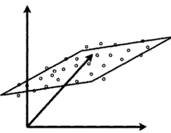
of low-rank matrix approximation as finding a "best-fit", low-dimensional space for A. Indeed, for k = 1, the problem corresponds to the well-known "best-fit" line for the data going through the origin, as in the Figure below. Here, the empty circle points are rows in the matrix A, and the filled circle points are the rows in the matrix Ak. The error of the approximation is the sum of the squared lengths of the gray arrows. In higher dimensions, the rows of A are points in R' and the rows of Ak are points in
c.A
Figure 1-1: Low rank matrix approximation for n = 2, k = 1
R" lying on some k-dimensional subspace.
The matrix Ak has found numerous applications. Perhaps the most immediate application is compression. When I A - Ak 11 is small, one can store Ak instead of
A. While A requires m x n space, Ak can be stored as m vectors in Rk along with k basis vectors that span the rowspace of Ak, requiring only m x k + n x k = k(m + n)
space. Indeed, low rank matrix approximation has been used for image compression [AP76, GDB95, WR96, YL95].
Ak can also be used to highlight the structure of A, thus aiding data mining tasks. This amazing property of low rank matrix approximations has seen numerous uses in areas such as information retrieval [DDL+90, BD095], collaborative filtering [SKKROO,
BP98, GRGP01], and learning of mixture models [AM05, KSV05, VWO4]. One area
where low rank matrix approximations have seen much use is the problem of document
clustering [Bol98, ZDG+01, DHZ+01, Dhi0l, ZK02, XLG03, LMOO4]. In this problem,
an algorithm is given a set of documents. The algorithm's task is to partition the set of documents so that each subset comprises documents about the same topics. Algorithms that cluster based on the low-rank matrix approximation of the document-term matrix of the document set are known as spectral algorithms. These spectral algorithms have shown impressive experimental results by correctly classifying document sets on which traditional clustering algorithms fail.
The wide use of low rank matrix approximation has motivated the search for faster algorithms for computing such approximations. The classical algorithms for computing
Ak compute the Singular Value Decomposition of a matrix, which we describe in more detail in Chapter 2. These algorithms are efficient in that they run in polynomial time -- O(min{mn2, nm2}). However, it may be infeasible to apply these algorithms
to massive data sets. Besides the running time being too long, the entire matrix may not fit into main memory. Motivated by these problems, researchers developed new algorithms for computing approximations of Ak [AMO1, FKV04, DKF+04]. The key idea in these algorithms is the use of random sampling. The algorithms apply classical
methods for computing low-rank matrix approximation to a judiciously chosen random sample of the original matrix. Since the random sample is much smaller than the original matrix, the amount of computation is much smaller. These algorithms based on random sampling offer the following guarantee: with constant probability, they output a matrix Ak such that
|A - AkH|' ;
I1A
- Ak||' +e\|AI|1.
At most two sequential passes over the data are required for random sampling. Thus, these algorithms can be useful when the data resides on tape and sequential passes are the only way to access the data.
Spectral clustering algorithms for document clustering [Bol98, ZDG+01, DHZ+01, Dhi0l, ZK02, XLG03, LMOO4] each use the low-rank matrix approximation of A in slightly different ways. The varied uses of spectral clustering algorithms in document clustering along with their common experimental success motivate the question: do the proposed spectral algorithm share a common benefit for document clustering? There has been both theoretical and experimental work attempting to explain the success of spectral methods. Theoretical work has focused on proposing generative models for data and showing that particular spectral algorithms perform well in the respective models [PRTVOO, AFK+01, KVV04, McSO1, VW04, KSV05]; An exception is the work of [KVV04] that gives a worst-case approximation guarantee for recursive spectral partitioning. Experimental work [DM01, SS97] has focused on slightly different dimension-reduction techniques or has explained the benefit of using low-rank matrix approximation with respect to a specific clustering algorithm.
1.1.1
Our work
We generalize the random sampling procedure in [FKV04] and provide a new algorithm for low rank matrix approximation. We also provide an experimental explanation for why spectral clustering algorithms are so successful in document clustering tasks.
Let us first recall the probability distribution over rows A( that is used in [FKV04]:
Pr (A(') is chosen) = .IAII1
Our generalization samples rows adaptively in many passes. In the first pass, we sample rows according to the distribution above, i.e. proportional to the squared length of the rows. In subsequent passes we modify the distribution. Let V be the subspace spanned by the rows we have already sampled. In the next pass, we sample rows proportional to their squared lengths orthogonal to V. In particular:
Pr (A(') is chosen) = (A('))I12 .1irv±
E 1 Ivi(A(3))12
'
Note that when V = {0}, this distribution is exactly the distribution used in [FKV04]. We call this generalization adaptive sampling. We show that if we sample adaptively in
t rounds, with constant probability there exists a rank-k matrix Ak lying in the span of all the samples such that:
1
||A
-Ak||
1
12||A - Ad 1| + E'I||AI|1.1 - F F
Thus, the additive error drops exponentially in the number of rounds. The intuition is that rows far from the span of the current sample incur large error. To ensure they do not continue to incur large error, we sample proportional to their error, i.e. their squared length orthogonal to the span of the current sample. This result gives rise to a randomized multipass algorithm. Combining adaptive sampling with volume sampling [DRVW06], we prove that there exists a subset of rows of A in whose span lies a relative (1 + E) approximation. To be precise, we prove that for every matrix A E R"', there exists a subset of k + k(k + 1)/c rows in whose span lies a rank-k matrix Ak such that:
hA - AkIF 5 (1 + e)IIA - Ad
F-This existence result proves useful for the projective clustering problem, which we study in Chapter 4.
We propose that the benefit of low-rank matrix approximation for spectral cluster-ing algorithms is based on two simple properties. We describe how these properties aid clustering and give experimental evidence for this. The first property is that low-rank matrix approximation is indeed a good approximation of the original matrix. By this, we mean that ||A - AkhI is sufficiently small, as compared to ||Ail. The second
property is that the true clustering becomes more apparent in the low-rank matrix ap-proximation. In particular, documents about the same topic lie closer to each other and documents about different topics lie farther away. We also discuss a connection between this second property and recent theoretical work on learning mixtures of distributions. Both of the two properties we suggest are independent of any specific algorithm.
1.2
Projective clustering
Projective clustering is the problem of partitioning a point set P C Rd so that each
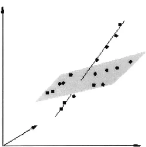
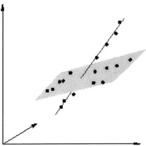
partition approximately lies in the same subspace. This problem differs from the classic problem of clustering points in which points from each partition are desired to be close to their centroid. For some data sets, points fail to cluster around center points, although significant structure still exists in the data set. For instance, the points in Figure 4-1 can be partitioned into those lying on the plane and those lying on the line. The data fails to cluster around two center points.
The projective clustering problem was developed by the database community
[AGGR05]
and was motivated by the observation that traditional clustering algorithms,such as k-means and hierarchical clustering, perform poorly on high-dimensional data sets. These traditional clustering algorithms work on the pairwise distances between points and [AGGR05] argue that Euclidean distance poorly reflects the true relation-ships between points in the data set. In particular, they claim that in high dimensions,
Figure 1-2: Points in the data set lie in low-dimensional, affine subspaces
many coordinates may be noisy or sparse and placing equal contribution on each di-mension results in a poor measure of "true" distance. They suggest a heuristic and show experimental performance on both synthetic and real data. Database researchers have developed other heuristics [PAMJ02, APW+991 and applied their methods to fa-cial recognition, genetic, and image data sets. Of particular interest is [AM04], which introduces a variant of the j-means algorithm for projective clustering and propose the
following sum-of-squares objective function for projective clustering: find
j
subspacesF1, . . . , Fj, each of dimension k, such that
C({F1,...,Fj}) = mind(p,Fj)2
pEP
is minimized. Here, d(p, F) refers to the distance from a point p to the subspace F. Note that this objective function is a generalization of the j-means clustering objective
function. When k = 0 and we allow affine subspaces, it is exactly the j-means clustering
objective function.
While database researchers have proposed heuristics and evaluated them experimen-tally, computational geometers have designed approximation algorithms with guaran-tees for many variants of the projective clustering problem. In each of the formulations
of projective clustering, we are looking for
j
subspaces, each of dimension k. Thevariants differ in the objective function they seek to minimize:
j-means
projective clustering: EP, min d(p, Fj)2"
j-median
projective clustering: EpEP min d(p, F)." j-center projective clustering: maxPEP min d(p, Fj).
Of particular interest has been the case when k = 0. For k = 0, research on the
[OR02], [MatOO], [ESO4], [KSSO4], [dlVKKR03a]. For the j-median objective function with k = 0, a polynomial time approximation scheme (PTAS) was given by [0R02]. Further algorithms for
j-median
were given in [BHPIO2] and[KSS05];
both algorithms improve on the running time given in [0R02]. Lastly, for j-center with k = 0, [BHPI02] give a PTAS; their work uses the concept of a coreset, which we describe in more detail in the next paragraph. For k > 0, significantly less is known. For k = 1 (lines), a PTAS is known for j-center [APV05].In the computational geometry community, much of the work on projective cluster-ing has centered around the idea of a coreset, which has been useful in the computation of extent measures[AHPVO4]. Roughly speaking, a coreset is a subset of a point set such that computing an extent measure on the coreset provides an approximation to the extent measure on the entire point set. An extent measure is a statistic (such as diameter or width) of the point set itself, or of a body that encloses the point set. The size of a coreset is often independent of the number of points or the underlying dimension of the point set. Using coresets, Har-Peled and Mazumdar [HPM04] show a (1+ E) approximation algorithm for
j-means
and j-median; their algorithm runs in lin-ear time for fixedj,
E. Badoiu, et al. [BHPI02] use coresets to give (1+c) approximation algorithms forj-median
and j-center.The one work that we are aware of for projective clustering for general k uses ideas from coresets [HPV02]. Har-Peled and Varadarajan [HPV02] give a (1 + c) approxi-mation algorithm for the j-center projective clustering problem. Their algorithm runs in time dn0(jk6 log(1/E)/E5)
1.2.1
Our work
We present a polynomial time approximation scheme for the j-means projective clus-tering problem for fixed
j,
k. Note that the optimal subspaces F1,... , F partition thepoint set into subsets P, 7. .. , PF; P consists of all those points closest to F. Therefore,
it must be the case that the subspace F minimizes _, d(p, F)2. Let Pi be a matrix
whose rows are the points in P. For each p E P, let q be the point in F minimizing
d(p, q)2 and
Q
a matrix whose rows are the points q. Then we have that:( d(p, Fi)2
p
2F
where the rank of
Q
is k. This introduces a connection betweenj-means
projective clustering and low rank matrix approximation.Indeed, the main tool in our algorithm is our existential result from low-rank matrix approximation: for any matrix A C R'm", there exists a matrix Ak that lies in the span of k + k(k + 1)/E rows of A such that:
11A - AkF < (1 + E)IJA -
AkF-Identify the rows of A with a point set P and the rowspan of Ak as the optimal subspace
of points, there exists a subset of size k + (k + 1)/c in whose span lies an approximately
optimal k-dimensional subspace. The running time of our algorithm is d (R) .
1.3
Clustering by pairwise similarities/distances
Clustering by pairwise similarities and distances is a classic problem in data mining [JD88]. It has been used in many different contexts. For example, it has been used to construct hierarchical taxonomies [Bol98, ZK02, EGK71I as well as aid document summarization
[HKH+01].
The pairwise similarity between two objects is typically some number between 0 and 1; 0 is the least similar two elements can be, and 1 is the most similar. Pairwise distance between two elements is simply some non-negative number. A pairwise distance of 0 means that two elements are very similar, indeed, identical, and the larger the pairwise distance, the less similar the two elements are. Clustering algorithms used in practice can be described as either partitional or hierarchical fJD88].Partitional algorithms take as input a data set and a parameter k and output a partition of the data set into k pieces. Perhaps the most well-known and well-used partitional algorithm is k-means. k-means is an iterative algorithm. The algorithm maintains a partition of the point set as well as the centroids of each subset in the partition. In each iteration, the k-means algorithm assigns each point to its closest centroid. This forms a new partition of the points, and the centroids of these subsets are recomputed. The algorithm terminates when it reaches a fixed point at which the partition is the same before and after an iteration. The k-means algorithm is guaranteed to terminate only at a local optimum, which could be far from the global optimum.
Hierarchical clustering algorithms construct a tree in which each node represents a subset of the data set and the children of a node form a partition of the subset associated with that node. Any hierarchical clustering algorithm can be described as either top-down or bottom-up. Most hierarchical clustering algorithms are bottom-up - each member starts as its own cluster, and clusters are merged together. The order in which clusters are merged together differs from one hierarchical clustering algorithm to the next. Typically, the order is specified by defining a similarity between clusters and then successively merging the two clusters with the highest similarity. It is easy to see that repeated merging defines a tree.
Drawbacks exist in both partitional and hierarchical clustering. Few guarantees are known for partitional algorithms such as k-means - there are no good bounds on its running time, nor are there guarantees about the quality of the solution. A more pressing problem in practice is that partitional algorithms require the number of clusters, k, as input. The true number of clusters in a data set is rarely known ahead of time, and running a partitional algorithm for all values of k may be impractical. One does not need to specify the number of clusters for hierarchical clustering algorithms, which provide a view of the data at different levels of granularity. However, hierarchical algorithms suffer from other drawbacks. Again, the quality of the clusterings found by
hierarchical clustering algorithms is not well-understood. Indeed, for some measures, standard hierarchical clustering algorithms can be shown to produce clusterings that are unboundedly worse than the best clustering [Das05]. For n objects, the running times for some variants of hierarchical clustering are Q(n2), which can be too large for
some data sets. Another difficulty that arises in practice is that often a partition of the data set, or an "interesting" subset is still desired. Practitioners have developed heuristics for this task (for instance, by cutting the tree at a particular height), but no guarantees are known to find the "best" clustering in the tree.
1.3.1
Our work
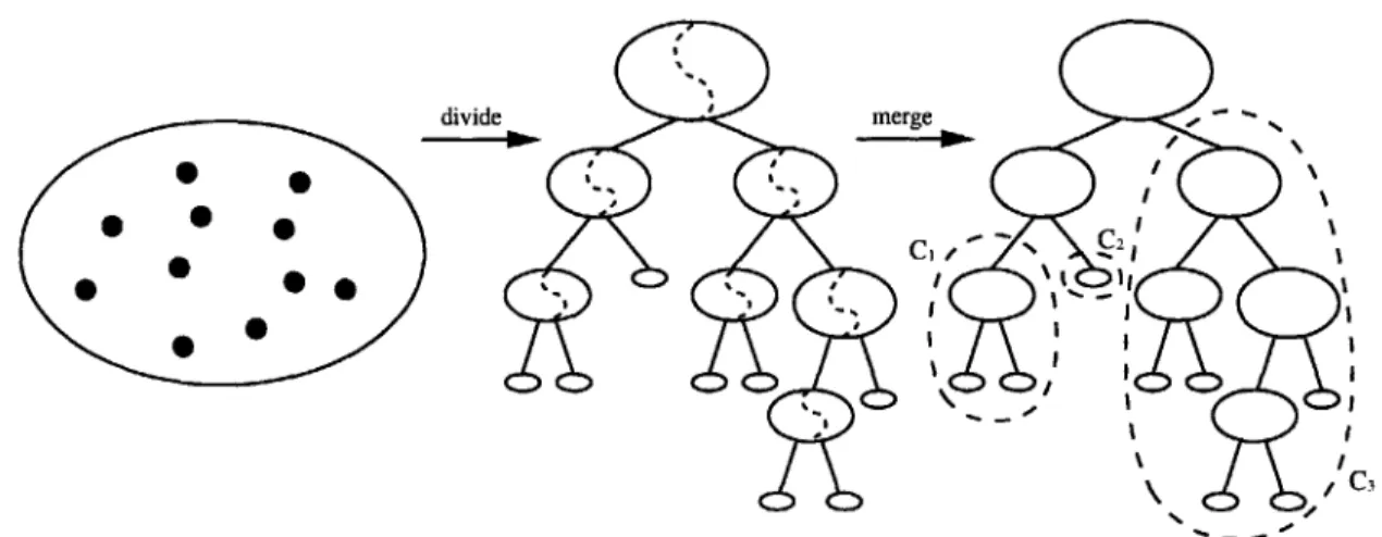
We present a divide-and-merge methodology for clustering. Our methodology combines the top-down and bottom-up approaches to hierarchical clustering. The methodology consists of two phases - the divide phase and the merge phase. In the divide phase, a top-down algorithm is used to recursively partition a set of objects into two pieces, forming a hierarchical clustering tree where the root is the set of all objects, and the leafs are the objects themselves. In the merge phase, we start with each leaf as its own cluster and merge clusters going up the tree. For many natural clustering objective functions, the merge phase can be executed optimally, producing the best tree-respecting clustering.
For the divide phase, we suggest the spectral clustering algorithm from [KVV04] as an effective top-down algorithm. This algorithm produces a tree that has guarantees on its quality with respect to a natural objective function. We show how to implement the spectral clustering algorithm so that it is particularly efficient for sparse object-feature matrices, a common case in data mining. In this scenario, the objects are encoded as feature vectors and the similarity between two objects is their inner product. For an object-feature matrix with M nonzeros, our implementation computes a cut in
O(M log n) time; if each cut is balanced, the overall running time to construct a tree
is O(Mlog2n).
The merge phase takes as input the tree produced by the divide phase. We show how to use dynamic programming to compute the optimal tree-respecting clustering for many natural clustering objective functions such as k-means, k-min cut, and correlation clustering. By tree-respecting clustering, we mean any clustering that is defined by a subset of the nodes of the tree. For objective functions with parameters such as k, the number of clusters desired, the dynamic program computes the optimal j-clustering for all
j
<
k. Indeed, the merge phase can compute the Pareto curves of such objectivefunctions.
We perform an extensive experimental evaluation on real data sets such as text, microarray, and categorical data. In these experiments, the true clustering is known. For instance, in text data, the true clustering is a partition into documents which share the same topic. Our experiments show that a "good" clustering exists in the tree produced by the spectral algorithm. By a "good" clustering, we mean a clustering that agrees with the true clustering. Furthermore, we show that the merge phase can find this good clustering in the tree. Our results compare favorably with known results.
We also implement our algorithm in a meta-web search engine which clusters results from web searches. Lastly, we describe the use of the spectral clustering algorithm in a real-world prediction task: forecasting health care costs for patients, given medical claims data from previous years. Our results show that for the most costly patients, our method predicts better than classification trees, a popular data mining tool.
1.4
Organization of this thesis
We describe notation and preliminaries in Chapter 2 which covers the necessary tech-nical material for this thesis. In Chapter 3, we describe our results on low-rank matrix approximation. Chapter 4 covers our application of low-rank matrix approximation to projective clustering. Finally, Chapter 5 describes the divide-and-merge methodology and gives the results of our experimental evaluation.
1.5
Bibliographic Notes
Section 3.2 and Chapter 4 is joint work with Amit Deshpande, Luis Rademacher, and Santosh Vempala and appeared in the 2006 Symposium on Discrete Algorithms conference proceedings. Section 3.3 is joint work with Santosh Vempala and appeared in the Workshop on Clustering High Dimensional Data and its Applications, held at the 2005 SIAM International Conference on Data Mining. Most of Chapter 5 is joint work with David Cheng, Ravi Kannan, and Santosh Vempala and appeared in the 2005 Principles of Database Systems conference proceedings. The work in Chapter 5 on predicting health care costs is joint with Dimitris Bertsimas, Margret Bjarnad6ttir, and Santosh Vempala and is unpublished.
Chapter 2
Preliminaries and Notation
In this chapter, we describe the technical background for this thesis. The content of this chapter consists of notation we use throughout the thesis and standard results from linear algebra (see
[GL96]
for instance). The bulk of this material is used in Chapters 3 and 4.2.1
Probability, random variables, and expectation
For an event A, we write Pr (A) to denote the probability that event A occurs. Likewise, for a random variable X, we denote by E (X) the expectation of X. The random variable X may be vector-valued. In this case, E (X) is the vector having as components the expected values of the components of v.
We make use of Markov's inequality, which is a basic tail inequality for nonnegative random variables:
Theorem 1 (Markov's inequality). Let X > 0 be a random variable. Then: 1
Pr (X > kE (X)) <1 -. k
2.2
Linear algebra
For a matrix A E R"X, we denote by A( its ith row. We denote by
I|AIH1
the squared Frobenius norm. That is:m n
IJAI|2
= 1 1 A .i=1 j=1
For a subspace V C R" and a vector u E R", let 7rv(u) be the projection of u onto
v. If {vi,. .. ,Vk} is a basis for V, then
k
7rv(u) =
Z(vi
-u)vi.For a matrix A E R"X, we write 7rv(A) to denote the matrix whose rows are the projection of the rows of A onto V. For a subset S of the rows of A, let span(S) 9 R" be the subspace generated by those rows; we use the simplified notation irs(A) for
lrspan(S)(A)-For subspaces V, W C R", the sum of these subspaces is denoted by V + W and is given by:
V +W= {v +w E Rn : v E Vw E W}.
We denote by V' the orthogonal subspace to V, i.e.
V' = {u E R : -v(u) = 0}.
We use the following elementary properties of the operator 7rv:
Proposition 2. For any A E R and matrices A, B E Rrnxn:
irv(AA + B) = Xiv(A) + irv(B).
Proposition 3. Let V, W C Rn be orthogonal subspaces. For any matrix A E Rmxn,
7rv+w(A) = nv(A) + 7rw(A).
2.2.1 Singular Value Decomposition
The singular value decomposition (SVD) of a matrix A E Rmx" is one of the most useful matrix decompositions. The property of the SVD we use in this thesis is that it gives the best rank k approximation to A for all k simultaneously. We first give a definition and then prove that every matrix A admits such a decomposition.
Definition 4. The singular value decomposition of a matrix A E Rxn is the
decom-position:
A = U:VT
where U E R"", E E Rmxn, and V E RfXf. The columns of U form an orthonormal
basis {u(), ... , u()} for R" and are called the left singular vectors of A. The columns
of V form an orthonormal basis {v(1), ... ,v)
}
for RI and are called the right singularvectors of A. E is a diagonal matrix, and the entries on its diagonal a, ... Ur are defined
as the singular values of A, where r is the rank of A. The left and right singular vectors
have the following property: Av() = uu(') and ATu(i) = -V(i).
Theorem 5. Any matrix A E R"xn admits a singular value decomposition.
Proof. We rely on the Spectral Theorem from linear algebra: every real, symmetric
matrix M G R"X" has n, mutually orthogonal eigenvectors
[Art91].
To prove that every matrix A E Rmxn admits a singular value decomposition, we apply the Spectral theorem to the following two matrices: AAT E R"nxr" and
ATA E R""". It is easy to see that these two matrices are symmetric. Let U, V be
the matrices whose columns are the eigenvectors promised by the Spectral Theorem for AAT and ATA.
Consider 0). Since it is an eigenvector of ATA, we have that:
AT Av(i) = v(.
Multiplying on the left by A, we get:
AAT( Av(i)) = A Av()
i.e. Av() points in the same direction as some eigenvector 0) of AAT. Therefore,
Av(i)/\|Av()J = U(0). Note that
itAv()I||
2 = (Av(i))T(Av(i))= v(i)AT Av( ) = A. So
we let ci = V5 - this implies that Av( = oau). Proving that ATu(i) = -(i) is
similar. This gives us the promised behavior of U and V. Finally, it is easy to check
that A = UEVT.
Define Ak E Rmx to be the matrix of rank k minimizing ||A - Ak I| for all matrices of rank k. The SVD of A gives Ak for every k - Ak = UE>kVT, where Ek is the matrix
E with its last r - k values on its diagonal zeroed out. Let Uk and Vk be the matrices
containing the first k columns of U and V, respectively. Note that Ak = AVkVT =
irly(A), since AVk = UkEk by the relationship between the left and right singular
vectors. For this reason, we often refer to Ak as the spectral projection of A, since it is the projection of A onto the top k right singular vectors of A. We prove that
Ak = 7rv,(A), i.e. the subspace Vk is the best rank-k subspace to project to, in the sense that it minimizes I|A - irw(A) 112 for any subspace W of rank k.
Theorem 6. Let A E Rmxn, and let k < n. Let Vk be the subspace spanned by the top
k right singular vectors of A. Then we have that:
||A -1yrvk(A)I 2= min ||A -,rw(A)II1
W:rank(W)=k
Proof. Note that, for any subspace W,
IAI|2
= IA - 7rw(A)||1 + ||2w(A)||1since the rows of A - irw(A) are orthogonal to the rows of irw(A). Thus, if IA -wry,(A)| 12is minimal, then I7rvk(A)I|1 is maximal; this is what we will prove.
Let W be an arbitrary subspace of dimension k spanned by the orthogonal vectors
WI,..., Wk. Recall that the columns of Vk are denoted by v(,.. ., v(k) and that these
columns are orthogonal. By the fact that w1i,... , Wk is a basis, we have that:
k
1\1 rw (A)|112 = ( ||Awms|2
i=1
For each wi, project w onto v('),..., v(), the n right singular vectors of A that span R":
n
Wi = Zaiv(i)
where aij = (w, - V u).
Since Av) ... Av(') is an orthogonal set of vectors, we have that for every i:
n1 n
I|Awil|
2 = Z JIAv )l|2 = a 2j=1 j=1
So for the projection of the entire matrix A, we have:
k n
W7rw(A)112F = .
i=1 j=1
Consider the "weight" 1 = _>v())2 (j(w.. on each a?. This weight is at most the norm of the projection of 0) on the subspace W, so it is bounded by 1, i.e.
k
Z(wi - v())2 < |I7rw(vj)||2 1
i=1
Furthermore, the sum of all the weights
Z" ZFU=
= E,_(w - v=W)2 isexactly k, since it is the norm of the projection of the vectors w1,..., Wk onto Vk:
k n k
ZZEwi - V v(wi)|2 k = k.
i=1 j=1 i=1
It follows that the maximum value that |7rw(A)| 2 can obtain is i=u o. Since Vk achieves this value, we have the desired result. 0
We will also use the fact that Ak is the best rank-k approximation with respect to the 2-norm as well.
Theorem 7.
Chapter 3
Low Rank Matrix Approximation
3.1
Introduction
In this chapter, we describe our results on low-rank matrix approximation. Let A E
Rmn be a matrix. The low-rank matrix approximation of A is a matrix B of rank k
such that
||A - BI|1
is minimized over all rank k matrices. Geometrically, the problem amounts to finding the best-fit subspace for the points in A. Consider the rows of A and Ak to be points in R". Then Ak are the points lying in a k-dimensional subspace that best fits the points of A. We refer interchangeably to Ak as the low-rank approximation of A and the spectral projection of A (see Chapter 2). In Figure 3-1, we show a depiction of low-rank matrix approximation for n = 3 and k = 2, i.e. finding a best-fit plane for points in 3 dimensions.
In our example, the points are the rows of the matrix A. The span of the points of Ak is the plane, which is the best-fit plane because it minimizes the sum of squared distances between points in A and their projections to the plane.
3.1.1 Motivation
Low-rank matrix approximation has seen many uses in data mining and analysis. By projecting data to a lower dimension, not only is the size of the data reduced, but the structure of the data is also often highlighted. This ability of low-rank matrix approx-imation to highlight underlying structure has been used in systems for collaborative filtering and information retrieval.
The classical methods for computing low rank matrix approximation work by com-puting the Singular Value Decomposition of A (see Chapter 2); they form the matrices
U, E, and V such that:
A = UEVT.
Recall that the matrix formed by zeroing out the last n - k singular values on the
0 -0 --0
Figure 3-1: The best-fit plane for points in 3 dimensions
O(min{mn2, nm2}) time, which may be too large for some applications. These
al-gorithms also assume that the entire matrix fits in main memory. However, some data sets may be too large to store/process in their entirety. For these data sets, a more appropriate model is the streaming model of computation, where one only has sequential access to the data and is allowed a few passes. The problem of finding approximations to the matrix B very quickly has received much attention in the past decade [FKV04, DKF+04, AM01, DK03, DKM06]. In Section 3.2 of this chapter, we give a new algorithm for low-rank matrix approximation and show small certificates for better additive approximation as well as relative approximation. At the heart of our work is a new distribution from which to sample the matrix A.
An area in which low-rank matrix approximation has seen much use is document clustering. In this problem, an algorithm is given a document set where documents naturally partition according to topic. The desired output of the algorithm is the natural partition according to topic. Many algorithms that use the low-rank matrix approximation of the document-term matrix of the document set have been proposed and have shown impressive experimental results
[Bol98,
ZDG+01, DHZ+01, Dhi0l, ZK02, XLG03, LMOO4]. These algorithms have been able to classify documents ac-cording to their topic much more effectively than traditional clustering algorithms such as k-means. However, their use of low-rank matrix approximation is varied -some methods only use one singular vector, while others use k, etc. Their varied use along with their common experimental success has motivated the question: do the algorithms share a common benefit from using spectral methods? Both theoret-ical and experimental work has been done to explain the success of these methods [PRTVOO, AFK+01, KVV04, McSO1, VWO4, KSV05, DM01, SS97]. The theoretical work has largely focused on proposing models for document sets and proving that spe-cific spectral algorithms succeed in these models, while the practical work has studied slightly different dimension-reduction techniques or the benefit of low-rank matrix ap-proximation for a specific algorithm. In Section 3.3, we propose the common benefitthat these methods share is based on two simple properties: approximation and dis-tinguishability. Both of these properties are independent of specific spectral clustering algorithms.
3.1.2
Our work
We first describe our work on improved approximation for low-rank matrix approxi-mation and then describe results on the benefit of spectral projection for document clustering. The results on improved approximation appear in Section 3.2 and the re-sults on the benefit of spectral projection appear in Section 3.3.
Improved approximation for low-rank matrix approximation
Frieze et al. [FKV04] showed that any matrix A has a subset of k/e rows whose span contains an approximately optimal rank-k approximation to A. In fact, the subset of rows can be obtained as independent samples from a distribution that depends only on the lengths of the rows. The approximation is additive.
Theorem 8 ([FKV04]). Let S be a sample of s rows of an m x n matrix A, where
each row is chosen independently from the following distribution:
Pr (A(') is picked) ; c I JAW 11
2
If s > k/ce, then the span of S contains a matrix Ak of rank at most k for which
E(IIA
- 11 |) < ||A - Ak 12+ E|Al\1.This theorem can be turned into an efficient algorithm based on sampling [DKF+04]
'. The algorithm makes one pass through A to figure out the sampling distribution and
another pass to sample and compute the approximation. It has additive error
chIA\IF
and its complexity is O(min{m, n}k2/E4).
In Section 3.2, we generalize Theorem 8. We show how to sample in multiple rounds and reduce the additive error exponentially in the number of rounds. We also describe how to combine volume sampling [DRVW06] with adaptive sampling to obtain
a relative approximation.
The generalization of Theorem 8 is that we can sample in multiple rounds, rather than just once. To take full advantage of sampling in multiple rounds, we must adapt our distribution based on samples from previous rounds. Suppose we have already
sampled a set of rows. Instead of picking rows with probability proportional to their length again, we pick rows with probability proportional to their length orthogonal to the subspace V spanned by our current samples. We prove an analog to Theorem 8,
but show that the additive error is proportional to hirv(A)IJ instead of IIA11'. This
'Frieze et al. go further to show that there is an s x s submatrix for s = poly(k/E) from which the
theorem gives rise to a multi-pass algorithm that proceeds in t rounds over. the matrix. The algorithm has additive error ci1AIIj, i.e. the additive error drops exponentially in the number of rounds. These results can be found in Section 3.2.2.
In Section 3.2.3, we show how to combine volume sampling [DRVW06] with adaptive sampling to obtain a relative approximation. Volume sampling is a generalization of [FKV04] where subsets of rows, rather than individual rows, are sampled. The result on relative approximation states that every matrix A contains a subset of k+k(k+ 1)/E rows in whose span lies a matrix Ak such that:
|A - k|12 < (1 + E)I|A -
AkI1-Benefit of Spectral Projection for Document Clustering
Document clustering is a fundamental problem in information retrieval; it has been used to organize results of a query [CKPT92] and produce summaries of documents [HKH+01]. Varied spectral methods for document clustering have been proposed which give impressive experimental results [Bol98, SS97, ZDG+01, DHZ+01, Dhi0l, ZK02, XLG03, LMOO4, CKVW05]. In Section 3.3, we attempt to explain the experimental success of these methods. We focus on spectral projection and give experimental evi-dence that clustering algorithms that use the spectral projection of a document-term matrix do indeed share a common benefit in the form of two properties: approximation and distinguishability. The second property explains why traditional clustering algo-rithms such as k-means perform better on the spectral projection of a document-term matrix than on the document-term matrix itself.
The first property, approximation, means that the spectral projection of a document-term matrix remains close to the original document-document-term matrix. Thus, spectral projec-tion reduces the dimension of the data, which speeds up clustering algorithms running on the data, while not incurring too much error. The experiments and results are described in Section 3.3.2.
The second property, distinguishability, is that clusters are more clearly demarcated after spectral projection. In particular, for natural (and commonly used) definitions of distance and similarity for documents, we give experimental evidence that inter-cluster distance/similarity is substantially more distinguishable from intra-inter-cluster dis-tance/similarity after spectral projection. Before spectral projection, these two quanti-ties are indistinguishable. This explains why clustering algorithms that work solely on the basis of pairwise distances/similarities perform better on the projection compared to the original document-term matrix. This property of spectral projection coincides with recent theoretical work on spectral algorithms for learning mixtures of distribu-tions [VWO4, KSV05]. We explain this connection and the experimental results in Section 3.3.3.
3.2
Improved Approximation for Low-Rank Matrix
Approximation
In this section, we describe our results on improved approximation for low-rank matrix approximation.
3.2.1
Related work
The work of Frieze et al. [FKV04] and Drineas et al. [DKF+04] introduced matrix sampling for fast low-rank approximation. Subsequently, an alternative sampling-based algorithm was given by Achlioptas and McSherry[AM01). That algorithm achieves slightly different bounds (see [AM01] for a detailed comparison) using only one pass. It does not seem amenable to the multipass improvements presented here. Bar-Yossef [BY03] has shown that the bounds of these algorithms for one or two passes are optimal up to polynomial factors in 1/c.
These algorithms can also be viewed in the streaming model of computation [MH98]. In this model, we do not have random access to data. Instead, the data comes as a stream and we are allowed one or a few sequential passes over the data. Algorithms for the streaming model have been designed for computing frequency moments [NA99], histograms [GKS06], etc. and have mainly focused on what can be done in one pass. There has been some recent work on what can be done in multiple passes [DK03, FKM+05]. The "pass-efficient" model of computation was introduced in [MH98]. Our multipass algorithms fit this model and relate the quality of approximation to the number of passes. Feigenbaum, et. al [FKM+05] show such a relationship for computing the maximum unweighted matching in bipartite graphs.
The Lanczos method is an iterative algorithm that is used in practice to compute the Singular Value Decomposition [GL96, KM04]. An exponential decrease in an additive error term has also been proven for the Lanczos method under a different notion of additive error ([GL96, KM04]). However, the exponential decrease in error depends on the gap between singular values. In particular, the following is known for the Lanczos method: after k iterations, each approximate singular value 0, obeys:
o2 > o - CkC
where both c and C depend on the gap between singular values. This guarantee can be transformed into an inequality:
||A -Ak1 ! <_A - AkJI -+ cC
very similar to the one we prove, but without the multiplicative error term for IIA
-Ak 12. In the Lanczos method, each iteration can be implemented in one pass over
A, whereas our algorithm requires two passes over A in each iteration. Kuczynski and Wozniakowski [KW92] prove that the Lanczos iteration, with a randomly chosen starting vector v, achieves a multiplicative error with respect to o in log(n)/v it-erations. However, this multiplicative error is not equivalent to a multiplicative error with respect to IA - A1 12}.
4 S S 0 S 0 0
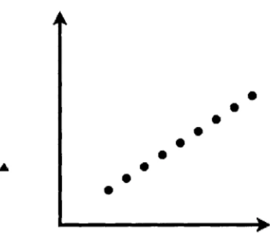
Figure 3-2: Only the circle points will be selected in the first round
3.2.2 Adaptive sampling
We motivate adaptive sampling with the following example. Consider Figure 3-2, and note that the circle points all lie along a single line. Therefore, the best rank-2 subspace has zero error. However, one round of sampling will most likely miss the triangle point and thus incur an error. So we use a two-round approach. In the first pass, we get a sample from the squared length distribution. We will likely only have circle points in this sample. Then we sample again, but adaptively, i.e. with probability proportional to the squared distance to the span of the first sample. Adaptive sampling ensures that with high probability we obtain the triangle point. The span of the full sample now contains a good rank 2 approximation.
The next theorem is very similar to Theorem 8 [FKV04]. However, instead of sampling rows according to their squared lengths, we sample rows according to their squared lengths orthogonal to a subspace V. Instead of obtaining a result with additive error proportional to |IA|II , we obtain additive error proportional to I|7rv (A)J1', the sum of the squared lengths of the rows of A orthogonal to V.
Theorem 9. Let A E R"'x be a matrix, V C R' be a subspace, and E = lrv: (A). Let S be a sample of s rows of an m x n matrix A, each chosen independently from the
following distribution:
Pr (A(') is picked) = ||E|
112
Then, for any nonnegative integer k, V +span(S) contains a matrix Ak of rank at most
k such that:
Es(I|A - Ak11) ; |A - Ak112 + -1|E 11.
and show that W is a good approximation to span{v('),... ,v(k)} in the sense that:
Es(JJA - rw(A)j|1)
1
|A - Ak||1 + -IIEI||.F F 8 s (3.1)
Recall that Ak = irspan{v(1),...,V(k)}(A), i.e. span{v(1),. . ., v(k)} is the optimal subspace
upon which to project. Proving (3.1) proves the theorem, since W C V + span(S). Let P = Pr (A(') is picked) = 112 . Define X(4 to be a random variable such that
U)
XU) i E()=
(A)
Ui(A(') - 7rv(A(')))
with probability P. Note that X/) is a linear function of a row of A sampled from the distribution D. Let X(A = E 1 X j, and note that Es(X()) = ETu().
For 1 < j k, define:
w) = rv(A)Tu(j) + X
Then we have that Es(wMi)) = ajvi). We seek to bound the error of w( with respect
to ajv(), i.e., Es(||w(i) - u3v()I112). We have that w( - o vW) = X(A - ETu(i), which
gives us
Es(llwdi) - O'jVW112) = Es((jX(j) - ETu(j)112)
= Es(IIXM||I12) - 2Es(XEi)) -ETu(i)
+
IIETu(
2= Es(IX(112) -
1ETu(i)11
2. (3.2)We evaluate the first term in (3.2),
= Es(IZ XW 11 2) l=1 2 AZEs( =1 - IiEEs( 1=1 ||X(i1|2) + 1S
2
2E
1<1 <12<S Es(X/j - Xj)IIX IU12) +S- 1 IIETu3) 11 2.
In (3.3) we used that X and X are independent. that
1
Z
Es(IIX 1(j)I2)(3.3)
From (3.2) and (3.3) we have
- IIETuA 1 2
The definition of Pi gives us:
Es(||Xi 112)| i=p 2
Es(llwed)
- jV() 112) =< IIE||1.