Towards quality assurance of software product lines with adversarial configurations

RESEARCH OUTPUTS / RÉSULTATS DE RECHERCHE

Author(s) - Auteur(s) :

Publication date - Date de publication :

Permanent link - Permalien :

Rights / License - Licence de droit d’auteur :

Bibliothèque Universitaire Moretus Plantin

Institutional Repository - Research Portal

Dépôt Institutionnel - Portail de la Recherche

researchportal.unamur.be

University of Namur

Towards quality assurance of software product lines with adversarial configurations

Temple, Paul; Acher, Mathieu; Perrouin, Gilles; Biggio, Battista; Jézéquel, Jean Marc; Roli,

Fabio

Published in:

SPLC 2019 - 23rd International Systems and Software Product Line Conference

DOI:

10.1145/3336294.3336309

Publication date:

2019

Document Version

Peer reviewed version

Link to publication

Citation for pulished version (HARVARD):

Temple, P, Acher, M, Perrouin, G, Biggio, B, Jézéquel, JM & Roli, F 2019, Towards quality assurance of

software product lines with adversarial configurations. in T Berger, P Collet, L Duchien, T Fogdal, P Heymans, T

Kehrer, J Martinez, R Mazo, L Montalvillo, C Salinesi, X Ternava, T Thum & T Ziadi (eds), SPLC 2019 - 23rd

International Systems and Software Product Line Conference. ACM International Conference Proceeding

Series, vol. A, ACM Press, 23rd International Systems and Software Product Line Conference, SPLC 2019,

co-located with the 13th European Conference on Software Architecture, ECSA 2019, Paris, France, 9/09/19.

https://doi.org/10.1145/3336294.3336309

General rights

Copyright and moral rights for the publications made accessible in the public portal are retained by the authors and/or other copyright owners and it is a condition of accessing publications that users recognise and abide by the legal requirements associated with these rights. • Users may download and print one copy of any publication from the public portal for the purpose of private study or research. • You may not further distribute the material or use it for any profit-making activity or commercial gain

• You may freely distribute the URL identifying the publication in the public portal ? Take down policy

If you believe that this document breaches copyright please contact us providing details, and we will remove access to the work immediately and investigate your claim.

Towards Quality Assurance of Software Product Lines with

Adversarial Configurations

∗

Paul Temple

NaDI, PReCISE, Faculty of Computer Science, University of Namur

Namur, Belgium

Mathieu Acher

Univ Rennes, IRISA, Inria, CNRS Rennes, France

Gilles Perrouin

NaDI, PReCISE, Faculty of Computer Science, University of Namur

Namur, Belgium

Battista Biggio

University of Cagliari Cagliari, Italy

Jean-Marc Jézéquel

Univ Rennes, IRISA, Inria, CNRS Rennes, France

Fabio Roli

University of Cagliari Cagliari, Italy

ABSTRACT

Software product line (SPL) engineers put a lot of effort to ensure that, through the setting of a large number of possible configuration options, products are acceptable and well-tailored to customers’ needs. Unfortunately, options and their mutual interactions create a huge configuration space which is intractable to exhaustively explore. Instead of testing all products, machine learning is increas-ingly employed to approximate the set of acceptable products out of a small training sample of configurations. Machine learning (ML) techniques can refine a software product line through learned con-straints and a priori prevent non-acceptable products to be derived. In this paper, we use adversarial ML techniques to generate adver-sarial configurations fooling ML classifiers and pinpoint incorrect classifications of products (videos) derived from an industrial video generator. Our attacks yield (up to) a 100% misclassification rate and a drop in accuracy of 5%. We discuss the implications these results have on SPL quality assurance.

CCS CONCEPTS

• Software and its engineering → Software product lines.

KEYWORDS

software product line; software variability; software testing; ma-chine learning; quality assurance

1

INTRODUCTION

Testers don’t like to break things; they like to dispel the illusion that things work. [33]

Software Product Line Engineering (SPLE) aims at delivering massively customized products within shortened development cy-cles [18, 47]. To achieve this goal, SPLE systematically reuses soft-ware assets realizing the functionality of one or more features, which we loosely define as units of variability. Users can specify products matching their needs by selecting/deselecting the features and provide additional values for their attributes. Based on such configurations, the corresponding products can be obtained as a result of the product derivation phase. A long-standing issue for developers and product managers is to gain confidence that all possible products are functionally viable, e.g., all products compile

∗_{Gilles Perrouin is an FNRS Research Associate. This research was partly supported}

by EOS Verilearn project grant no. O05518F-RG03. This research was also funded by the ANR-17-CE25-0010-01 VaryVary project.

and run. This is a hard problem, since modern software product lines (SPLs) can involve thousands of features and practitioners cannot test all possible configurations and corresponding products due to combinatorial explosion. Research efforts rely on variability models (e.g., feature diagrams) and solvers (SAT, CSP, SMT) to com-pactly define how features can and cannot be combined [2, 4, 5, 49]. Together with advances in model-checking, software testing and program analysis techniques, it is conceivable to assess the func-tional validity of configurations and their associated combination of assets within a product of the SPL [12, 13, 17, 39, 54, 57]. Yet, when dealing with qualities on the derived products (perfor-mance, costs, etc.), several unanswered challenges remain from the specification of feature-aware quantities to the best trade-offs be-tween products and family-based analyses (e.g., [36, 59]). In our industrial case-study, the MOTIV video generator [26], one can approximately generate 10314video variants. Furthermore, it takes about 30 minutes to create a new video: a non-acceptable (e.g., a too noisy or dark) video can lead to a tremendous waste of re-sources. A promising approach is to sample a number of config-urations and predict the quantitative or qualitative properties of the remaining configurations using Machine Learning (ML) tech-niques [29, 42, 48, 51, 52, 56, 58]. These techtech-niques create a pre-dictive model (a classifier) from such sampled configurations and infer the properties of yet unseen configurations with respect to their distribution’s similarity. This way, unseen configurations that do not match specific properties can be automatically discarded and constraints can be added to the feature diagram in order to avoid them permanently [55, 56]. However, we need to trust the ML classifier [1, 41] to avoid costly misclassifications. In the ML community, it has been demonstrated that some forged instances, called adversarial, can fool a given classifier [11]. Adversarial ma-chine learning (advML) thus refers to techniques designed to fool (e.g., [6, 7, 41]), evaluate the security (e.g., [9]) and even improve the quality of learned classifiers [27]. Our overall goal is to study how advML techniques can be used to assess quality assurance of ML classifiers employed in SPL activities. In this paper, we design a generator of adversarial configurations for SPLs and measure how the prediction ability of the classifier is affected by such adversarial configurations. We also provide scenarios of usage of advML for quality assurance of SPLs. We discuss how adversarial configura-tions raise quesconfigura-tions about the quality of the variability model or the testing oracle of SPL’s products. This paper makes the following contributions:

(1) An adversarial attack generator, based on evasions attacks and dedicated to SPLs;

(2) An assessment of its effectiveness and a comparison against a random strategy, showing that up to 100% of the attacks are valid with respect to the variability model and successful in fooling the prediction of acceptable/non-acceptable videos, leading to a 5% accuracy loss;

(3) A qualitative discussion on the generated adversarial con-figurations w.r.t. to the classifier training set, its potential improvement and the practical impact of advML in the qual-ity assurance workflow of SPLs.

(4) The public availability of our implementation and empirical results at https://github.com/templep/SPLC_2019

The rest of this paper is organized as follows: Section 2 presents the case study and gives background information about ML and advML; Section 3 shows how advML is used in the context of MOTIV; Section 4 describes experimental procedures and discusses results; Section 5 and 6 present some potential threats that could mitigate our conclusions and propose qualitative discussions about how adversarial configurations could be leveraged for SPLs developers. Section 7 covers related work and Section 8 wraps up the paper with conclusions.

2

BACKGROUND

2.1

Motivating case: MOTIV generator

MOTIV is an industrial video generator which purpose is to provide synthetic videos that can be used to benchmark computer vision based systems. Video sequences are generated out of configurations specifying the content of the scenes to render [56]. MOTIV relies on a variability model that documents possible values of more than 100 configuration options, each of them affecting the perception of generated videos and the achievement of subsequent tasks, such as recognizing moving objects. Perception’s variability relates to changes in the background (e.g., being a forest or buildings), ob-jects passing in front of the camera (with varying distances to the camera and different trajectories), blur, etc. There are 20 Boolean options, 46 categorical (encoded as enumerations) options (e.g., to use predefined trajectories) and 42 real-value options (e.g., dealing with blur or noise). Precisely, in average, enumerations contain about 7 elements each and real-value options vary between 0 and 27.64 with a precision of 10−5. Excluding (very few) constraints in the variability model, we over-estimate the video variants’ space size: 220∗ 746∗ ((0 − 27.64) ∗ 105)42 ≈ 10314. Concretely, MOTIV takes as input a text file describing the scene to be captured by a synthetic camera as well as recording conditions. Then, Lua [32] scripts are called to compose the scene and apply desired visual effects resulting in a video sequence. To realize variability, the Lua code use parameters in functions to activate or deactivate options and to take into account values (enumerations or real values) de-fined into the configuration file. A highly challenging problem is to identify feature values and interactions that make the identification of moving objects extremely difficult if not impossible. Typically, some of the generated videos contain too much noise or blur. In other words, they are not acceptable as they cannot be used to bench-mark object tracking techniques. Another class of non-acceptable videos is composed of the ones in which pixels value do not change,

Variability model Sampling method Configuration files

Generating the training set

…

Derivation (Lua generator)

Oracle (Video Quality Assessment) … Labeling Machine learning J48 tree signal_quality.luminance_dev signal_quality.luminance_dev signal_quality.luminance_dev capture.local_light_change_level 0 (110.0/1.0) 0 (2.0) 1 (27.0) 1 (4.0) 0 (3.0) > 21.3521 <= 21.3521 <= 1.01561> 1.01561 <=18.1437>18.1437 <=0.401449 > 0.401449 Variability model + cst1 ^ cst2 ^ … Constraints Constraints extractor

Constraining the original variability model

Testing the training set

Separating model using machine learning

Figure 1: Refining the variability model of MOTIV video gen-erator via an ML classifier.

resulting in a succession of images for which all pixels have the same color: nothing can be perceived. As mentioned in Section 1, non-acceptable videos represent a waste of time and resources: 30 minutes of CPU-intensive computations per video, not including to run benchmarks related to object tracking (several minutes de-pending on the computer vision algorithm). We therefore need to constraint our variability model to avoid such cases.

2.2

Previous work: ML and MOTIV

We previously used ML classification techniques to predict the acceptability of unseen video variants [56]. We summarise this process in Figure 1.

We first sample valid configurations using a random strategy (see Temple et al. [56] for details) and generate the associated video sequences. A computer program playing the role of a testing or-acle labels videos as acceptable (in green) or non-acceptable (in red). This oracle implements image quality assessment [23] defined by the authors via an analysis of frequency distribution given by Fourier transformations. An ML classifier (in our case, a decision tree) can be trained on such labelled videos. “Paths" (traversals from the top to the leaves) leading to non-acceptable videos can easily be transformed into new constraints and injected in the variability model. An ML classifier can make errors, preventing acceptable videos (false negatives) or allowing non-acceptable videos (false positives). Most of these errors can be attributed to the confidence of the classifier coming from both its design (i.e., the set of ap-proximations used to build its decision model) and the training set (and more specifically the distribution of the classes). Areas of low confidence exist if configurations are very dissimilar to those already seen or at the frontier between two classes. We use advML to quantify these errors and their impact on MOTIV.

2.3

ML and advML

ML classification. Formally, a classification algorithm builds a func-tionf : X 7→ Y that associates a label in the set of predefined classes y ∈ Y with configurations represented in a feature space (noted x ∈ X ). In MOTIV, only two classes are defined: Y = {−1, +1}, respectively representing acceptable and non-acceptable videos.X represents a set of configurations and the configuration space is defined by configuration options of the underlying feature model (and their definition domain). The classifierf is trained on a data setD constituted of a set of pairs (x_it,y_it) wherext ∈X is a set of

Figure 2: Adversarial configurations (stars) are at the limit of the separating function learned by the ML classifier valid configurations from the variability model andyt ∈Y their associated labels. To label configurations inD, we use an oracle (see Figure 1). Once the classifier is trained,f induces a separation in the feature space (shown as the transition from the blue/left to the white/right area in Figure 2) that mimics the oracle: when an unseen configuration occurs, the classifier determines instantly in which class this configuration belongs to. Unfortunately, the separation can make prediction errors since the classifier is based on statistical assumptions and a (small) training sample. We can see in Figure 2 that the separation diverges from the solid black line representing the target oracle. As a result, two squares are misclassified as being triangles. Classification algorithms realise trade-offs between the necessity to classify the labelled data correctly, taking into account the fact that it can be noisy or biased and its ability to generalise to unseen data. Such trade-offs lead to approximations that can be leveraged by adversarial configurations (shown as stars in Figure 2). AdvML and evasion attacks. According to Biggio et al. [11], delib-erately attacking an ML classifier with crafted malicious inputs was proposed in 2004. Today, it is called adversarial machine learning and can be seen as a sub-discipline of machine learning. Depend-ing on the attackers’ access to various aspects of the ML system (dataset, ability to update the training set) and their goals, various kinds of attacks [6–10] are available: they are organised in a taxon-omy [1, 11]. In this paper, we focus on evasion attacks: these attacks move labelled data to the other side of the separation (putting it in the opposite class) via successive modifications of features’ values. Since areas close to the separation are of low confidence, such ad-versarial configurations can have a significant impact if added to the training set. To determine the direction to move the data towards the separation, a gradient-based method has been proposed by Big-gio et al. [6]. This method requires the attacked ML algorithm to be differentiable. One of such differentiable classifiers is the Support Vector Machine (SVM), parameterizable with a kernel function1.

3

EVASION ATTACKS FOR MOTIV

3.1

A dedicated Evasion Algorithm

Algorithm 1 presents our adaptation of Biggio et al.’s evasion attack [6]. First, we select an initial configuration to be moved (x0_{): selection trade-offs are discussed in the next section. Then,}

1_{most common functions are linear, radial based functions and polynomial}

Algorithm 1 Our algorithm conducting the gradient-descent eva-sion attack inspired by [6]

Input: x0_{, the initial configuration; t, the step size; nb_disp, the}

number of displacements; g, the discriminant function Output:x∗, the final attack point

(1) m = 0;

(2) Setx0to a copy of a configuration of the class from which the attack starts;

whilem < nb_disp do (3) m = m+1;

(4) Let ∇F (xm−1_{) a unit vector, normalisation of ∇д(x}m−1_);

(5)xm=xm−1−t∇F (xm−1); end while

(6) returnx∗=xm;

we need to set the step size (t), a parameter controlling the vergence of the algorithm. Large steps induce difficulties to con-verge, while small steps may trap the algorithm in a local optimum. While the original algorithm introduced a termination criterion based on the impact of the attack on the classifier between each move (if this impact was smaller than a thresholdϵ, the algorithm stopped; assuming an optimal attack) we fixed the maximal number of displacementsnb_disp in advance. This allows for a controllable computation budget, as we observed that for small step sizes the number of displacements required to meet the termination criterion was too large. The functionд is the discriminant function and is defined by the ML algorithm that is used. It is defined asд : X 7→ R that maps a configuration to a real number. In fact, only the sign ofд is used to assign a label to a configuration x. Thus, f : X 7→ Y can be decomposed in two successive functions: firstд : X 7→ R that maps a configuration to a real value and thenh : R 7→ Y with h = siдn(д). However, |д(x)| (the absolute value of д) intuitively re-flects the confidence the classifier has in its assignment ofx. |д(x)| increases whenx is far from the separation and surrounded by other configurations from the same class and is smaller whenx is close to the separation. The term discriminant function has been used by Biggio et al. [6] and should not be confused with the unre-lated discriminator component of GANs by Goodfellow et al. [27]. In GANs, the discriminator is part of the “robustification process". It is an ML classifier striving to determine whether an input has been artificially produced by the other GANs’ component, called the generator. Its responses are then exploited by the generator to produce increasingly realistic inputs. In this work, we only gen-erate adversarial configurations, though GANs are envisioned as follow-up work.

Concretely, the core of the algorithm consists of thewhile loop that iterates over the number of displacements. Statement (4) de-termines the direction towards the area of maximum impact with respect to the classifier (explaining why only a unit vector is needed). ∇д(xm−1) is the gradient ofд(xm−1) and the direction of interest towards which the adversarial configuration should move. This vector is then multiplied by the step sizet and subtracted to the previous move (5). The final position is returned after the number of displacements has been reached. For statements (4) and (5) we simplified the initial algorithm [6]: we do not try to mimic as much

as possible existing configurations as we look forward to some diversity. In an open ended feature space, gradient can grow indef-initely possibly preventing the algorithm to terminate. Biggio et al. [6] set a maximal distance representing a boundary of the feasi-ble region to keep the exploration under control. In MOTIV, this boundary is represented by the hard constraints in the variability model. Because of the heterogeneity of MOTIV features, cross-tree constraints and domain values are difficult to specify and enforce in the attack algorithm. SAT/SMT solvers would slow down the attack process. We only take care of the type of feature values (natural integers, floats, Boolean). For example, we reset to zero natural integer values that could be negative due to displacements or we ensure that Boolean values are either 0 or 1.

As introduced in Section 2, decision trees are not directly com-patible with evasion attacks as the underlying mathematical model is highly non-linear making it non-derivable (forbidding to com-pute a gradient). We learn another classifier (i.e., a Support Vector Machine) on which we can perform evasion attacks directly [6, 11]. We rely upon evidence that attacks conducted on a specific ML model can be transferred to others [14, 20, 21].

3.2

Implementation

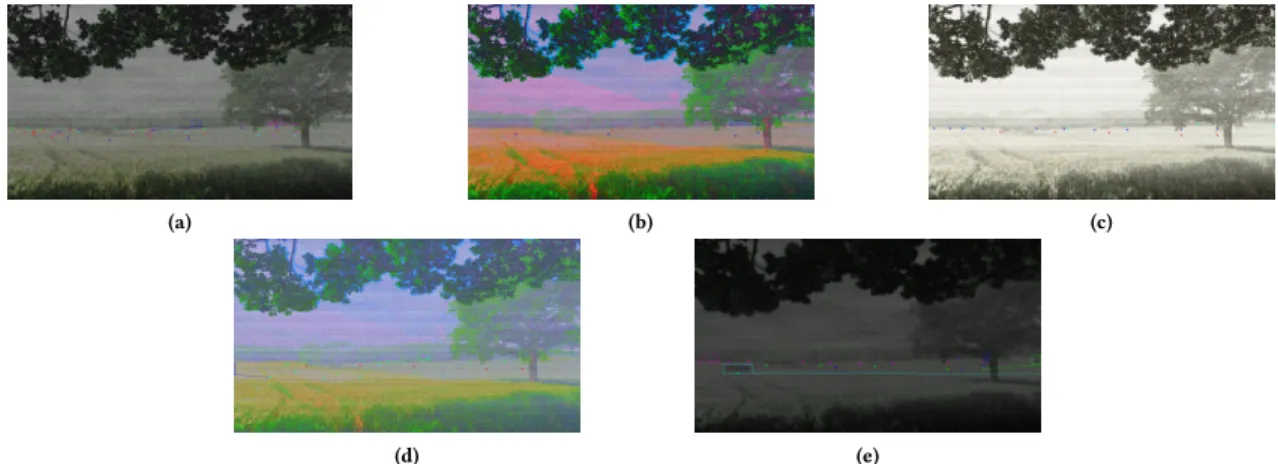
We implemented the above procedure in Python 3 (scripts available on the companion website). Figure 3 depicts some images of videos generated out of adversarial configurations.

MOTIV’s variability model embeds enumerations which are usu-ally encoded via integers. The main difference between the two is the logical order that is inherent to integers but not encoded into enumerations. As a result, some ML techniques have difficulties to deal with them. The solution is to “dummify" enumerations into a set of Boolean features, which truth values take into account exclusion constraints in the original enumerations. Conveniently, Python provides the get_dummies function from the pandas library which takes as input a set of configurations and feature indexes to dummify. For each feature index, the function creates and re-turns a set of Boolean features representing the literals’ indexes encountered while running through given configurations: if the get_dummies function detects values in the integer range [0, 9] for a feature associated to an enumeration, it will return a set of 10 Boolean features representing literals’ indexes in that range. It also takes care or preserving the semantics of enumerations. However, dummification is not without consequences for the ML classifier. First, it increases the number of dimensions: our 46 initial enu-merations would be transformed into 145 features. Doing so may expose the ML algorithm to the curse of dimensionality [3]: as the number of features increases in the feature space, configurations that look alike (i.e., with close feature values and the same label) tend to go away from each other, making the learning process more complex. This curse has also been recognised to have an impact on SPL activities [19]. Dummification implies that we will operate our attacks in a feature space essentially different from the one induced by the real SPL. This means that we need to transpose the generated attacks in the dummified feature space back to the original SPL one, raising one main issue: there is no guarantee that an attack relevant in the dummified space is still efficient in the reduced original space (the separation may simply not be the same).

Additionally, gradient methods operate per feature only, meaning that exclusion constraints in dummified enumerations are ignored. That is, when transposed back to the original configuration space, invalid configurations would need to be “fixed", potentially putting these adversarial configurations away from the optimum computed by the gradient method. For all these reasons, we decided to operate on the initial feature space, acknowledging the threat of considering enumerations as ordered. We conducted a preliminary analysis2 that showed that the order of the importance of the features were kept whether we use a dummified or the initial feature space. So this threat is minor in comparison of the pitfalls of dummification. We do not make any further distinctions between the two terms since we use them without making any transformations.

As mentioned in Section 3.1, we conducted attacks on a support vector machine with a linear kernel since it was faster according to a preliminary experiment. Scripts as well as data used to compare predictions can be found on the companion webpage.

4

EVALUATION

4.1

Research questions

We address the following research questions:

RQ1: How effective is our adversarial generator to synthesize ad-versarial configurations? Effectiveness is measured through the ca-pability of our evasion attack algorithm to generate configurations that are misclassified:

• RQ1.1: Can we generate adversarial configurations that are wrongly classified?

• RQ1.2: Are all generated adversarial configurations valid w.r.t. constraints in the VM?

• RQ1.3: Is using the evasion algorithm more effective than generating adversarial configurations with random modifi-cations?

• RQ1.4: Are attacks effective regardless of the targeted class? RQ2: What is the impact of adding adversarial configurations to the training set regarding the performance of the classifier? The intuition is that adding adversarial configurations to the training set could improve the performance of the classifier when evaluated on a test set.

4.2

Evaluation protocol

Our evaluation dataset is composed of 4, 500 randomly sampled and valid video configurations, that we used in previous work [56]. We selected 500 configurations to train the classifier keeping a sim-ilar representation of non-acceptable configurations (10%, i.e., ≈ 50 configurations) compared to the whole set. The remaining 4, 000 configurations are used as a test set and also have a similar repre-sentation regarding acceptable/non-acceptable configurations. This setting contrasts with a common practice of using a high percent-age (i.e., around 66%) of available examples to train the classifier. However, due to the low number of non-acceptable configurations, such a setting is impossible.k-fold cross-validation is another com-mon practice used when few data points are available for training (4, 500 configurations is an arguably low number with respect to the size of the variant space). Cross-validation is used to validate/select

2_{available on the companion webpage: https://github.com/templep/SPLC_2019} 4

(a) (b) (c)

(d) (e)

Figure 3: Examples of generated videos using evasion attack a classifier when several are created, for instance when trying to

fine-tuned hyper-parameters, which is not our case here. Further-more, separating our 4, 500 configurations into smaller sets is likely to create a lot of sets without any non-acceptable configurations. None of these practices seem to be adapted to our case.

The key point is that only about 10% of configurations are non-acceptable. This is a ratio that we cannot control exactly as it de-pends from the targeted non-functional property. In order to re-duce imbalance, several data augmentation techniques exist like SMOTE [16]. Usually, they create artificial configurations while maintaining the configurations’ distribution in the feature space. In our case, we compute the centroid between two configurations and use it as a new configuration. Thanks to the centroid method, we can bring perfect balance between the two classes (i.e., 50% of acceptable configurations and non-acceptable configurations). Technically, we compute how many configurations are needed to have perfectly balanced sets (i.e., training and test sets): We select randomly two configurations from the less represented class and compute the centroid between them, check that it is a never-seen-before configuration and adds it to the available configurations. The process is repeated until the number of configurations required is reached. Once a centroid is added to the set of available configu-rations, it is available as a configuration to create the next centroid. In the remainder, we present the results with both original and balanced data sets in order to assess whether the impact of class representation imbalance on adversarial attacks. We configured our evasion attack generator with the following settings: i) we set the number of attacks points to generate 4000 configurations for RQ1 and 25 configurations for RQ2 as explained hereafter; ii) considered step size (t) values are {10−6_{; 10}−4_{; 10}−2_{; 1; 10}2_{; 10}4_{; 10}6_{}; iii) the}

number of iterations is fixed to 20, 50 or 100. To mitigate random-ness, we repeat ten times the experiments. All results discussed in this paper can also be found on our companion webpage3.

4.3

Results

4.3.1 RQ1: How effective is our adversarial generator to syn-thesize adversarial configurations?

To answer this question, we assess the number of wrongly clas-sified adversarial configurations over 4, 000 generations (and about

3_{https://github.com/templep/SPLC_2019}

7, 000 configurations when the training set is balanced) and com-pare them to a random baseline: to the best of our knowledge, there is no comparable evasion attack.

RQ1.1: Can we generate adversarial configurations that are wrongly classified?

For each run, a newly created adversarial (i.e., afternb_disp is reached) configuration is added to the set of initial configurations that can be selected to start an evasion attack. We therefore give a chance to previous adversarial configurations to continue further their displacement towards the global optimum of the gradient.

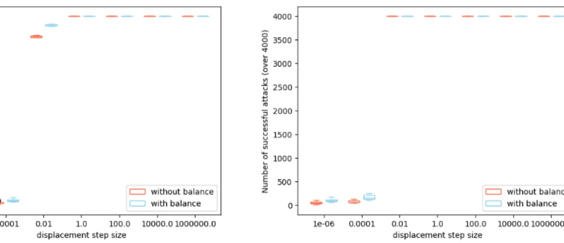
Figure 4 shows box-plots resulting of ten runs for each attack setting. We also show results when the training set is imbalanced (i.e., using the previous training set containing 500 configurations with about 10% of non-acceptable configurations) and when it is balanced (i.e., increasing the number of non-acceptable configu-rations using the data augmentation technique described above). Both Figure 4a and Figure 4b indicate that we can always achieve 100% of misclassified configurations with our attacks. Regarding Figure 4a, all generated configurations become misclassified when step size is set to 1.0 or a higher value. When 100 displacements are allowed (see Figure 4b), the limit appears earlier, i.e., whent equals 0.01. Similar results can be obtained when the number of maximum displacements is set to 50, the only difference is that witht set to 0.01 not all adversarial configurations are misclassified but about 3, 900 (97.5%) when the training set is imbalanced and about 3, 700 (92.5%) with a balanced set.

Discussion: Increasing the number of displacements require lower step sizes to reach the misclassification goal but it comes at the cost of more computations. However, increasing the number of displace-ments when the step size is already large results in incredibly large displacements, leading to invalid configurations in the MOTIV case. RQ1.2: Are all generated adversarial configurations valid w.r.t. constraints in the VM?

As discussed in Section 3, we perform a basic type check on fea-tures. However, this check does not cover specific constraints such as cross-tree ones. To ensure the full compliance of our adversarial configurations, we run the analysis realised by the MOTIV video generator. This includes, amongst others, checking the correctness features values with respect to their specified intervals.

Figure 5 shows on the X-axis the different step sizes while the Y-axis depicts the number of valid adversarial configurations w.r.t.

(a) Number of misclassified adversarial configurations (20 displace-ments)

(b) Number of misclassified adversarial configurations (100 displace-ments)

Figure 4: Number of successful attacks on class acceptable; X-axis represents different step size valuest while Y-axis is the number of misclassified adversarial configurations by the classifier. For eacht value, results with balanced and imbalanced training set are shown (respectively in blue and orange).

Figure 5: Number of valid attacks on class acceptable; X-axis represents different step sizet values; Y-X-axis reports the number of valid configurations. In red and blue are respec-tive results with an imbalance and a balance training set in terms of classes representation.

constraints. Regardless of the number of displacements and whether the training set is balanced, all results are the same except for Fig-ure 5 that presents one difference for a displacement step size of 100. One possible explanation is that when the training set is balanced, more configurations can be taken as a starting point of the evasion algorithm: the gradient descent procedure might lead the current attack towards a slightly different area in which configurations remain valid. Overall, regardless of the number of authorized dis-placements, we can see a clear drop of valid configurations from 4, 000 to 0 between step size set to 1 and 100.

Discussion: We can scope parameters such that adversarial config-urations are both successful and valid when step size is set between 0.01 and 1.0, regardless of the number of displacements. Increasing the step size leads to non-valid configurations while with smaller step sizes, adversarial configurations have not moved enough to cross the separation of the classifier (leading to unsuccessful at-tacks).

RQ1.3: Is using the evasion algorithm more effective than generating adversarial configurations with random displace-ments? Previous results of RQ1.1 and RQ1.2 show we are able to craft valid adversarial configurations that can be misclassified by the ML classifier, but is our algorithm better than a random base-line? The baseline algorithm consists in: i) for each feature, choosing randomly whether to modify it; ii) choosing randomly to follow the slope of the gradient or going against it (the role of ‘-’ of line 5 in Algorithm 1 that can be changed into a ‘+’); iii) choosing ran-domly a degree of displacement (corresponding to the slope of the gradient (∇F (xm−1_{)) of line 5 in Algorithm 1). Both the step size}

and the number of displacements are the same as in the previous experiments.

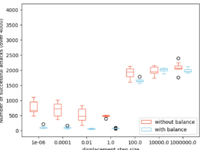
Figure 6 shows the ability of random attacks to successfully mislead the classifier. Random modifications are not able to exceed 2, 500 misclassifications (regardless of the number of displacements, the step size or whether the training set is balanced or not) which corresponds to more than half the generated configurations but with a lower effectiveness than with our evasion attack. The maximum number of misclassified configurations after random modifications starts from step sizet = 10, 000 regardless of the studied number of displacements.

Considering the validity of these configurations, results are sim-ilar to what can be observed in Figure 5. The only difference is that the transition from 4, 000 to 0 in the number of valid configurations is smoother and happens whent is in [0.01; 100].

(a) Number of successful random attacks after 20 displacements (b) Number of successful random attacks after 100 displacements

Figure 6: Number of successful random attacks on class acceptable; X-axis represents different step size valuest while Y-axis is the number of misclassified adversarial configurations by the classifier. In red and blue are respective results with an imbalance and a balance training set in terms of classes representation.

Discussion: Previous results show that the effectiveness of evasion attacks are superior to random modifications since i) evasion attacks are able to craft configurations that are always misclassified by the ML classifier while less than 2, 500 over 4, 000 generations will be misclassified using random modifications; ii) generated evasion attacks support a larger set of parameter values for which generated configurations are valid; iii) we were able to identify sweet spots for which evasion attacks were able to generate 4, 000 configurations that were both misclassified and valid.

RQ1.4: Are attacks effective regardless of the targeted class? Previously, we generated evasion attacks from the class non-acceptable and tried to make them acceptable for the ML classifier but is our attack symmetric? Now, we configure our adversarial configura-tion generator so that it moves configuraconfigura-tions from the class +1 (acceptable configurations) to the class -1 (non-acceptable).

Overall, the attack is symmetric: all generated adversarial con-figurations can be misclassified. Figure 7a shows that all generated configurations are misclassified when step size is set to 1 or higher with a number of displacements of 20 while, when the number of displacements is set to 100 (see Figure 7b), the step size can be set to 0.01 or higher. These observations are the same regardless of the balance in the training set.

Regarding the adversarial configuration validity, a transition from 4, 000 to 0 can still be observed. However, when the number of displacements is set to 20 or when the training set is balanced, the transition is abrupt and occurs when step size belongs to the range [100, 10, 000]. With a higher number of displacements (i.e., 50 and 100 and no balance), the transition is smoother but happens with smaller step sizes (i.e., witht in between [0.01; 100]. In the end, adversarial configurations can be generated regardless of the targeted class even if targeting the least represented class seems promising.

Our generated adversarial attacks are: 100% effective (al-ways misclassified, RQ1.1), do not depend on the target class (RQ1.4) and yield valid configurations (RQ1.2). In contrast, our random baseline was only able to achieve 62.5% of ef-fectiveness at best (RQ1.3). The balance in the training set does not affect these results and the targeted class affects show the same trends despite small differences (RQ1.4).

4.3.2 RQ2: What is the impact of adding adversarial con-figurations to the training set regarding the performance of the classifier? In our previous experiments, we only evaluated the impact of generated attacks in test sets. Yet, some ML techniques (GANs) take advantage of adversarial instances by incorporating them in the training set to improve the classifier confidence and possibly performance. In our context, we want to assess the impact of our attacks when our classifier includes them in the training dataset, especially with less “aggressive” (e.g., small step sizes and a low number of displacements) configurations of the attacks.

To do so, we allowed 20 displacements in order to avoid configu-rations moving too far from their initial positions and we restrict the step size to every power of 10 in between 10−4and 101. For each step size, we generate 25 adversarial configurations that are added all at once in the training set, we retrain the classifier and evaluate it on the configurations that constitute the initial test set (without any adversarial configurations in it). Every retraining pro-cess were repeated ten times in order to mitigate the effects of the random configuration selection and starting configurations. We also present results when the training set is balanced, in which case we have also augmented the test set to bring balance and to follow the same data distribution. In this case, the test set does not contain 4, 000 configurations but about 7, 000 in which 50% of the configurations are considered acceptable and the remaining are considered non-acceptable.

(a) Number of successful adversarial attacks after 20 displacements (b) Number of successful adversarial attacks after 100 displacements

Figure 7: Number of successful adversarial attacks on class non-acceptable; X-axis represents different step size valuest while Y-axis is the number of misclassified adversarial configurations by the classifier; In orange and blue are respectively shown results when the training set is not balanced and when it is.

Figure 8: Accuracy of the classifier after retraining with 25 adversarial configurations in the training set over a test set of 4, 000 configurations (7, 000 configurations when the train-ing set is balanced). In red are results when no balance are forced in the classes, in blue, both training set and test set are balanced. The initial accuracy of the classifier is represented by the horizontal line (96.4562% for the red line and 96.7143% for the blue one). X-axis represents different step size val-uest while Y-axis is the accuracy of the classifier (zoomed between 80% and 100%).

Figure 8 shows the accuracy of the retrained classifiers over a test set composed of 4, 000 configurations for the red part and 7, 000 configurations for the blue one.

The initial accuracy of the classifier was 96.4562% over the same 4, 000 configurations and is shown as the horizontal red line. We

make the following observations: i) using adversarial configura-tions in the training, even with low step sizes, tend to decrease the accuracy of the retrained classifier; ii) starting from step sizes of 1, every run gives the same result.

Specifically, with step size equals to 10−4, the median of the boxplot is very close to the initial accuracy (i.e., 96.4562%) of the classifier and the interquartile range is small suggesting that the impact of adding adversarial configurations into the training set is marginal. Between 10−3to 102, the median is slightly decreasing and the interquartile range tends to increase. Att = 10−1the accu-racy of the classifier drops to 91%, the adversarial configurations are specially efficient, forcing the ML classifier to change drastically its separation resulting in a lot of prediction errors. The last two step sizes shows that all the runs give the same results in terms of accuracy. Focusing on these runs, adversarial configurations had features with the same value: the amount of heat haze, of blur, of compression artefact or the amount of static noise of the 25 adver-sarial configurations are all equal. All of these features are directly related to the global quality of images, and are key for the classifier accuracy. We explain the evolution of the classifier’s accuracy as a combination of the contribution of the 8 most important features and the constraints of the VM. For low step sizes (t ∈ [10−4_{, 10}−2_]),

displacements are modest and therefore perturbations are very limited, though slightly observable. The sweet spot is att = 10−1: the resulting displacement is important enough to change feature values so that the associated configurations are moved effectively towards the separation and fool the classifier. We computed the means and standard deviations between the initial and adversarial configurations and their difference witnesses the impact of adver-sarial configurations on the classifier. For larger values oft (i.e., > to 10−1), these features lose their impact because their values are limited by constraints (so that they do not exceed the bounds).

In the case where training and test sets are balanced (in blue on Figure 8), results follow the same tendency. Since most of added

configurations to provide balance are well classified, we see that the accuracy is a bit higher than in the non-balanced case. Values remain close to the baseline, however, whent = 1.0, results are worse than for other executions as for the non-balanced setting. Yet, we cannot conclude about the classifier robustness and more experiments should be conducted to take into account the fact the balanced and non-balanced datasets do not contain the same number of configurations.

Our attacks cannot improve the classifier’s accuracy but can make it significantly worse: 25 adversarial configurations over 500 can make the accuracy drops by 5%. Successful attacks also pinpoint visual features that do influence the videos’ acceptability and that do make sense from the SPL perspective (computer vision).

5

THREATS TO VALIDITY

Internal threats. Choice of parameter values for our experiments may constitute a threat. The step size has been set to different pow-ers of 10, we only used 3 different number of allowed displacements (i.e., 20, 50 and 100). From our perspective, using step size of 10−7 in a highly dimensional space seems ridiculously small while, on the contrary, using step size of 104are tremendously large which motivates our choice to not going over these boundaries. However, the lower boundary could have been extended which might have affect results regarding RQ2. Still, given the design of our attack generator, it is likely that performance of the classifier would never have increased. Regarding the number of displacements, we could have used finer grained values. We sought a compromise between allowing a lot of small steps and a few big steps. Regarding the choice of evasion attacks, as presented in Section 2, several tech-niques exist. Evasion attacks showed interesting results and open new perspectives that we discuss in the Section 6.

We rely on centroids to deal with class imbalance (see Section 4.2). The centroid method has pros and cons: centroids are easy and quick to compute, new configurations tend to follow the same distribu-tion as they result in more densely populated clusters and on rare occasions, make clusters expand a little bit. However, new config-urations may not be realistic, since they do not provide so much diversity – centroids, by definition, lie in the middle of the cluster of points. Since our goal is only to limit imbalance in the available configurations, this technique is appropriate while maintaining the initial distribution of configurations. However, we are aware that other data augmentation techniques can be used.

External threats. We only assessed our adversarial attack gen-erator on one case study, namely MOTIV. Yet, MOTIV is a complex and industrial case exhibiting various challenges for SPL analysis, including heterogeneous features, a large variability space and non-trivial non-functional aspects. The x.264 encoder has been studied (e.g., [40]) but is relatively small in terms of features (only 16 were selected), heterogeneity (only Boolean features) and number of con-figurations. This can nevertheless be a candidate for replicating our study. Our adversarial approach is not specific to the video domain and, in principle, applicable to any SPL. Generating adversarial configurations without taking into account all constraints of the variability model directly into the attack algorithm may threaten

the applicability of our approach to other SPLs. Calls to SAT/SMT solvers are unpractical due to feature heterogeneity and the fre-quency of validity checks. Benchmarks of large and real-world feature models can be considered if we are only interested in sam-pling aspects [34, 53]. Finally, open-source configurable systems like JHipster [31] can be of interest to study non-functional proper-ties like binaries’ sizes or testing predictions. We also considered accuracy as a the main performance measure. Accuracy is the stan-dard measure used in the advML literature [1, 7–9, 27, 41] to assess the impact of attacks.

6

DISCUSSIONS

Adversarial configurations pinpoint areas of the configuration space where the ML classifier fails or has low confidence in its prediction. We qualitatively discuss what the existence of adversarial configu-rations suggests for an SPL and to what extent the knowledge of adversarial configurations is actionable for MOTIV developers.

#1 Adversarial training. Firstly, developers might simply seek improvements of the ML classifier and making it more robust to at-tacks. Previous work on advML [1, 11, 22, 28, 37] proposed different defense strategies in presence of adversarial configurations. Adver-sarial training is a specific category of defense: the training sample is augmented with adversarial examples to make ML models more robust. In our case study, it consists in applying our attack genera-tor and re-inject adversarial configurations as part of the original training set. We saw in RQ2 that, when adversarial configurations are introduced in the training set, even moderately agressive attacks affect the ML classifier performance. Our adversarial training is not adequate: our adversarial generator has simply not been designed for this defensive task and rather excels in finding misclassifications. It opens two perspectives. The first is to apply other, more effective defense mechanisms (manifold projections, stochasticity, prepos-sessing, etc. [1, 11, 22, 28, 37]). The second and most important perspective is to leverage adversarial ML knowledge for improving the SPL itself with “friendly” rather than malicious attacks, fooling the classifier is a mean to this objective.

#2 Improvement of the testing oracle. The labelling of videos as acceptable or non-acceptable – the testing oracle – is approxi-mated by the ML classifier. If the oracle is not precise enough, it is likely that the approximation performs even worse. In the MOTIV case, oracles are an approximation of the human perception system which in turn could be seen as an approximation of the real separa-tion between acceptable images and non-acceptable ones regarding a specific task. Object recognition should potentially work on an infinite number of input images which makes the construction of a “traditional” oracle (a function that is able to give the nature of every single input) challenging. Testing oracles for an SPL are pro-grams that may fail on some specific configurations. Adversarial configurations can lead to “cases” (videos) for which the oracle has not been designed and tested for and may provide insights to improve such oracles.

MOTIV’s developers may revise the visual assessment procedure to determine what a video of sufficient quality means [23, 56]. Ad-versarial configurations can help understanding the bugs (if any) of the procedure over specific videos (see Figure 3, page 5). Based on this knowledge, a first option is to fix this procedure – adversarial

configurations would then act as good test cases for ensuring non-regression issues with the oracle. In our context, one can envision to crowd-source the labelling effort with humans (e.g., with Amazon Mechanical Turk [15]). However, asking human beings to check whether a video is acceptable or not is costly and hardly scalable – we have derived more than 4, 000 videos. Crowd-sourcing is also prone to errors made by humans due to fatigue or disagreements on the task. To decrease the effort, adversarial configurations can be specifically reviewed as part of the labelling process. An open problem is to find a way to control adversarial displacements such that we are able to ensure that the generated adversarial config-uration does not cross the ML separation. This level of control is left for future work. Overall, the choice of the adequate testing oracle strategy in the MOTIV case is beyond the scope of this paper. Several factors are involved, including cost (e.g., manually labelling videos has a significant cost) and reliability.

#3 Improvement of the variability model. While generating adversarial configurations, SPL practitioners can gain insights on whether the feature model is under or over constrained. Looking at modified features of adversarial configurations (see RQ2), practition-ers can observe that the same patterns arise involving some features or combinations of features. Such behavior typically indicate that constraints are missing – some configurations are allowed despite they should not be but it was never specifically defined as such in the variability model. Conversely, adversarial configurations can also help identifying which constraints can be relaxed.

#4 Improvement of the variability implementation. Fea-tures of MOTIV are implemented in Lua [32]. An incorrect imple-mentation can be the cause of non-acceptable configurations either because of bugs in individual features or undesired feature inter-actions. In the case of MOTIV, we did not find variability-related bugs. We rather considered that the cause of non-acceptable videos was due to the variability model and that the solution was to add constraints preventing this.

7

RELATED WORK

Our contribution is at the crossroad of (adversarial) ML, constraint mining, variability modeling, and testing.

Testing and learning SPLs. Testing all configurations of an SPL is most of time challenging and sometimes impossible, due to the exponential number of configurations [30, 36, 38, 46, 59–61]. ML techniques have been developed to reduce cost, time and en-ergy of deriving and testing new configurations using inference mechanisms. For instance, regression models can be used to per-form perper-formance prediction of configurations that have not been generated yet [29, 42, 45, 48, 51, 52, 58] . In [55, 56], we proposed to use supervised ML to discover and retrieve constraints that were not originally expressed before in a variability model. We used decision trees to create a boundary between the configurations that should be discarded and the ones that are allowed. In this paper, we build upon previous works and follow a new research direction with SVM-based adversarial learning.

Siegmund et al. [53] reviewed ML approaches on variability mod-els. They propose THOR, a tool for synthesizing realistic attributed variability models. An important issue in this line of research is to assess the robustness of ML on variability models. Yet, our work

specifically aims to improve ML classifiers of SPL. None of these bodies of work use adversarial ML neither the possible impact that adversarial configurations could have on the predictions.

Adversarial ML can be seen as set of security assesement and reinforcement techniques helping to better understand flaws and weaknesses of ML algorithms. Typical scenarios in which adversar-ial learning is used are: network traffic monitoring, spam filtering, malware detection [1, 6–10] and more recently autonomous cars and object recognition [24, 25, 35, 43, 44, 50, 62]. In such works, authors suppose that a system uses ML in order to perform a clas-sification task (e.g., differentiate emails as spams and non-spams) and some malicious people try to fool such classification system. These attackers can have knowledge on the system such as the dataset used, the kind of ML technique that is used, the description of data, etc. The attack then consists in crafting a data point in the description space that the ML algorithm will misclassify. Recent works [27] used adversarial techniques to strengthen the classifier by specifically creating data that would induce such kind of misclas-sification. In this paper, we propose to use a similar approach but adapted to SPL engineering: adversarial techniques may be used to strengthen the SPL (including variability model, implementation and testing oracle over products) while analyzing a small set of configurations. To our knowledge, no adversarial technique has been experimented in this context.

8

CONCLUSION

Machine learning techniques are increasingly used in software product line engineering as they are able to predict whether a configuration (and its associated program variant) meets quality requirements. ML techniques can make prediction errors in areas where the confidence in the classification is low. We adapted adver-sarial techniques on our MOTIV case and generated both successful and valid attacks that can fool a classifier with a low number of adversarial configurations and decrease its performance by 5%. The analysis of the attacks exhibit the influence of important features and variability model constraints. This is a first and promising step in the direction of using adversarial techniques as a novel frame-work for quality assurance of software product lines. As future work, we plan to compare adversarial learning with traditional learning or sampling techniques (e.g., random, t-wise). Generally we want to use adversarial ML to support quality assurance of SPLs.

REFERENCES

[1] Marco Barreno, Blaine Nelson, Russell Sears, Anthony D Joseph, and J Doug Tygar. 2006. Can machine learning be secure?. In Proceedings of the 2006 ACM Symposium on Information, computer and communications security. ACM, New York, NY, USA, 16–25.

[2] Don S. Batory. 2005. Feature Models, Grammars, and Propositional Formulas. In SPLC’05 (LNCS), Vol. 3714. Springer, Berlin, Germany, 7–20.

[3] Richard Bellman. 1957. Dynamic Programming (1 ed.). Princeton University Press, Princeton, NJ, USA.

[4] David Benavides, Sergio Segura, and Antonio Ruiz-Cortes. 2010. Automated Analysis of Feature Models 20 years Later: a Literature Review. Information Systems 35, 6 (2010), 615–636.

[5] Thorsten Berger, Ralf Rublack, Divya Nair, Joanne M. Atlee, Martin Becker, Krzysztof Czarnecki, and Andrzej Wąsowski. 2013. A Survey of Variability Mod-eling in Industrial Practice. In Proceedings of the Seventh International Workshop on Variability Modelling of Software-intensive Systems (VaMoS ’13). ACM, New York, NY, USA, Article 7, 8 pages. https://doi.org/10.1145/2430502.2430513 [6] Battista Biggio, Igino Corona, Davide Maiorca, Blaine Nelson, Nedim Šrndić,

Pavel Laskov, Giorgio Giacinto, and Fabio Roli. 2013. Evasion attacks against

machine learning at test time. In Joint European Conference on Machine Learning and Knowledge Discovery in Databases. Springer Berlin, Berlin, Heidelberg, 387– 402.

[7] B. Biggio, L. Didaci, G. Fumera, and F. Roli. 2013. Poisoning attacks to compromise face templates. In 2013 International Conference on Biometrics (ICB). IEEE, New York, USA, 1–7. https://doi.org/10.1109/ICB.2013.6613006

[8] Battista Biggio, Giorgio Fumera, and Fabio Roli. 2014. Pattern recognition systems under attack: Design issues and research challenges. International Journal of Pattern Recognition and Artificial Intelligence 28, 07 (2014), 1460002.

[9] Battista Biggio, Giorgio Fumera, and Fabio Roli. 2014. Security evaluation of pat-tern classifiers under attack. IEEE transactions on knowledge and data engineering 26, 4 (2014), 984–996.

[10] Battista Biggio, Blaine Nelson, and Pavel Laskov. 2012. Poisoning Attacks Against Support Vector Machines. In Proceedings of the 29th International Coference on International Conference on Machine Learning (ICML’12). Omnipress, USA, 1467– 1474. http://dl.acm.org/citation.cfm?id=3042573.3042761

[11] Battista Biggio and Fabio Roli. 2018. Wild patterns: Ten years after the rise of adversarial machine learning. Pattern Recognition 84 (2018), 317–331. [12] Eric Bodden, Társis Tolêdo, Márcio Ribeiro, Claus Brabrand, Paulo Borba, and

Mira Mezini. 2013. SPLLIFT: statically analyzing software product lines in min-utes instead of years. In ACM SIGPLAN Conference on Programming Language Design and Implementation, PLDI ’13, Seattle, WA, USA, June 16-19, 2013. ACM, New York, USA, 355–364. https://doi.org/10.1145/2491956.2491976

[13] Quentin Boucher, Andreas Classen, Paul Faber, and Patrick Heymans. 2010. Intro-ducing TVL, a Text-based Feature Modelling. In Fourth International Workshop on Variability Modelling of Software-Intensive Systems, Linz, Austria, January 27-29, 2010. Proceedings (ICB-Research Report), David Benavides, Don S. Batory, and Paul Grünbacher (Eds.), Vol. 37. Universität Duisburg-Essen, Essen, Germany, 159–162. http://www.vamos-workshop.net/proceedings/VaMoS_2010_Proceedings.pdf [14] Tom Brown, Dandelion Mane, Aurko Roy, Martin Abadi, and Justin Gilmer. 2017.

Adversarial Patch. https://arxiv.org/pdf/1712.09665.pdf (2017).

[15] Michael Buhrmester, Tracy Kwang, and Samuel D Gosling. 2011. Amazon’s Me-chanical Turk: A new source of inexpensive, yet high-quality, data? Perspectives on psychological science 6, 1 (2011), 3–5.

[16] Nitesh V Chawla, Kevin W Bowyer, Lawrence O Hall, and W Philip Kegelmeyer. 2002. SMOTE: synthetic minority over-sampling technique. Journal of artificial intelligence research 16 (2002), 321–357.

[17] Andreas Classen, Quentin Boucher, and Patrick Heymans. 2011. A Text-based Ap-proach to Feature Modelling: Syntax and Semantics of TVL. Science of Computer Programming, Special Issue on Software Evolution, Adaptability and Variability 76, 12 (2011), 1130–1143.

[18] Paul Clements and Linda M. Northrop. 2001. Software Product Lines : Practices and Patterns. Addison-Wesley Professional, Boston, USA.

[19] Jean-Marc Davril, Patrick Heymans, Guillaume Bécan, and Mathieu Acher. 2015. On Breaking The Curse of Dimensionality in Reverse Engineering Feature Models. In 17th International Configuration Workshop (17th International Configuration Workshop), Vol. 17th International Configuration Workshop. Vienna, Austria. https://hal.inria.fr/hal-01243571

[20] Ambra Demontis, Marco Melis, Maura Pintor, Matthew Jagielski, Battista Biggio, Alina Oprea, Cristina Nita-Rotaru, and Fabio Roli. 2018. On the Intriguing Connections of Regularization, Input Gradients and Transferability of Evasion and Poisoning Attacks. CoRR abs/1809.02861 (2018). arXiv:1809.02861 http: //arxiv.org/abs/1809.02861

[21] Ambra Demontis, Marco Melis, Maura Pintor, Matthew Jagielski, Battista Biggio, Alina Oprea, Cristina Nita-Rotaru, and Fabio Roli. 2019. Why Do Adversarial Attacks Transfer? Explaining Transferability of Evasion and Poisoning Attacks. In 28th USENIX Security Symposium (USENIX Security 19). USENIX Associa-tion, Santa Clara, CA. https://www.usenix.org/conference/usenixsecurity19/ presentation/demontis

[22] Guneet S Dhillon, Kamyar Azizzadenesheli, Zachary C Lipton, Jeremy Bernstein, Jean Kossaifi, Aran Khanna, and Anima Anandkumar. 2018. Stochastic activation pruning for robust adversarial defense. arXiv preprint arXiv:1803.01442 (2018). [23] Richard W. Dosselman and Xue Dong Yang. 2012. No-Reference Noise and Blur

Detection via the Fourier Transform. Technical Report. University of Regina, CANADA.

[24] Gamaleldin F Elsayed, Shreya Shankar, Brian Cheung, Nicolas Papernot, Alex Kurakin, Ian Goodfellow, and Jascha Sohl-Dickstein. 2018. Adversarial Examples that Fool both Human and Computer Vision. arXiv preprint arXiv:1802.08195 (2018).

[25] Ivan Evtimov, Kevin Eykholt, Earlence Fernandes, Tadayoshi Kohno, Bo Li, Atul Prakash, Amir Rahmati, and Dawn Song. 2017. Robust Physical-World Attacks on Deep Learning Models. arXiv preprint arXiv:1707.08945 1 (2017).

[26] José Angel Galindo Duarte, Mauricio Alférez, Mathieu Acher, Benoit Baudry, and David Benavides. 2014. A Variability-Based Testing Approach for Synthesizing Video Sequences. In ISSTA ’14: International Symposium on Software Testing and Analysis. San José, California, United States. https://hal.inria.fr/hal-01003148 [27] Ian Goodfellow, Jean Pouget-Abadie, Mehdi Mirza, Bing Xu, David Warde-Farley,

Sherjil Ozair, Aaron Courville, and Yoshua Bengio. 2014. Generative adversarial

nets. In Advances in neural information processing systems. 2672–2680. [28] Chuan Guo, Mayank Rana, Moustapha Cisse, and Laurens van der Maaten. 2017.

Countering adversarial images using input transformations. arXiv preprint arXiv:1711.00117 (2017).

[29] Jianmei Guo, Krzysztof Czarnecki, Sven Apel, Norbert Siegmund, and Andrzej Wasowski. 2013. Variability-aware performance prediction: A statistical learning approach. In ASE.

[30] Axel Halin, Alexandre Nuttinck, Mathieu Acher, Xavier Devroey, Gilles Perrouin, and Benoit Baudry. 2018. Test them all, is it worth it? Assessing configuration sampling on the JHipster Web development stack. Empirical Software Engineering (July 2018). https://doi.org/10.07980 Empirical Software Engineering journal. [31] Axel Halin, Alexandre Nuttinck, Mathieu Acher, Xavier Devroey, Gilles Perrouin,

and Benoit Baudry. 2019. Test them all, is it worth it? Assessing configuration sampling on the JHipster Web development stack. Empirical Software Engineering 24, 2 (2019), 674–717. https://doi.org/10.1007/s10664-018-9635-4

[32] Roberto Ierusalimschy. 2006. Programming in Lua, Second Edition. Lua.Org. [33] Cem Kaner, James Bach, and Bret Pettichord. 2001. Lessons Learned in Software

Testing. John Wiley & Sons, Inc., New York, NY, USA.

[34] Alexander Knüppel, Thomas Thüm, Stephan Mennicke, Jens Meinicke, and Ina Schaefer. 2018. Is There a Mismatch between Real-World Feature Models and Product-Line Research?. In Software Engineering und Software Management 2018, Fachtagung des GI-Fachbereichs Softwaretechnik, SE 2018, 5.-9. März 2018, Ulm, Germany. (LNI), Matthias Tichy, Eric Bodden, Marco Kuhrmann, Stefan Wagner, and Jan-Philipp Steghöfer (Eds.), Vol. P-279. Gesellschaft für Informatik, 53–54. https://dl.gi.de/20.500.12116/16312

[35] Alexey Kurakin, Ian Goodfellow, and Samy Bengio. 2016. Adversarial examples in the physical world. arXiv preprint arXiv:1607.02533 (2016).

[36] Axel Legay and Gilles Perrouin. 2017. On Quantitative Requirements for Product Lines. In Proceedings of the Eleventh International Workshop on Variability Mod-elling of Software-intensive Systems (VAMOS ’17). ACM, New York, NY, USA, 2–4. https://doi.org/10.1145/3023956.3023970

[37] Aleksander Madry, Aleksandar Makelov, Ludwig Schmidt, Dimitris Tsipras, and Adrian Vladu. 2017. Towards deep learning models resistant to adversarial attacks. arXiv preprint arXiv:1706.06083 (2017).

[38] Flávio Medeiros, Christian Kästner, Márcio Ribeiro, Rohit Gheyi, and Sven Apel. 2016. A Comparison of 10 Sampling Algorithms for Configurable Systems. In Proceedings of the 38th International Conference on Software Engineering (ICSE ’16). ACM, New York, NY, USA, 643–654. https://doi.org/10.1145/2884781.2884793 [39] Sarah Nadi, Thorsten Berger, Christian Kästner, and Krzysztof Czarnecki. 2014.

Mining configuration constraints: static analyses and empirical results. In 36th International Conference on Software Engineering, ICSE ’14, Hyderabad, India -May 31 - June 07, 2014. 140–151. https://doi.org/10.1145/2568225.2568283 [40] Vivek Nair, Tim Menzies, Norbert Siegmund, and Sven Apel. 2017. Using bad

learners to find good configurations. In Proceedings of the 2017 11th Joint Meeting on Foundations of Software Engineering, ESEC/FSE 2017, Paderborn, Germany, September 4-8, 2017, Eric Bodden, Wilhelm Schäfer, Arie van Deursen, and Andrea Zisman (Eds.). ACM, 257–267. https://doi.org/10.1145/3106237.3106238 [41] Blaine Nelson, Marco Barreno, Fuching Jack Chi, Anthony D Joseph, Benjamin IP

Rubinstein, Udam Saini, Charles A Sutton, J Doug Tygar, and Kai Xia. 2008. Exploiting Machine Learning to Subvert Your Spam Filter. LEET 8 (2008), 1–9. [42] Jeho Oh, Don S. Batory, Margaret Myers, and Norbert Siegmund. 2017. Finding

near-optimal configurations in product lines by random sampling. In Proceedings of the 2017 11th Joint Meeting on Foundations of Software Engineering, ESEC/FSE 2017, Paderborn, Germany, September 4-8, 2017. 61–71. https://doi.org/10.1145/ 3106237.3106273

[43] N. Papernot, P. McDaniel, S. Jha, M. Fredrikson, Z. B. Celik, and A. Swami. 2016. The Limitations of Deep Learning in Adversarial Settings. In 2016 IEEE European Symposium on Security and Privacy (EuroS P). 372–387. https://doi.org/10.1109/ EuroSP.2016.36

[44] Kexin Pei, Yinzhi Cao, Junfeng Yang, and Suman Jana. 2017. DeepXplore: Auto-mated Whitebox Testing of Deep Learning Systems. In Proceedings of the 26th Symposium on Operating Systems Principles (SOSP ’17). ACM, New York, NY, USA, 1–18. https://doi.org/10.1145/3132747.3132785

[45] Juliana Alves Pereira, Hugo Martin, Mathieu Acher, Jean-Marc JÃľzÃľquel, Goetz Botterweck, and Anthony Ventresque. 2019. Learning Software Configuration Spaces: A Systematic Literature Review. arXiv:arXiv:1906.03018

[46] Quentin Plazar, Mathieu Acher, Gilles Perrouin, Xavier Devroey, and Maxime Cordy. 2019. Uniform Sampling of SAT Solutions for Configurable Systems: Are We There Yet?. In 12th IEEE Conference on Software Testing, Validation and Verification, ICST 2019, Xi’an, China, April 22-27, 2019. 240–251. https://doi.org/ 10.1109/ICST.2019.00032

[47] Klaus Pohl, Günter Böckle, and Frank J. van der Linden. 2005. Software Product Line Engineering: Foundations, Principles and Techniques. Springer-Verlag. [48] A. Sarkar, Jianmei Guo, N. Siegmund, S. Apel, and K. Czarnecki. 2015.

Cost-Efficient Sampling for Performance Prediction of Configurable Systems (T). In ASE’15.

[49] Pierre-Yves Schobbens, Patrick Heymans, Jean-Christophe Trigaux, and Yves Bontemps. 2007. Generic semantics of feature diagrams. Comput. Netw. 51, 2

(2007), 456–479.

[50] Mahmood Sharif, Sruti Bhagavatula, Lujo Bauer, and Michael K Reiter. 2016. Accessorize to a crime: Real and stealthy attacks on state-of-the-art face recog-nition. In Proceedings of the 2016 ACM SIGSAC Conference on Computer and Communications Security. ACM, 1528–1540.

[51] Norbert Siegmund, Alexander Grebhahn, Christian Kästner, and Sven Apel. [n.d.]. Performance-Influence Models for Highly Configurable Systems. In ESEC/FSE’15. [52] Norbert Siegmund, Marko RosenmüLler, Christian KäStner, Paolo G. Giarrusso,

Sven Apel, and Sergiy S. Kolesnikov. 2013. Scalable Prediction of Non-functional Properties in Software Product Lines: Footprint and Memory Consumption. Inf. Softw. Technol. (2013).

[53] Norbert Siegmund, Stefan Sobernig, and Sven Apel. 2017. Attributed Variability Models: Outside the Comfort Zone. In Proceedings of the 2017 11th Joint Meeting on Foundations of Software Engineering (ESEC/FSE 2017). ACM, New York, NY, USA, 268–278. https://doi.org/10.1145/3106237.3106251

[54] Daniel Strüber, Julia Rubin, Thorsten Arendt, Marsha Chechik, Gabriele Taentzer, and Jennifer Plöger. 2018. Variability-based model transformation: formal foun-dation and application. Formal Asp. Comput. 30, 1 (2018), 133–162. https: //doi.org/10.1007/s00165-017-0441-3

[55] Paul Temple, Mathieu Acher, Jean-Marc Jézéquel, and Olivier Barais. 2017. Learning Contextual-Variability Models. IEEE Software 34, 6 (2017), 64–70. https://doi.org/10.1109/MS.2017.4121211

[56] Paul Temple, José Angel Galindo Duarte, Mathieu Acher, and Jean-Marc Jézéquel. 2016. Using Machine Learning to Infer Constraints for Product Lines. In Software Product Line Conference (SPLC). Beijing, China. https://doi.org/10.1145/2934466. 2934472

[57] Maurice H. ter Beek, Alessandro Fantechi, Stefania Gnesi, and Franco Mazzanti. 2016. Modelling and analysing variability in product families: Model checking of modal transition systems with variability constraints. J. Log. Algebr. Meth. Program. 85, 2 (2016), 287–315. https://doi.org/10.1016/j.jlamp.2015.11.006 [58] Maurice H. ter Beek, Alessandro Fantechi, Stefania Gnesi, and Laura Semini.

2016. Variability-Based Design of Services for Smart Transportation Systems. In Leveraging Applications of Formal Methods, Verification and Validation: Discussion, Dissemination, Applications - 7th International Symposium, ISoLA 2016, Imperial, Corfu, Greece, October 10-14, 2016, Proceedings, Part II. 465–481. https://doi.org/ 10.1007/978-3-319-47169-3_38

[59] Maurice H. ter Beek and Axel Legay. 2019. Quantitative Variability Modeling and Analysis. In Proceedings of the 13th International Workshop on Variability Modelling of Software-Intensive Systems (VAMOS ’19). ACM, New York, NY, USA, Article 13, 2 pages. https://doi.org/10.1145/3302333.3302349

[60] Thomas Thüm, Sven Apel, Christian Kästner, Ina Schaefer, and Gunter Saake. 2014. A Classification and Survey of Analysis Strategies for Software Product Lines. Comput. Surveys (2014).

[61] Mahsa Varshosaz, Mustafa Al-Hajjaji, Thomas Thüm, Tobias Runge, Moham-mad Reza Mousavi, and Ina Schaefer. 2018. A classification of product sampling for software product lines. In Proceeedings of the 22nd International Systems and Software Product Line Conference - Volume 1, SPLC 2018, Gothenburg, Sweden, September 10-14, 2018. 1–13. https://doi.org/10.1145/3233027.3233035 [62] Mengshi Zhang, Yuqun Zhang, Lingming Zhang, Cong Liu, and Sarfraz Khurshid.

2018. DeepRoad: GAN-based Metamorphic Testing and Input Validation Frame-work for Autonomous Driving Systems. In Proceedings of the 33rd ACM/IEEE International Conference on Automated Software Engineering (ASE 2018). ACM, New York, NY, USA, 132–142. https://doi.org/10.1145/3238147.3238187