Atmospheric propagation effects on heterodyne-reception optical radars

HETERODYNE-RECEPTION OPTICAL RADARS by

DAVID MICHAEL PAPURT B.S.E.E., B.A., University

(1977) S.M., Massachusetts Institute

(1979)

E.E., Massachusetts Institute (1980) SUBMITTED OF THE of Toledo of Technology of Technology IN PARTIAL FULFILLMENT REQUIREMENTS FOR THE

DEGREE OF DOCTOR OF PHILOSOPHY

at the

MASSACHUSETTS INSTITUTE OF TECHNOLOGY May 1982 Massachusetts Institute of of Author.., Department of Electrical Certified by...'... Technology, 1982

Engineering/and Computer Science May 14, 1982

Jeffrey H. Shapiro Tjhsis Supervisor

Accepted b...

Arthur C. Smith Chairman, Department Committee on Graduate Students

Archives

OCT 20 1982

0

ATMOSPHERIC PROPAGATION EFFECTS ON

HETERODYNE-RECEPTION OPTICAL RADARS by

DAVID MICHAEL PAPURT

Submitted to the Department of Electrical Engineering & Computer Science on May 14, 1982 in partial fulfillment of the requirements for the

Degree of Doctor of Philosophy ABSTRACT

The development of laser technology offers new alternatives for the problems of target detection and imaging. The performance of such systems, when operated through the earth's atmosphere, may be severely limited by the stochastic nature of atmospheric optical propagation; that is, by turbulence, scattering, and absorption. A mathematical system model for a compact heterodyne-reception laser radar which incorporates the statistical effects of target speckle and glint, local oscillator shot noise, propagation through either turbulent or turbid atmospheric conditions, and beam wander is presented. Using this model, results are developed for the image signal-to-noise ratio and target resolution capability of the radar. Complete statistical characterizations for the radar return are given. An experiment and data processing techniques, aimed at verifying the above statistical models, are described and results given. Notable here is the verification of the lognormal character of the turbulent atmosphere induced fluctuations on the radar return. Target detection performance of the radar is investigated. Regimes of validity for the various target return models are established. Thesis Supervisor: Jeffrey H. Shapiro

ACKNOWLEDGEMENTS

It has indeed been an honor and a pleasure to be associated with my thesis supervisor, Professor J.H. Shapiro. His guidance throughout the course of my stay at M.I.T. has been invaluable. I would also like to thank my thesis readers Dr. R.C. Harney and

Professor W.B. Davenport. Their many suggestions have improved this work significantly. Also, W.B. Davenport, in his role as my

graduate counselor, provided advice, without which, this goal would never have been realized.

I would like to acknowledge all members of the Optical Propagation and Communication research group at M.I.T. The many stimulating discussions, some of a technical nature and many nontechnical, between myself and members of this group have added to this work. In particular, I would like to mention Dr. J. Nakai. I feel fortunate to have made his acquaintance and honored to be his friend.

Many members of the Opto-Radar Systems group at M.I.T. Lincoln Laboratory played a role in this research. R.J. Hull, T.M. Quist and R.J. Keyes deserve special mention for their efforts

in providing me with radar data and the computer facilities to process this data with.

Financial support for my doctoral studies has been provided by the U.S. Army Research Office, Contract DAAG29-80-K-0022. This support is gratefully acknowledged.

Deborah Lauricella has my appreciation for her pains in typing this document.

Page ABSTRACT... ACKNOWLEDGEMEN LIST OF FIGURE LIST OF TABLES CHAPTER I. CHAPTER II. CHAPTER III. CHAPTER IV. ... TS ... S .... .... ... ... ... 0... INTRODUCTION... A. Laser Radar Configuration.... ATMOSPHERIC PROPAGATION MODELS... A. Free Space Model... B. Turbulence Model... C. Turbid Atmosphere Model... D. Backscatter... TARGET INTERACTION MODEL... A. Planar Reflection Model... B. Relationship to Bidirectional SCANNING-IMAGING RADAR ANALYSIS.. A. Single Pulse SNR... B. Speckle Target Resolution in

Visibility Atmosphere... C. Identification of Atmospheric D. Turbulence SNR Results... E. Low Visibility SNR Results...

Reflectance.... ... ... the Low ... Effects ... ... ... F. Beam Wander Effects... G. Correlation of Simultaneous Speckle Target

Returns... H. Backscatter... 2 4 8 14 15 17 27 30 31 32 34 35 35 37 40 41 45 50 52 56 71 87 90 . .. ... . .. .. .. . .. . . ... .. .. .. . .... 0

CHAPTER V. CHAPTER VI. CHAPTER VII. CHAPTER VIII APPENDIX A. THEORY VERIFICATION... A. Laser Radar Description... B. Data Analysis Techniques... C. Beam Wander... 0. Turbulence... TARGET DETECTION... A. Problem Formulation... B. Single Pulse Performance... C. Multipulse Integration... D. Multipulse Performance... SYSTEM EXAMPLES... A. EXAMPLES... SUMMARY... DERIVATION OF THE MUTUAL COHERENCE FUNCTION (MCF)... REFERENCES... BIOGRAPHICAL NOTE... Page 96 96 99 102 113 135 135 138 147 150 165 174 194 197 211 215

LIST OF FIGURES

Figure Page

1.1 Laser radar configuration... 18 1.2 Transmitted power waveform... 21 1.3 Heterodyne receiver model... 25

2.1 Turbulence field coherence length p0 vs. propagation

path length L for conditions of weak turbulence,

moderate turbulence and strong turbulence... 28 3.1 Geometry for defining bidirectional reflectance

p'(x;Tf,T ) '..' '' ' 39

4.1 Reflected spatial modes from resolved and unresolved

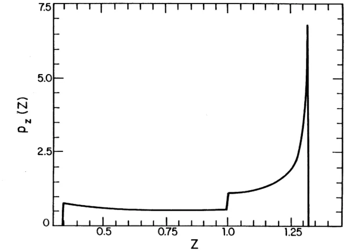
speckle targets... 61 4.2 Reflected phasefronts from glint targets... 64 4.3 Target return PDF for beam wander fluctuations,

Gaussian beam, uniform circular beam center,

|m/rb = 0.0, R/rb = 1.0 ... 77 4.4 Saturation SNR due to two types of beam wander

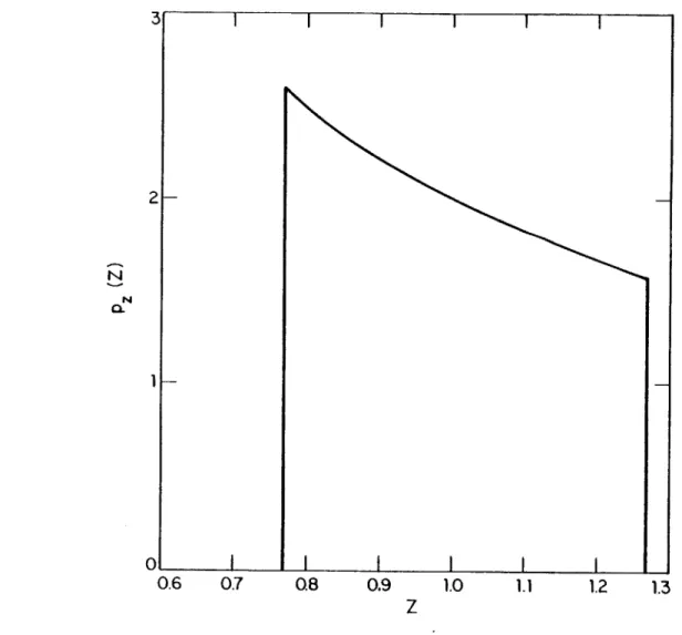
fluctuation... 78 4.5 Target return PDF for beam wander fluctuations;

fan beam, uniformly distributed beam center,

m/rb = .45, R/rb = 1.2... 82 4.6 Saturation SNR due to fan beam, uniform beam center

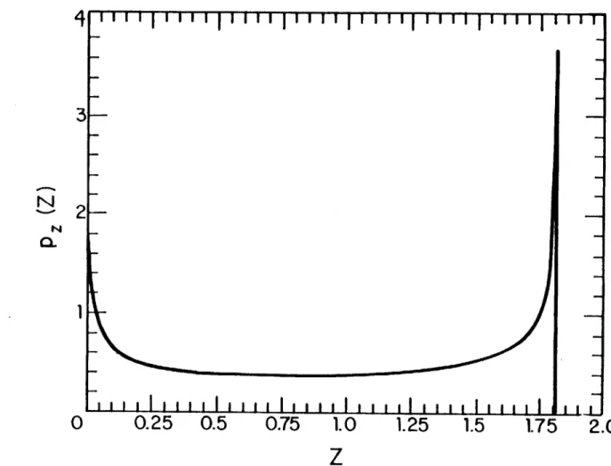
fluctuations... 83 4.7 Target return PDF for beam wander fluctuations;

fan beam, Gaussian distributed beam center, m/rb = 0.8, a /rb = 1.25... 85

LIST OF FIGURES Figure

4.8 Single scattering layer... 91 5.1 Normalized histogram of 100 consecutive retro returns

taken in full scanning mode and theoretical PDF

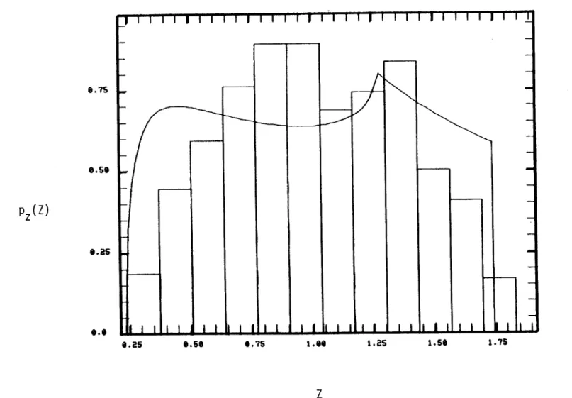
Eq. (4.F.23), R/rb = 1.3, m/rb = 0.0... 105 5.2 Normalized histogram of 200 consecutive returns taken in

full scanning mode and theoretical PDF Eq. (4.F.23),

R/rb = 1.2, m/rb = 0.5... 106 5.3 Normalized histogram of 200 consecutive retro returns taken

in full scanning mode and theoretical PDF (4.F.23),

R/rb = 1.3, m/rb = 0.56... 107 5.4 Normalized histogram of 200 consecutive retro returns from

the "side" pixel of Figure 5.2 taken in full scanning mode and theoretical PDF (4.F.28), R/rb = 1.2, m/rb = 1.43... 110 5.5 Normalized histogram of 400 consecutive retro returns

taken in full scanning mode and theoretical PDF (4.F.15),

R/rb = 1.4, m/rb = 0.6... 111 5.6 Normalized histogram of 100 "hot spot" retro returns

taken in reduced scanning mode and the lognormal PDF

(5.D.l), a2 _{= .0045... 114}

x

5.7 Time evolution; Row location of hot spot in the l00-60x128 pixel frames used in the example of Figure 5.6... 116 5.8 Time evolution; Column location of hot spot in the

l00-60x128 pixel frames used in the example of Figure 5.6... 117 5.9 Normalized histograms of 300 "hot spot" retro returns

taken in reduced scanning mode and the lognormal PDF

(5.D.1), a2 = 0.0138... 119 x

LIST OF FIGURES

Figure Pag

5.10 Normalized histogram of 400 "hot spots" retro returns taken in reduced scanning mode and the lognormal PDF

(5.D.1), &2 = 0.018... 120

x

5.11 Normalized histogram of 300 "hot spot" polished sphere returns taken in reduced scanning mode and the lognormal PDF (5.D.1), g2

= .0083... 121

x

5.12 Normalized histogram of 300 "hot spot" polished sphere returns taken in reduced scannina mode and the lognormal PDF (5.D.1), a'2 _{= 0.004... 122}

x

5.13 The theoretical curve (4.D.6) and estimates SNRSAT from

the data of Figures 5.6,5.9-5.12... 124 5.14 Normalized histogram of 2000 squared, consecutive

speckle plate returns taken in full scanning mode and

exponential PDF... 125 5.15 Normalized histogram of 400 consecutive speckle plate

returns taken in full scanning mode and Rayleigh PDF... 126 5.16 Normalized histooram of 1200 speckle plate returns

taken in reduced scanning mode and Rayleigh PDF... 128 5.17 Normalized histograms of 1400 consecutive speckle plate

returns taken in staring mode and Rayleigh PDF... 129 5.18 Normalized histogram of 300 speckle plate returns taken

in full scanning mode and Rayleigh PDF...131 5.19 Normalized histogram of the same 300 speckle target

returns as Figure 5.18 and a Rayleigh times lognormal

LIST OF FIGURES

Page 6.1 The probability density function, p (Y) = 2K (2VY)...142 6.2 Single pulse detection probability vs. CNR for a glint

target in bad weather...144 6.3 Single pulse receiver operating characteristics for a

glint target in bad weather...145 6.4 Single pulse detection probability vs. CNR for a single

glint target in free-space, three levels of turbulent

fluctuations and bad weather. P F = 10- throuhout...146 6.5 Likelihood ratio R (Eq. (6.C.3)) and parabola

log R = 3.1 + 0.3441r' vs, matched filter envelope

detector output Ir...149 6.6 Threshold y vs. number of pulses necessary to maintain

-=

102 154

PF

6.7 Single-pulse and multipulse detection probability vs. CNR for a glint target in bad weather. PF = 104 throughout.. 158 6.8 Single-pulse and multipulse detection probability vs.

CNR for a glint target in bad weather. PF=10-12 throughout. 159 6.9 The number of pulses M necessary to achieve PF = 10-12

pD= .99 vs. CNR for a glint target in free-space, two

turbulent fluctuation levels, and bad weather...160 6.10 The number of pulses M necessary to achieve PD = .99 and

two different false alarm probabilities vs. CNR for a

glint target in low visibility...161 6.11 Ten pulse detection probability vs. CNR for a glint

target in several turbulent atmospheres and a scattering atmosphere. PF = 10l2 throughout...163

LIST OF FIGURES

Figure Paae

6.12 Fifteen pulse detection probility vs. CNR for a glint target in several turbulent atmospheres and a scattering atmosphere. PF = 10-12 throughout...164 7.1 Geometry for a single scattering layer between radar

and target...170 7.2 Geometry for a scattering layer near the target...171 7.3 Normalized backscatter power from a uniform scattering

profile vs. t... ... 175 7.4 Maximum normalized backscatter power from a scattering

layer L meters from the radar...177 7.5 Extinguished free-space and MFS resolved speckle target

CNR vs. target range for the CO2 system and a uniform

scattering profile...178 7.6 Extinguished free-space and MFS resolved speckle target

CNR vs. tarqet range for the Nd:YAG system and a uniform scattering profile...179 7.7 Atmospheric beamwidth for a single layer scattering

profile vs. layer thickness...181 7.8 Extinguished free-space and MFS resolved speckle target

CNR for the CO2 system and a single scattering layer vs.

layer thickness...182 7.9 Extinguished free-space and MFS resolved speckle target

CNR for the Nd:YAG system and a single scattering layer

vs. layer thickness...183 7.10 Atmospheric beamwidth for a scattering layer near the

LIST OF FIGURES

Figure Page

7.11 Extinguished free-space and MFS resolved speckle target CNR for the Nd:YAG system and a scattering layer near the target vs. layer thickness... 187 7.12 Field coherence length for a scattering layer near the

target and the Nd:YAG system vs. layer thickness... 190 7.13 Extinguished free-space and MFS unresolved glint target

CNR for the Nd:YAG system and a scattering layer near

the taroet vs. layer thickness... 191 A.1 Geometry relating to the definition of specific

intensity... ... 198 A.2 Geometry for relating the specific intensity and the

mutual coherence function... 201 A.3 MCF's for plane wave input... 207 A.4 Real phase function... 209

LIST OF TABLES Table 7.1 7.2 7.3 7.4

CO_{2 Laser Radar System Parameters... 167}

Nd:YAG Laser Radar System Parameters... 168

Atmospheric Parameters at CO₂ Laser Wavelength... 172

Atmospheric Parameters at Nd:YAG Laser Wavelength.

Page

CHAPTER I

INTRODUCTION

The development of laser technology offers new alternatives to the problems of target detection and imaging. Among the advantages provided by laser radars over conventional radar systems are increased angular, range, and velocity resolution with compact equipment. However, performance of the laser system may be severely limited by the stochastic nature of atmospheric optical propagation; that is, by turbulence,

absorption, and scattering. Herein, a mathematical model describing a heterodyne reception optical radar is presented. The model incorporates the statistical effects of propagation through tubulent and turbid

atmospheric conditions, as well as target speckle and glint, and local oscillator shot noise.

A convenient theoretical model describing optical propagation through atmospheric turbulence has been established [1]. In contrast, optical propagation through bad weather is much more difficult to model and to date no comprehensive theory exists which characterizes this propagation regime in complete generality. From the available turbid atmosphere propagation models the multiple forward scatter (MFS) extended Huygens-Fresnel formulation [2] is useful in our application. Both the turbulence model and MFS model are expressed in linear-system form in which the random nature of the propagation process is represented by a

stochastic point source response function (Green's function). Such a linear model leads to a tractable overall radar system model.

In this thesis, we consider the performance of a scanning imaging system and to a lesser degree that of a target-detection system. By means of the turbulence model, the primary atmospheric effect limiting compact* radar system performance has previously been shown to be scintillation [3-5]. In contrast, beam spread and receiver coherence loss as well as scintillation will be shown to be important when the MFS model applies.

To validate the theory measurements made on the compact C02-laser

radar, developed as part of the M.I.T. Lincoln Laboratory Infrared Airborne Radar (IRAR) project, have been made available. The compact

laser radar system [6] employs a one-dimensional, twelve-element HgCdTe heterodyne detector, a transmit/receive telescope of 13 cm aperture, and a 10 W CO2, 10.6 vm laser, which is operated in pulsed mode. For each pulse, the intermediate frequency (IF) portion of the heterodyne detector outputs are digitally peak-detected to yield 8 bit range and intensity values. In the case of a large signal return the intensity value is essentially the output of a matched filter envelope detector. Hence, these data can be compared to the theory.

An outline of the topics covered herein is as follows. First, in this chapter, a description of the laser-radar configuration will be presented. This will be followed by descriptions of the atmospheric

*The term "compact" indicates a system that can be installed on a vehicle such as a truck or airplane.

propagation and target interaction models, which appear in Chapters II and III, respectively. The performance of a scanning-imaging radar in

both turbulence and low visibility will be considered in Chapter IV. As speckle target returns from disjoint diffraction-limited fields-of-view

(FOV) will be shown to be uncorrelated in low-visibility weather, and each picture element (pixel) of the image is assumed to encompass at least a diffraction-limited FOV, we need consider only single-pixel performance. This will be achieved via a signal-to-noise ratio (SNR) analysis. Also, speckle target resolution in bad weather is considered here. In Chapter V, theory verification efforts are described.

Single-pulse and multi-pulse target detection is explored in Chapter VI with emphasis given to low visibility results. In Chapter VII system examples are presented. Finally, in Chapter VIII, we summarize our results and present suggestions for future work.

A. Laser Radar Configuration

A model of the laser radar configuration is shown in Figure 1.1. A series of laser pulses ET(Pt) propagating nominally in the +z

direction are transmitted from the radar located in the z = 0 plane, and illuminate a target located in the z = L plane (Figure 1.la). A fraction of the illuminating field Et(PI',t) is reflected in the -z direction back towards the radar (Figure 1.1b). The nature of this reflected field

E r(',t) clearly depends upon the reflection characteristics of the target, as does the received field ER(p,t). This recieved field is mixed with a local-oscillator field E,(P,t) and focussed onto an optical detector. The

TRANSMITTER

TRANSMITTED

BEAM

FORWARD

PATH

ILLUMINATING

BEAM

ATMOSPHERE

RECEIVED

BEAM

b)

RETURN

PATH

REFLECTED

BEAM

TARGET

TARGET

Figure 1.1: Laser Radar Configuration

L

RECEIVER

A

TMOSPHERE

intermediate frequency (IF) component of the photocurrent comprises the observed signal.

To as large an extent as possible the analysis has been tailored to the IRAR project's compact C02-laser radar system. Thus, the

transmitter and receiver are taken to be co-located with common

entrance/exit optics of aperture diameter from 5 to 20 cm. The transmitter will be assumed to produce a periodic train of rectangular-envelope laser pulses while the local oscillator operates cw producing an ideal

monochromatic wave offset in frequency by the intermediate frequency v IF* Targets are assumed to lie along line-of-sight paths a distance L

from the radar where 1 km < L < 10 km. In accordance with the above

conditions and transmitter pulse durations and pulse repetition frequencies anticipated in real radar scenarios [7,8] we have the following

characterization.

1. The transmitted field has a quasi-monochromatic, linearly polarized electric field proportional to

ET(Pt) = Re{u (p,t) e 0 } (l.A.1) T

where v is the optical carrier frequency, and P = (x,y) is a position vector transverse to the direction of propagation. The complex envelope uT(P,t) is expressed as the product of a normalized spatial mode F(P) and a time waveform sT(t) whose magnitude square is the transmitted power PT(t) (Watts).

uT(P,t) = FT() -T(t) (1.A.2)

PT(t) = Is-T(t)12 (l.A.3)

dPIT( 12= 1 (1 .A.4)

This implies that 1u-T(P,t)I2 is the transmitted power density (Watts/m2). The transmitted power waveform PT(t) is assumed to be as shown in Figure 1.2 where t is the pulse duration and l/T the pulse repetition frequency.

2. We assume a scalar wave theory to describe the propagation. We also assume the pulse duration to be short in comparison

to an atmospheric coherence time Tc >> tp and long in

comparison to the reciprocal coherence bandwidth (multipath spread) of the atmosphere 1_/Bcoh

< t . The complex envelope of the illuminating field in the z = L plane can then be

represented by the linear superposition integral

ut(P',t) = dp hLF(PiP) T(p,t - L/c) (l.A.5)

where hLF(P'P) is the stochastic atmospheric Green's function (point source response) and c is the propagation velocity of light. The subscripts indicate a path length of L meters in the +z (or forward) direction. In free space (l.A.5)

PT (t)

0 t p T +t 2 , 2 c +

Pp p p p p p

hLF(PI',P) is random with statistical characterization dependent upon weather conditions.

3. A planar target-interaction model is assumed so that for a stationary target the complex envelope of the reflected field

is

I-r (PI',t) = ut (_',t) T(-') (l.A.6)

where T(P') is the field reflection coefficient at the point P'. In general T(p') is a random function containing

specular and diffuse components.

4. As before, we can represent the received field as a superposition integral

u (_gPqt) = d' h LR , ) -r(p',t - L/c) (l.A.7)

In (l.A.7) hLR(P,P') is aoain the stochastic atmospheric Green's function where the subscript R refers to propagation in the -z (or return) direction. In turbulence, and in low visibility when the target range is sufficiently short, the propagation medium is reciprocal [10,11], i.e.,

In low visibility and with a suitably large target range we take hLF and hLR to be statistically independent. This is due to the atmosphere decorrelating between pulse transmission and reception times, and is an appropriate assumption when the atmospheric coherence time Tc is shorter than the roundtrip propagation delay 2L/c. We will refer to the former case as "effectively monostatic" and the latter case as "effectively bistatic" regardless of the radar

configuration.

5. According to the antenna theorem for heterodyne reception [12], we can describe the photodetection process as though it were taking place in the receiver's entrance pupil. Thus, the detected field is taken to be ER(Pt) + EZ(p,t) where the cw field E, has complex envelope

j27rv

u(-,t) = P1 F (P) e IF (l.A.9)

In (l.A.9), vIF is the intermediate frequency, PZ the local oscillator average power and F a normalized spatial mode. The photocurrent is passed through a rectangular passband filter of bandwidth 2W centered at vIF. It is straightforward to show that under the strong local oscillator condition [13] a normalized (i.e. proportional to the photocurrent) IF signal r(t) can be expressed as filtered signal plus noise.

This is shown in Figure 1.3 where the pass band filter H(f) has the input with IF complex envelope

y(t) = _~hvJ

₀

-The additive noise n(t) is a zero-mean, white, circulo-complex Gaussian process with

<n(t) n*(s)> = tp 6(t - s) (l.A.ll)

where <-> denotes ensemble average, hv0 is the photon energy

and q is the detector quantum efficiency. Substituting for u_,t) in (l.A.10) and making the definitions

EF(I') d- h LF(PI',P) F T(P) (l.A.12)

P' = d h R ,1 )' *( ) ( .A.13)

the IF complex envelope (l.A.10) becomes

y(t) = 2 sT(t-2L/c) dF' T(P') EF R(P') + n(t) (1.A.14)

Re{y(t) e-} H(f) r(t) a) IF Model U' A H(f) 2W 2W -I I U

VIF

b) Normalized IF Filter Frequency Response

opposed to (l.A.10) which is performed over the receiver plane. From (l.A.10) it can be seen that to maximize signal return we should set F(p) = u (P)/( dpig(p)12) . In

practice, we set F,(P) = FT) to approximate this condition. In order not to block an appreciable amount of the signal return with H(f) we need 14 -1 1/t . To minimize the noise passed by the filter we set W = 1/t .

In both imaging and target detection applications the initial IF signal processing is identical. Namely, it is passed through a matched-filter envelope-detector with output proportional to

,2L/c+t~

mrij

= l/t

J

r(t) (Figure 1.3). In imaging, the scene is scanned and the complete image built up from sequential returns Fr| 2 separated in space typically by a diffraction limited FOV or more. In single-pulse detection ri2 is compared to a threshold where exceeding this threshold indicates

target presence. Optimal processing of returns for multi-pulse detection also requires knowledge of

Fr

CHAPTER II

ATMOSPHERIC PROPAGATION MODELS

The atmosphere, as an optical propagation medium, differs

markedly from free space. In clear weather, spatio-temporal refractive index fluctuations are caused by random mixing of air parcels of nonuniform temperatures. These fluctuations, called atmospheric turbulence, have a significant effect on optical propagation. In bad weather, scattering from aerosols, such as haze and fog, and hydrometeors, which include mist, rain and snow, can also profoundly affect propagation.

We anticipate three atmospheric propagation effects to degrade performance of the radar. Depending upon the relative sizes of the phase and amplitude field coherence lengths, transmitter and receiver apertures, and the target, different effects can become important. On a qualitative level we have:

1. Beam Spread. In the forward path, if the transmitter diamter exceeds the atmospheric coherence length p0, in either turbulent or low visibility weather, random dephasing of the transmitted field will occur. This results in a larger target plane illuminating beam than in free space.

In Figure 2.1 the field coherence length p = (1.09 k2 C2 L)-3/5

0 n

under clear weather conditions is shown versus path length L for three values of turbulence strength C2 and wavenumber k

n

101 X 10.6 p.m 1 2 5 x 101 m-2/3 n C= 5 x 10 m-n" 3 -2 2 3 45 10 10 10 10 L (i)

Figure 2.1: Turbulence field coherence length p0 vs. propagation path

length L for conditions of weak turbulence (C' = 5 x 10-16 m-2/3), moderate turbulence (C2 = 10-14 m-2/3), and strong turbulence

this digram we see that for typical transmitted beam

diameters of 5 to 20 cm and path lengths of 1 km to 10 km transmitter beam spread can nearly always be neglected. We will take this to be the case. On the other hand, for

turbid atmosphere propagation, the atmospheric coherence length p0 = ₀ (2/ s L 0' k_F 2)2 (see Appendix A), where S'

is the effective scattering coefficient and OF the forward scattering angle, generally is much smaller than typical beam diameters. Hence, as will be seen in more detail later, beam spread is an important factor in bad weather, and must be included in our analysis.

2. Scintillation. The random spatio-temporal amplitude fluctuations due to constructive and destructive

interference of the randomly lensed light is known as scintillation. If the target is smaller than the amplitude coherence length of the atmosphere then the scintillation modulates the reflected intensity. If the target is larger than this coherence distance the

scintillation presents itself as a speckling of the reflected radiation. In both turbulent and turbid atmospheres this effect is significant, although, we anticipate that signal return fluctuations will be of different character in the clear-weather and bad weather

3. Coherence loss. At the receiver, surfaces of constant phase will become wrinkled when the receiver aperture becomes larger than a phase coherence length (which is a numerical factor times p 0). When this occurs optimal spatial mode matching cannot be achieved with F*() = ET(p), resulting

in a performance degradation called coherence loss.

Referring to Figure 2.1, in turbulence, for typical receiver diameters of 5 to 20 cm and path lengths of 1 to 10 km this

effect can also be neglected. As coherence lengths in low visibility are normally much smaller than the receiver aperture this effect is pronounced. More details will be given later.

The above heuristic descriptions of propagation phenomena are lacking in mathematical detail. We now provide these details. First, free space propagation is described. Next, propagation through

turbulence is characterized. Finally, we discuss turbid atmosphere propagation.

A. Free Space Model

In free space reciprocity (Eq. (l.A.8)) applies with both hLF and hLR equal to the non-random Green's function [9]

where X is the optical wavelength, k = 27/X the wavenumber, and superscript "o" denotes free space.

B. Turbulence Model

Without loss of generality, the stochastic Green's function for the clear turbulent atmosphere can be represented as the product of an absorption term, a random, complex perturbation term and the free

space result [1,31

hL(P1,P) = e- aL/2 exp[x(T',W) + j(',P)] ho(-',-) (2.B.1)

where, via reciprocity, hL = hLF = hLR. In (2.B.1), a is the atmospheric absorption coefficient and x(I',-) ( (I',)) is the log-amplitude (phase) perturbation of the field at transverse

coordinate p' in the z = L plane due to a point source excitation at transverse coordinate P in the z = 0 plane. These perturbations, before the onset of saturated scintillation, may easily be expressed as sums of large numbers of independent random variables [1,14]. Hence, by the central limit theorem [15], x and c are jointly Gaussian random processes and completely characterized by their means and covariance functions. Such a complete characterization is provided in reference [1] but will not be given here. It will suffice to note that the mean log amplitude perturbation obeys m = -c2 as a result of energy

x x

conservation [16] where the log amplitude perturbation variance is given by

02 = min(O.124 C2 k7/ 6 L11/6,0.5) (2.B.2)

x n

for Kolmogorov spectrum turbulence with a uniform turbulence strength C2 profile.

C. Turbid Atmosphere Model

Again, without loss of generality, we can express the stochastic Green's function as a product form

hL(,) = e -a'L/2 A(',) exp[j (',P)] h0(P',) (2.C.1)

for either the forward or return path. This representation is chosen to emphasize that the amplitude perturbation A(p',p), and not its logarithm, is Gaussian. This results from the fact that nearly all of the light illuminating the target and receiver is scattered in bad weather. Hence, these fields are the sum of a large number of

independent contributions and, by the central limit theorem [15], can be taken to be Gaussian.

In Appendix A, the mutual coherence function (correlation function of the atmospheric Green's function hL) is derived. This is accomplished by considering scattering from a single particle and assuming: (1) single scattering is concentrated about the forward direction, (2) wide-angle scatter and back scatter can be lumped into absorption so that the real single particle phase function can be approximated by a Gaussian form, and (3) that L >> 1, where ' is the

modified atmospheric scattering coefficient, so that the direct

(unscattered) beam contribution to the field is insignificant compared to the scattered field.

The result we use is [2,17,18]

<hL (Til9 ) h*(p )> = e a exp[-(j ₂ +

IT'

-

(T1 _-P _2))/3pf] ho(TP ,p) h*( , 2 (2.C.2)

In (2.C.2), _aa'(> Ba) is the modified absorption coefficient containing

wide angle scatter and back scatter contributions and

Po= [L e2 k2 (2.C.3)

is the atmospheric coherence distance where e F is the root-mean-square forward-scattering angle of the Gaussian single particle phase function. Furthermore, the variance of the phase perturbation is large enough to say that hL(P',P) is zero mean and <hL(P',Pl) hL(' P2 )> =

The above model is known as the multiple forward scattering (MFS) approximation. The validity of the model is not fully

established. It should yield correct results when each scattering particle is significantly larger than a wavelength X. In this case,

the true single particle phase function would be highly peaked about

As discussed in Appendix A the correlation function (2.C.2) accounts only for scattered light. That is, results derived from (2.C.2) disregard the unscattered portion of the beam. In order to take this into account the unscattered beam is taken to be the

free-space result reduced by the extinction (absorption and scattering) loss. In this thesis, the main theoretical development is aimed at making use of the scattered light in the context of an optical radar. Clearly, before use can be made of the scattered power, as calculated via the MFS theory, it must dominate the extinguished free-space power. More will be said about this issue in Chapter VII.

D. Backscatter

When the monostatic radar, as described in Chapter I, is used in inclement weather there may be significant backscatter return from the hydrometeors and aerosols present in the propagation path. Clearly this return is undesirable in imaging and target detection applications, but unavoidable in such weather conditions. To see when such a

return can be significant its power must be compared to those of the MFS and extinguished free-space target returns. The backscatter

contribution to the radar return will be examined in Chapter IV, Section H and again in Chapter VII.

CHAPTER III

TARGET INTERACTION MODEL

Here we discuss how the reflected radiation is related to the target illumination. We first discuss the planar target model used in this analysis. This model is then related to the more usual bidirectional reflectance in the following section.

A. Planar Reflection Model

In scalar paraxial optics reflection of an optical beam from a spherical mirror is generally represented in terms of a planar

reflection model. If the incident and reflected fields travelling

nominally along the z-axis are noted ut (',t) and ur(P't), respectively, we have the relation

u- (I',t) = t(F',t) r expr-jkjp' -

1cf

where r is the intensity reflection coefficient, Rc is the radius of curvature of the mirror and p c is the transverse location of the center of curvature. The use of (3.A.1) presupposes -c lies on or near the

z-axis and Rc is much larger than the beamwidth of u-t More generally we might represent a polished reflecting surface by incorporating into

(3.A.1) spatially varying intensity reflection coefficient, radius of curvature and center of curvature. That is

ur(W',t) = ut(',t) r-

(')

I'

-

(P)I

would be our model. In accordance with (3.A.2) we shall assume that for all targets of interest a planar target interaction model (l.A.6) is applicable

Ur(I't) = u-t(p',t) T(P') (3.A.3)

In general, T(P') will contain two components, the so-called specular (glint) and diffuse (speckle) reflection components. We express this as

T(P') = eJO T (p') + Ts(p') (3.A.4)

The glint component, T (P'), is nonrandom and represents the component of the reflected liqht that is due to the smoothly-varying target shape. This component may be described by (3.A.2) or (3.A.1). The random

phase e is assumed to be uniformly distributed over [O,2tr] and represents our uncertainty of target depth on spatial scales on the order of a

wavelength. On the other hand, the speckle component T (_') is random and represents that part of the reflected light that is due to the microscopic surface-height fluctuations of the target. This component may be assumed to be a Gaussian random process with moments [19-21]

<T ( ')> = 0 (3.A.5)

<T (() ) Ts(T) )> = 0 (3.A.6)

-s 1 s 21

)6~

<TS a' _S )> = X Ts( ) 6( - ) (3.A.7)

Use of the above moments is justified by the fact that a purely

diffuse target would turn a perfectly coherent illuminating beam into a spatially incoherent reflected beam. The quantity Ts (p') can be interpreted to be the mean-square reflection coefficient at p'.

What is sought in operation of the radar is information about the target. In terms of the preceding model it is worthwhile to

mention what information we are seeking. We regard T(P') as the target. For the glint component we are interested in the field reflection

coefficient (P') while for the speckle component we want information on the mean-square reflection coefficient T(P'). Note that neither the random phase e nor the exact speckle component field reflection coefficient Ts(P') is regarded as interesting.

B. Relationship to Bidirectional Reflectance

Let us examine the relationship between the preceeding target statistical model and bidirectional reflectance, the target signature quantity that is generally measured [3,8,22]. For the target geometry

of Figure 3.1, the bidirectional reflectance may be defined as

(X; ₁ ; _r = _X21 _AT

<

plane wave exp(j27 i -p') then the total reflected field is given by exp(j2r 7 -p') T(p'). The portion of this reflected field that is in the fr direction is the function-space projection [23] of

exp(j2T i -P') T(I') onto the function exp(j27 Ir -p'), that is, the Fourier transform of the reflected field. Hence, the bidirectional reflectance gives the ratio of the average reflected radiance (W/m2sr) in the direction fR to the incident irradiance (W/m2) propagating in the direction .

REFLECTED FIELD U

r(U,+)

r

_

TA RG ET

Kiiiiiiii

fr

TARGET-PLANE FIELD

z

INEFFECTIVE PLANE OF INTERACTION

z

L

Figure 3.1: Geometry for defining bidirectional reflectance p'(x;Ti,Tr); the target plane field is chosen to be a plane wave of wavelength x propagating in the direction of the unit vector ii (Xfi is the projection of ij on the z = L plane); the radiance of the reflected field is measured in the direction of the unit vector ir (xfr is the projection of ir on the z = L plane).

CHAPTER IV

SCANNING-IMAGING RADAR ANALYSIS

With atmospheric propagation and target interaction models in hand we are ready to proceed with the scanning-imaging radar analysis. This will consist mainly of a signal-to-noise ratio (SNR) analysis. To a lesser extent resolution and correlation of simultaneous target returns are also considered.

We assume that an image is built up through scanning a scene diffraction-limited FOV by diffraction-limited FOV. With this kind of imaging system successive returns from the same direction are

separated in time typically by tens of milliseconds. Since atmospheric correlation times in both turbulence and low visibility are considerably shorter than 10 msec, successive returns can be taken to be independent. Accordingly, with the SNR definition given below, the N-pulse,

single-pixel SNR is N times the single-pulse SNR. Coupling this with the fact that speckle target returns from disjoint diffraction limited FOV's are independent when the MFS model applies, as shown below, the single-pulse SNR is a reasonable performance measure.

We begin this chapter with a formulation of the single-pulse SNR problem. In the following section, speckle target resolution in bad weather is considered. We then discuss how the various atmospheric degradation effects will be identified in the SNR formulas. Following

this, SNR results in turbulence and low visibility will be presented. We then explore the SNR degradation effects of beam wander due to

reset error in the radar aiming mechanism or atmospheric beam steering. Next, correlation of simultaneous returns from different directions is considered. Finally, backscatter from particles in the propagation path is examined.

A. Sinale Pulse SNR

We are interested in the target reflection strength and accordingly consider

2L/c ₊ tp

Ir12 = 1l/t J r(t) dt|2 _(4.A.1)

-2L/c

the output of a matched filter envelope detector with input r(t). Ignoring the passband filter of Figure 1.3 and assuming tp = 1/W (the tp second integration has approximately the same effect on the IF signal r(t) as the filter) we have

r12 _{= Ix +}

n12

(4.A.2)

where the signal return is given by the target plane integral

j'ft

pP T'~

_(4A3

x = d' T(p') G(p') s(i')i lyAen

of x, with moments <n2 > = 0 <In 2_> = 1 (4.A.4) (4.A.5)

Note that the normalization chosen in (4.A.3) leads to the simple result (4.A.5). The mean of the observation (4.A.2) is

_= 2> + <In12> _(4.A.6)

The term <In! 2> is signal independent and due to receiver noise. Hence, we define the image signal-to-noise ratio to be

(<lr2> - <ln2>)2 SNR = _ Var(I r12) <Ix 12>2 Var( I r12) (4.A. 7)

That is, the ratio of the square of the signal portion of the observation mean to the observation variance. Since n is zero mean complex-Gaussian with statistics (4.A.4), (4.A.5) it is straightforward to show

SNR = CNR/2

CNR/2 1

1_{SNR SAT 2CNR}

(4.A.8)

where the carrier-to-noise ratio (CNR) has been defined to be the ratio of the signal portion of the observation mean to the noise portion

CNR (4. A.9)

<tn_2>

and the saturation SNR is

<|x|2>2

SNRSAT = <I.X12> (4.A.10)

AT

Var(

)

For CNR 5 or CNR 2 (10 SNRSAT we can disregard the last term in the denominator of (4.A.8) and obtain

SNR = SNRSAT + CNR/2 SNRSAT (4.A.ll)

The maximum value of SNR is, from (4.A.ll), seen to be SNRSAT and is achieved when CNR >> 2 SNRSAT. Physically, this limiting SNR results when noise fluctuations become negligible in comparison to signal

fluctuations. From (4.A.8) and (4.A.ll) it can be seen that to complete the analysis we need to evaluate SNRSAT and CNR for a number of

atmospheric/target situations. In order to know these quantities we must calculate <tx!2> and Var(tx12). Direct calculation of <tx 2> via

the definition (4.A.3) is not too difficult but use of the same approach for Var(tx12_{), while in principle straightforward, yields results which}

quickly become unmanageable. A more reasonable approach is to try to develop a complete statistical characterization for Ix12 for a number of atmospheric/target scenarios. This approach, besides being simpler, has the advantage of providing the information needed for the target

detection problem. This is the approach to be taken.

Up to now no assumption has been made regarding the statistics of the signal return x. Therefore, the formulation of the imaging SNR problem in equations (4.A.1) to (4.A.ll) is equally applicable to free space, turbulence, and low visibility as well as beam wander induced fluctuations. To finish this section we give selected free space SNRSAT and CNR results.

Here we shall assume a Gaussian-beam system described by

FT(P) = F*(P) exp(_IP12/2p2) (4.A.12) (TrpTY

where PT is the radar transmitter and receiver pupil radius.

For a resolved speckle target (i.e. one that is larger than the illuminating beam size) with intensity reflection coefficient r in free space it is simple to show that

T.1P t 2TrP2

CNR = 0 r (4.A.13)

ho

L

and [3]

SNRSAT = 1 (4.A.14)

For an unresolved glint target, with field reflection coefficient

T (p ) = exp[- L' 1 2/2r 2] (4. A.15)

-<s

we have

CNR = 4rrsPTj L (4.A.16)

and a saturation SNR equal to infinity. More detailed examples of this type will be given later.

B. Speckle Target Resolution in the Low Visibility Atmosphere We consider the output of the matched filter envelope

detector (4.A.2) when the noise n is negligible so that

I

x(fT hjtp PT d-p' T(p) Eg p') Flp) (4.B.1)

and the, atmosphere is characterized by (2.C.2). In (4.B.1) we have explicitly noted that the signal return is a function of pulse propagation direction as defined by TT (-see below). Limiting

ourselves to pure speckle targets, the mean signal return < x(-T 2>

will be considered. In examining this quantity we will be concerned with what portion of the target contributes to the signal return.

Before giving the expression for the mean signal return it is worthwhile to develop some preliminary results. Namely, the field spatial correlation functions <F(Cj) gp)> and qR

should be found. For the resolution issues discussed in this section it is necessary to know these correlation functions only for p= p. The more general result ( 5 is useful in the sequel, though, and will be given here. To facilitate the calculations Gaussian transmitted and local-oscillator spatial modes are assumed

FT(P) exp[- I 2_/2 p2 + j2 T f-] (4.B.2) T (~TrP 2)T (T F*(P) -exp[-

P 1

R

In the above equations PT and PR correspond, respectively, to the transmitter pupil radius and receiver pupil radius and fT determines the direction of propagation as this pulse will illuminate a circular

region in the z = L plane centered on the transverse coordinates

P = ALfT.

The atmospheric Green's functions hLF(P',P) and hLR(PP') are taken to be statistically independent. This, as stated earlier, is the "effectively bistatic" assumption. In order for this assumption to be reasonable when the radar is in a monostatic configuration (i.e. when the transmitter and receiver are colocated) the roundtrip delay for

pulse propagation to the target and back to the radar must be longer than the atmospheric coherence time Tc. An upperbound on this coherence time [24,25] can be taken to be the time for a frozen atmosphere moving at the transverse wind velocity Vt to move a coherence distance p , i.e. Tc < P₀/Vt. This expression ignores random motion of the air molecules which could decorrelate the atmosphere much more quickly than the preceding expression would suggest. For T' = s'L = 10,

forward scattering angle eF = 10 mrad, 10.6 ym radiation and transverse wind velocity V t = 10 km/hr this upper bound on the atmospheric

coherence time is p₀/V t 25 psec. The roundtrip delay time td = 2L/c is 6.7 -psec at range L = 1 km so that delay is equal to the upper bound when range is approximately 3 km. Even with the maximum value for coherence time the "effectively bistatic" assumption can be made

for reasonable target- ranges.

The spatial modes (4.B.2), (4.B.3) and the definitions (l.A.12), (l.A.13) in combination with the moment (2.C.2) are used to develop

expressions for the field spatial correlation functions <L 4$>, <L 4>. To facilitate interpreting the results of later sections, the

atmospheric coherence distance p0 is taken to be different for the

forward and return paths. Specifically, poF replaces p0 in (2.C.2) for hLF(P',p) while poR replaces p0 for hLR(p',). Physically, such an

assumption is unreasonable for a monostatic radar and is made only to aid interpretation. The correlation functions are then given by

e 2 _exp[-p' TrrbF ALI 2/rbF - exp[-p |2_/rcF2 exp[j k

(p'

where for convenience we have expressed the result in sum and difference coordinates

(4. B.5)

(4.B.6)

In Equation (4.B.4) the beam radius rbF is

rbF = (AL/pF)2 + (AL/2TrpT)2 ₊

the coherence distance r cF is

(4.B.7) 2 2 bF "oF TT (AL/hrpOF)2 ₊ +(AL/2pT) + pT + rc = (4.B.8) <_-F( ') -LPF 2) -c = 1

(p

-

+

and the phase radius of curvature RoF is

4p + 3pF 2 rbF

R = L[T + bF (4.B.9)

oF P + 3p F r 2 T

The corresponding expressions for <-RC) L*(p)> are found from (4.B.4) - (4.B.9) by replacing pT by PR and PoF by PoR everywhere so that r F becomes rbR, rcF becomes r2R, and ROF becomes ROR.

Assuming the radar is "effectively bistatic," that it uses

the Gaussian spatial modes (4.B.2), (4.B.3) with PT = PR and poR= oF Po and that the target is pure speckle with moments (3.A.5) - (3.A.7),

the mean signal return is

< X( T)h T e-2 L x-- d~p' T (-P') exp[-Ip' - XLfT 2_{/r es} <'

0

is the target-plane resolution e~1 spot size. Equation (4.B.10) can be interpreted as saying the signal return is an average over a spot of

area r es centered at Lf If the target is in the radar's far field this becomes

rres 2 (XL/2mpT)2 _{[1 + ( T} (4.B.12)

which can be interpreted as saying that the signal return is an average taken over approximately 1 + 4/3 (p T/P)2 diffraction-limited fields of view.

C. Identification of Atmospheric Effects

Although we discussed earlier a number of atmospheric effects expected to degrade the performance of an optical radar, no indication was given as to how these effects might be identified in our performance analysis. Here we discuss how this identification will be made in the

SNR and CNR formulas to follow.

1. Forward-path beam spread loss. If PT is the transmitted

beam radius and p0 the atmospheric coherence distance, any

degradation due to beam spread in the forward path can be eliminated by letting PT become small in comparison to p0.

Under this condition diffraction would dominate any

atmospherically induced beam spread and this loss mechanism should be eliminated from the CNR and SNR formulas. Note that this approach will be useful only in interpreting low-visibility results as beam spread was already shown to be unimportant in turbulence.

2. Return path beam spread loss. After reflection of the illuminating beam the phase fronts of the return beam will undergo additional wrinkling and hence additional beam spread will be incurred. This source of beam spread loss is not

as easily identifed in the equations as the forward-path loss. But it should not be present when the target is pure speckle as the reflected light is effectively radiating into the 27r steradians solid angle in front of the target, nor should it be present when the target is pure glint and smaller than the coherence distance p as diffraction then dominates beamspread.

3. Receiver coherence loss. As this loss mechanism is due to a wrinkled phase front in the received field it can be eliminated by decreasing the receiver pupil radius PR to satisfy PR < Po. In this case, the received phase front will be flat over the receiver aperture and the spatial modes of the received and local oscillator fields will match. Coherence loss is not important in turbulence, as discussed earlier, so this approach is useful only in low visibility.

4. Scintillation. The effects of scintillation will be difficult to see in the CNR and SNRSAT formulas. These effects will become apparent when complete statistical characterizations of target returns are presented.,

We now proceed with a series of SNR, CNR examples corresponding to different atmospheric/target scenarios. Turbulence results will be presented first, followed by low visibility results.

D. Turbulence SNR Results

The results cited in this section have previously appeared in references [3-5,26]. They assume the Gaussian-beam system

(4.B.2), (4.B.3) with perfect transmitter, local oscillator mode matching Fp) = F*(p), PT = PR. We present these results as a series of examples.

Case 1. Turbulence, Unresolved Glint Target

Here a pure glint target T(p') = T (p') e

j

T (p') = F exp(-jkjp'-'|/Rc) p' -ALfT (4.D.l)

c_ c T d

and satisfies

Rc << L _(4.D.2)

(XRc 0 (4.D.3)

be shown that the effective radiating region of the target (4.D.1) (i.e. the region within the illuminated portion of the target that makes an appreciable contribution to the target return) has nominal diameter (R c)P. Hence (4.D.3) amounts to saying that the effective radiating region is smaller than an atmospheric coherence area. A target satisfying (4.D.l)-(4.D.3) is called a "single glint" target.

Furthermore, assuming that the target lies entirely within the illuminating beam, i.e. it is unresolved, we find that the signal return can be expressed as

-4cr 2

1x_1 2 = CNRgu e X exp[4X(p ,0)] (4.D.4)

where p' is the glint reflection point of (4.D.1) and exp[4X(',U)] is a lognormal random variable. In (4.D.4) CNRgu is the unresolved (denoted "u") glint (denoted "g") target, tubulent atmosphere

carrier-to-noise ratio and a2 _{is the variance of the log-amplitude}

X perturbatiort X( 9,9)

.

It follows from (4.D.4) that the single pulse image SNR satisfies

CNR /2

SNR u gu (4.D.5)

g 1 + CNR gu(e X - 1)/2 + 1/2 CNRgu

SNRSAT 1 (4.D.6)

SAT 16 a2

gu e X

If no turbulence is present, we have a2 0 and the saturation SNR X

(4.D.6) is infinite as predicted by (4.A.10). For a2 > 0, SNR

X gu

initially increases with increasing CNR until it reaches the scintillation-limited value (4.D.6). For cr2 > 1/16, SNRSAT is

X -STgu

severly limited by turbulence. Multiframe averaging is required to overcome this limit.

Case 2. Turbulence, Speckle Target

When the target is assumed to be pure speckle, T(p') = T ' the single pulse image SNR satisfies

CNR /2

SNRs 16 52 (4.D.7)

1 + CNR s[1 + 2(e X -1)C]/2 _{+ 1/2 CNRs}

where

C

4 P2 /XL

4T~ 2 _(4.D.8)

1 + 4 p T //L

in the weak perturbation regime and CNRs is the speckle (denoted "s") target, turbulent atmosphere CNR. If the mean-square reflection

coefficient T(p') does not vary appreciably over the region illuminated

by the radar (i.e., the target is resolved) the target return can be expressed as

Ix2 = CNRsr v e2u _(4.D.9)

where v is a unit mean exponential random variable and u is a Gaussian random variable, statistically independent of v, with mean -a2 and variance a2 _satisfying

2

1

e4c - 1 =

C(e

In (4.D.9), v represents the target speck The probability density function for the w = v e2u is given in [27]. If CNRs z 5,

standard form (4.A.ll) with

SNRSAT =

5As

6a2

X -

1)

(4.D.10)

le and u the scintillation. unit mean fluctuation

Equation (4.D.7) takes the

1

16 a2

1 + 2(e X -_1)c

(4.D.11)

From (4.D.11) note that SNRSAT < 1 with SNRSAT = 1 speckle limited saturation SNR.

For more details on turbulence SNR results, examples, the reader should see [3-5,26].

corresponding to

E. Low Visibility SNR Results

In this section first CNR and then SNR results will be developed for bad weather radar operation. Again, the Gaussian transmitted and local oscillator spatial modes (4.B.2), (4.B.3) as well as an atmosphere characterized by (2.C.2) are assumed. The correlation function (4.B.4) then applies to this case where we will

take the coherence distances for the forward and return paths to be different poR PoF* This will aid in interpreting the results of this section.

Assuming that the atmospheric coherence time Tc is short enough to justify saying the radar is "effectively bistatic" the CNR

(4.A.9) becomes

-nP t

CNR = Pt dpi dp <T(T ) T*(T)><-F ) L (Pj4

0

J

_(4.E.l)

Our task is now reduced to evaluating the integral (4.E.1). This is done as a series of examples, each corresponding to a different target. We will interpret the results in terms of the previously mentioned atmospheric degradation mechanisms.

Case 1. Low Visibility, Unresolved Speckle Target The target is pure speckle T(-') _-P = T (p') with_-S

Ts(P') exp[-I' 2

The mean square reflection coefficient _{Ts is Gaussian with width rs} and centered on the z axis. Although no real target would have the form (4.E.2) it is chosen to allow closed form evaluation of (4.E.1). Also the CNR results below would be applicable to any unresolved speckle target if we replace 7rr with the speckle target area AT. Assuming

rs<< rbF9rbR (4.E.3)

i.e., that the target is unresolved by the radar, the carrier-to-noise ratio (4.E.1) becomes

CNR = CNR0 exp[-2'L]

su su 1/3(XL/pOFTO 2 _{1/3(XL/p oR7} 2 _a

1 + 1 +

(XL/2T) 2 + p (XL/2rpR + R

*exp LTI2 (4.E.4)

rbF rbR/ rbF + rbR

where CNR 0 is the free space unresolved speckle target CNR su TIP t x2 r 2 CNR0 = T

_

The second multiplicative term in (4.E.4) is the forward-path beam spread loss since it approaches 1 as PT +* 0. Similarly the third term

can be identifed as the coherence-loss term as it approaches 1 as PR - 0. The fourth term represents absorption and the last gives the

loss due to the misalignment of the radar, i.e., that the center of the illuminating field is

IXLfT1

(XL/27rrpT) 2_{. At C0}

2 wavelength 10.6 ypm and transmitter pupil radius

PT = 6.5 cm, the change over from near field to far field occurs at approximately 2.6 km, midway through the expected useful range of the radar.

Case 2. Low Visibility, Resolved Speckle Target

The target is again pure speckle T(P') = T (-') with mean square reflection coefficient (4.E.2). Assuming

rs >> rbF, rbR (4.E.6)