Automatic Verification of Pipelined
Microprocessors
by
Vishal Lalit Bhagwati
Bachelor of Science, University of California at Berkeley (1992)
Submitted to the Department of Electrical Engineering and Computer
Science in partial fulfillment of the requirements for the degree of
Master of Science
at the
Massachusetts Institute of Technology
February, 1994
© Massachusetts Institute of Technology, 1994
n
vED-Signature of Author
Department of Electrical Engineering and Computer Science In December 9, 1993
I C'
Certified by
Accepted by
Srinivas Devadas Associate Professor of Electrical Engineering and Computer Science
0
. -Thesis Supervisor
I
"1t
jrederic
R. Morgenthaler Chairman, De artmen Commitet
on Graduate StudentsMAS
TI--C
Automatic Verification of Pipelined
Microprocessors
by
Vishal Lalit Bhagwati
Submitted to the
Department of Electrical Engineering and Computer Science
on December 9, 1993 in partial fulfillment of the requirements for the
degree of Master of Science.
Abstract
This thesis addresses the problem of automatically verifying large digital designs at the logic level, against high-level specifications. In this thesis, a methodology which allows for the verification of a specific class of synchronous machines, namely pipelined microprocessors, is presented. The specification is the instruction set of the microprocessor with respect to which the correctness property is to be verified. A relation, namely the -relation, is established between the input/output behavior of the implementation and specification. The relation corre-sponds to changes in the input/output behavior that result from pipelining, and takes into account data hazards and control transfer instructions that modify pipelined execution. The correctness requirement is that the -relation hold between the implementation and specifica-tion.
In this research symbolic simulation of the specification and implementation is used to verify their functional equivalence. The pipelined and unpipelined microprocessor are charac-terized as definite machines (i.e. a machine in which for some constant k, the output of the machine depends only on the last k inputs) for verification purposes. Only a small number of cycles, rather than exhaustive state transition graph traversal and state enumeration, have to be simulated for each machine to verify whether the implementation is in -relation with the specification. Experimental results are presented.
Thesis Supervisor: Srinivas Devadas
Acknowledgments
I benefited greatly from the work of Srinivas Devadas, my advisor, and Filip Van Aelten, who did ground-breaking work on using string function relations and symbolic simulation for behavioral verification. Professor Devadas helped me significantly during the frustrating moments of the research, and encouraged me to undertake difficult problems and solve them effectively.
I would like to thank the members of the 8ht floor VLSI group, my roommates, past and present, and friends for their extensive support during my work.
This thesis is dedicated to my father, who gave me the inspiration to give the best at what-ever I undertake, and whose fond memories will live with me forwhat-ever. Special thanks to mem-bers of my family for their continuing support to achieve my educational goals.
The work described in this thesis was done at the Research Laboratory of Electronics of the Massachusetts Institute of Technology.
Contents
1 Introduction
11
1.1 Context 11
1.2 Previous Work 14
1.3 The Work Described in This Thesis
16
2 String Function Relations
19
2.1 Introduction 19
2.2 Concepts and Notation
20
2.3 The "Don't care times" P-Relation
21
3 Automata Theoretic Verification Procedures
25
3.1 Introduction 25
3.2 Binary Decision Diagrams
26
3.3 Image Computation Using BDD's
28
3.4 Procedures for Verification of Finite State Machines
31
4 Microprocessors as Definite Machines for Verification
33
4.1 Introduction 33
4.2 Definite Machines
33
4.3 Verification Properties of Definite Machines and Microprocessors
34
4.3.1 Verification of Definite Machines
34
4.3.2 Microprocessors as Definite Machines
35
4.3.3 3-relation for Verification of Definite Machines
36
4.3.4 Verification of k-definite machines with variable k
39
4.3.5 Pipelined Microprocessors with Data Hazards
41
5 Verification of Pipelined Microprocessors using Symbolic Simulation
43
5.1 Introduction
43
5.2 Pipelined Microprocessors with fixed k
44
5.3 Pipelined Microprocessors with variable k
46
5.5 Verification of Pipelined Microprocessors with Interrupts
and Exceptions
49
5.6 Verification of Microprocessors with Dynamically Scheduled Pipelines
52
5.7 Verification of Superscalar Pipelined Microprocessors
54
6 Experimental Results
57
6.1 Introduction 57
6.2 VSM, a simple RISC processor
57
6.3 AlphaO, a simplified AlphaT M 62
7 Conclusion and Future Work
67
Chapter 1
Introduction
1.1 Context
Technological advances in the areas of design and fabrication have made hardware systems extremely large. As faster, physically smaller and higher functionality circuits are designed, in large part due to progress made in VLSI, their complexity continues to grow. This makes the design process long and tedious, and error prone. Computer-Aided Design is aimed at alleviat-ing these two major problems in the design process. The first problem is tackled with synthesis programs that automate certain design steps. The second problem is addressed by verification programs that allow a designer to verify the consistency between an initial specification and a derived implementation.
While much progress has been made in the area of synthesis, verification is still lagging behind. Simulation has traditionally been used to check for correct operation of hardware sys-tems, since it has long become impossible to reason about them informally. However, even this is now proving to be inadequate due to computational demands of the task involved. It is not practically feasible to simulate all possible input patterns to verify a hardware design.
Sym-Introduction
bolic simulation, where symbolic inputs are applied to cover a wider range of input and state space, is practiced increasingly as well. An alternative to post-design verification is the use of automated synthesis techniques supporting a correct-by-construction design style. Logic syn-thesis techniques have been fairly successful in automating the gate-level logic design of hard-ware systems. However, more progress is needed to automate the design process at the higher levels in order to produce designs of the same quality as is achievable today by hand. This leads to the need for independent verification procedures, and this need is recognized in indus-try.
There are compelling reasons for verifying hardware to be correct at the design stage, rather than after commercial production and the marketing stage. A comparatively recent alter-native to simulation has been the use of formal verification for determining hardware correct-ness. Formal verification is like mathematical proof. Just as correctness of a mathematically proven theorem holds regardless of the particular values that it is applied to, correctness of a formally verified hardware design holds regardless of its input values. Thus, consideration of all cases is implicit in a methodology of formal verification. We consider a formal hardware verification problem to consist of formally establishing that an implementation satisfies a
specification. The term implementation refers to the hardware design that is to be verified. This
entity can correspond to a design description at any level of hardware abstraction hierarchy. The term specification refers to the property with respect to which correctness is to be deter-mined. It can be expressed in a variety of ways - as a behavioral description, an abstracted structural description, a timing requirement etc. The implementation and the specification are regarded as given within the scope of any one problem, and it is required to formally prove the appropriate "satisfaction" relation [Gup92].
The ultimate task in verification is to demonstrate that a designed circuit has a correct behavior. Such a circuit can be very large, which makes it imperative that the verification pro-cedure be efficient. The verification task can be split in subtasks, and can be done hierarchi-cally. For instance, a first subtask may consist of demonstrating that a layout has a certain Boolean functionality (which can again be divided into extracting the transistor schematics
from the layout, and proving that the transistor schematic has a correct Boolean functionality). The remaining task is then to demonstrate that a logic design produces an intended overall behavior.
The intended behavior for a synchronous hardware design is not necessarily a specific input / output mapping. Circuits with different degrees of pipelining, or circuits with different degrees of parallelism, produce different input / output functions, but may all exhibit satisfac-tory input / output behavior. Behavioral verification addresses the problem of verifying that a circuit design exhibits a satisfactory input / output behavior [FVA92]. What constitutes a "sat-isfactory input / output behavior" depends on the domain of the application.
This thesis considers independent automatic verification of a class of synchronous
proces-sors, pipelined microprocesproces-sors, against behavioral specification. Pipelining is an
implementa-tion technique whereby multiple instrucimplementa-tions are overlapped in execuimplementa-tion. Today, pipelining is the key implementation technique to make fast CPUs [PH90]. The work to be done in an instruction is broken into smaller pieces, each of which takes a fraction of the time needed to complete the entire instruction. Each of these steps is called apipe stage. Thus pipelining takes advantage of instruction level parallelism to improve the throughput of the microprocessor. The throughput of the pipeline is determined by how often an instruction exits the pipeline. The pipeline designer's goal is to balance the length of the pipeline stages. If the stages are perfectly balanced, then the time per instruction on the pipelined machine - assuming ideal conditions (i.e. no stalls) - is equal to:
Time per instruction on unpipelined machine / Number of pipe stages.
Under these condition, the speedup from pipelining equals the number of pipe stages. The difficulty in designing pipelined microprocessors. arises due to control hazards, data hazards and event handling [PH90]. Complex pipelining techniques such as dynamic scheduling, superscalar pipelining, hardware branch prediction etc. are used to obtain maximum through-put in the microprocessor. The design and synthesis of such pipelined microprocessors are
Introduction
becoming automated, and computer-aided design tools are required to verify the correctness properties of such microprocessors.
1.2 Previous Work
Extensive work has been done on the verification of specific input / output mappings. Although this does not directly address the behavioral verification problem, it does so indi-rectly by providing procedures that can be used as building blocks in a behavioral verification system. Two classes of procedures have been developed for verifying that a circuit exhibits a specific input / output mapping: fully automatic procedures, and procedures that require user intervention. The second class is commonly denoted with the term "theorem-provers", which refer to methods of proving theorems. Theorem provers are built from a general purpose back-bone mechanism, which manipulates symbolic expressions by applying inference rules, searching for a way to derive a desired conclusion from a given premise. In contrast, automatic input / output verification procedures are built from representations and routines that are spe-cifically tailored to the problem at hand. Many of the achievements in theorem proving tech-niques are being superceded by recent advances in automatic procedures. However, theorem proving techniques, such as in [Hun85], [Coh88] and [Joy88]), do have strengths that can be used to advantage for verifying large circuits, namely the allowance for functional abstraction
and proof by induction, but they typically require extensive user interaction.
Procedures for verifying strict input / output equivalence between two Finite State Machines (FSMs) were introduced in [CBM89] [Bry87]. This involved exhaustively travers-ing the State Transition Graph of the product of the two machines, ustravers-ing implicit state enumer-ation techniques. These are also known as symbolic simulenumer-ation techniques. In symbolic simulation, the input patterns are allowed to contain Boolean variables in addition to constants (0, 1, and X). Efficient symbolic manipulation techniques for Boolean functions allow multi-ple input patterns to be simulated in one step, potentially leading to much better results that can be obtained with conventional exhaustive simulation. This makes the hardware verifica-tion problem, which is NP-hard in general, more tractable and therefore attractive, in practice.
A way of formalizing behavioral equivalence is through string function relations, intro-duced by Bronstein [Bro89]. Both the implementation and specification are taken to be syn-chronous machines which have unique string functions associated with them. These string functions map sequences (strings) of input values into sequences of output values. Behavioral equivalence is modeled as a relation between two string functions. Bronstein defined two rela-tions other than strict input / output equivalence: the a- and P-relarela-tions, capturing delay and stuttering due to pipelining respectively. Bronstein used the Boyer-Moore theorem prover for the verification of these relations. This allows for the verification of possibly large designs, but
requires sophisticated and extensive user interaction.
Sequential logic verification procedures have been extended to allow for differences in the input/output behavior of the specification and implementation by Van Aelten et al [AAD91] [FVA92]. A relation is established between the input/output behavior of the implementation and specification using string function relations. The relation corresponds to changes in the input/output behavior that frequently result from a behavioral or sequential logic synthesis step. It is then possible to automatically verify whether the implementation satisfies the rela-tion with the specificarela-tion. The definirela-tion of the 3-relarela-tion is extended to general pipelined processors in [FVA92], and the a-relation is subsumed within the extended 5-relation. Sym-bolic simulation methods based on automata theory are used to verify the p-relation. The cir-cuit examples used in this work are those associated with digital signal processing.
A method for verification of pipelined hardware is described by Bose and Fisher [BK89]. They describe a symbolic simulation method for verifying synchronous pipelined circuits based on Hoare-style verification [Hoa69]. To deal with the conceptual complexity associated with pipelined designs, they suggest the use of an abstraction function, originally introduced by Hoare to work with abstract data types [Hoa72]. Given a state of the pipelined machine, the abstraction function maps it to an abstract pipelined state. Behavioral specifications for this abstract state space are given in terms of pre- and post-conditions, expressed in propositional logic. By choosing the same domain for the abstract states as the circuit value domain, they are able to automate both the evaluation of the abstraction function as well as verification of the
Introduction
behavioral assertions. Their technique is demonstrated on a CMOS implementation of a sys-tolic stack. The actual circuit provides inputs to the "abstraction circuit", and the assertions are verified at the abstract state level by a symbolic simulator.
1.3 The Work Described in This Thesis
The work described in this thesis focuses on independent behavioral verification of a class of synchronous machines, namely pipelined microprocessors. In my approach, the implementa-tion to be verified is a pipelined microprocessor, and is described in a high-level language sim-ilar to BDS [Seg87]. The specification is the instruction set of the microprocessor with respect to which the correctness property is to be verified. It corresponds to an unpipelined implemen-tation of the same instruction set, and is also described in BDS. Logic implemenimplemen-tations of these descriptions can be synthesized using a program similar to BDSYN [Seg87]. The cor-rectness requirement is that a P-relation holds between the implementation and specification. The p-relation relates a circuit, that processes inputs at certain relevant time points, and pro-duces outputs at certain relevant time points only, to a circuit of similar functionality that takes and produces relevant inputs and outputs at all time points.
My strategy of verifying the functionality of the implementation against that of the specifi-cation involves implicit state enumeration techniques as described in [CBM89]. The pipelined and unpipelined microprocessor are characterized as definite machines (i.e. a machine in which for some constant k, the output of the machine depends only on the last k inputs) for ver-ification purposes. In Chapter 4 it is shown that only a small number of cycles, rather than exhaustive traversal, have to be simulated for each machine to verify correctness using the
3-relation. The -relation can be used to model changes in pipelined execution due to data haz-ards and control transfer instructions. A derivative of the 13-relation, the dynamic p-relation is developed to verify complex pipelined structures such as interrupt handling, dynamic schedul-ing, and superscalar pipelines. This makes our methodology viable for large digital systems with complex pipelines.
The thesis is organized as follows. Chapter 2 contains preliminaries on the theory of string function relations. Chapter 3 describes automata theoretic symbolic simulation methods for synchronous machines. In Chapter 4, microprocessors are characterized as definite machines, and their properties that are essential for verification purposes are stated and proved. Chapter 5 contains the methodology used for verifying the pipelined processor implementation against the unpipelined specification. Verification of advanced pipeline structures, such as interrupt handling, superscalar pipelines, and dynamic scheduling are also described in Chapter 5. In Chapter 6, preliminary experimental results are presented. Chapter 7 contains conclusions of the research and gives directions for future work in this area.
Chapter 2
String Function Relations
2.1 Introduction
There are two fundamental ways of describing deterministic sequential machines with func-tions. One way is a function taking inputs and present states and producing outputs and next states. The other way is with a function taking a sequence (string) of inputs and producing a sequence of outputs, which describes the behavior of a sequential machine for a given initial condition as described in Bronstein's thesis [Bro89]. Both models have particular merits. The first model is indispensable for implementing a circuit, and is useful for many manipulations in the design process, since it is finite. The second model captures more directly the input / output behavior of a circuit, and is useful for expressing and proving certain properties, but since it is infinite (it is a mapping from arbitrarily long input streams to equally long output streams), it seems to be poorly suited for mechanical manipulations. I use both models in my thesis. The string model is used to define behavioral relations between sequential machines, and to prove certain properties of these relations by hand. The operational level is used for the bottom-level mechanized verification work.
String Function Relations
This chapter presents the formal correctness requirement we verify, in the form of a rela-tion between the implementarela-tion and the specificarela-tion. The relarela-tion corresponds to changes in the input/output behavior that frequently result from a behavioral or sequential logic synthesis step. Formally, we take both the specification and implementation to be synchronous machines and consider the string functions realized by each of them.
This chapter presents string functions and relations between them. Section 2.2 introduces strings, string functions, and notation, as they were presented in [Bro89]. Section 2.3 presents the "don't care times" relation, also known as the P-relation for synchronous machines. Other primitive relations such as the parallelism relation (y), the encoding relation (8), the input don't cares relation (), the output don't cares relation (0 are described in detail in [FVA92].
2.2 Concepts and Notation
Consider an alphabet E of values that can appear at the input and output ports of a syn-chronous circuit. Strings can be defined as finite concatenations of characters in the alphabet. Formally, the set of strings, E*, is defined as u(i)ieW where w is the set of all natural numbers including 0. We use variables u, v, ... for characters, and x, y, ... for strings. The empty string is denoted by e. Useful operations on strings are as follows:
.: Concatenate: f: x v -- C*, concatenate two strings (or a string and a character), the sec-ond string to the right of the first string. Sometimes the "." will be omitted.
*I
: Length: Z* -e w, a length of the string.· : Prefix: E* x * {TF), prefix relation on strings.
Defined by: (x < eX x = ) and (x < y.u x = y.u orx < y).
*L: Last:
E*
e l. the last character of the string.Defined by: L(x.u) = u (and L(e) = e for totality).
Defined by: P(x.u) = x and (P(e) = e for totality).
* t:
To the power: I x w - Y.*, which takes a character and a number n, and returns n repeti-tions of the character,* 1: At position: l;* x w - X, which takes a string and a number n, and extracts the nth charac-ter from the string. We will use xli.j as an abbreviation for the string (xi) ... (xJ).
Synchronous systems are constructed from two kinds of building blocks: combinational blocks, implementing a string functionf, the string extension of a character functionf, and registers, which implement a register function Ra that inserts a character a to the left of an input string and cuts off the right most character (Ra(x.u) = a.x and Ra(e) = £).
It is formally demonstrated in [Bro89] that synchronous systems, composed from these primitives, in which every loop contains a register, have a unique associated string function from Y* to 1*. Such systems are denoted as SF, SG, etc., and the corresponding string functions with F and G. It can be seen that these string functions are length preserving (the output string has the same length as the input string) and prefix preserving (if x is a prefix of y, the image of x under the string function is a prefix of the image of y).
As in [Bro89], Greek letters are used for relations between string functions realizable by synchronous machines. For example, F p G means F is in p relation with G. The "don't care times" n-relation is of interest to us, and is discussed in Section 2.3.
The alphabets of interest to us contain vectors of Booleans of some length. 0 is used both for the scalar 0 and for vectors containing all O's. zero is the string function taking arbitrary strings x and returning 0T I x . Likewise for 1 and one.
2.3 The ":Don't care times" P-Relation
Consider an implementation and a specification, both of them being synchronous systems,
SF and SG respectively, with corresponding string functions F and G. An implementation is
String Function Relations
functions of the two machines. The relation verified in this thesis is similar to the "don't care times" relation, 3, which is defined in [AAD91]. This section presents a formal definition of the B3-relation.
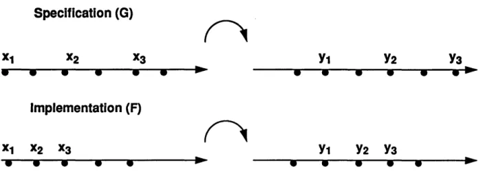
Specification (G)
X2 --x
3 p pImplementation (F)
x1 x2 x3 * * p Y1 Y2 Y3 Y1 Y2 Y3*
.
a ·
-
a
p pFIGURE 1. The
(-relation
between F and GThe "don't care times" relation relates implementation / specification pairs such as the one illustrated in Figure 1. The specification ignores input values at certain time points, and pro-duces irrelevant outputs at certain time points. In addition, the output stream of the implemen-tation is delayed with respect to the one of the specification.
To define the (3-relation, a function Relevant, which selects the relevant values in a string, i.e. omits the ones at "don't care times", has to be defined first.
Definition 23.1 (Relevant): f*x B* - *: Relevant(e,e) = e Relevant(x.u,y.v) = Relevant(x,y) ,v = 0 = Relevant(x,y).u ,v =
1
x.
U. -- g po 1r_"11
The symbol x represents the string Cartesian product, which combines strings of equal length. The Relevant-function takes a string over an arbitrary alphabet and a Boolean valued string, and returns what remains of the first string after deleting all values for which there is a 0 in the corresponding place in the Boolean valued string.
Let G be the specification and F be an implementation. Let H be a function that filters out the relevant outputs from F and G for verification. Let n be the delay between the output streams of F and G. Then the [-relation is defined as follows.
Definition 23.2 ([-relation):
Let H be a length and prefix preserving string function from E* to B*, realizable by some synchronous machine.
F PH, G = xe Y* s.t.
IxI
n,
Relevant (F(x), Rotn o H(x)) = G (Relevant (xl...(I x I -n), H(xJll...(Il x I - n)))).
This definition says that string functions F and G are in [3-relation if applying F to an input stream x, and then picking out the relevant output values, gives the same result as applying G to the relevant input values only. Figure 1 gives an example of applying the [3-relation. Here H is a modulo-2 counter and n=l.
Because of the delay of the output stream of the implementation, the filtering function H in the left-hand side of the identity has to be delayed over n cycles. In the right-hand side, the last
n characters of the input string have to be eliminated to make the left-hand side and the
right-hand side strings of equal length.
Design examples where don't care times occur are:
*A pipelined CPU which has delay slots when taking a branch. Because of the pipelining, not enough information is available for timely execution of a conditional branch. By default the branch is not taken, and when it later appears that the branch should have been taken, the pipeline has to be purged during a number of clock cycles. The outputs produced at those
String Function Relations
clock cycles are irrelevant. Moreover, for verification of a pipelined CPU versus an unpipe-lined CPU, the outputs produced by the unpipeunpipe-lined CPU at certain time points may be irrel-evant when comparing outputs with the pipelined CPU at those time points.
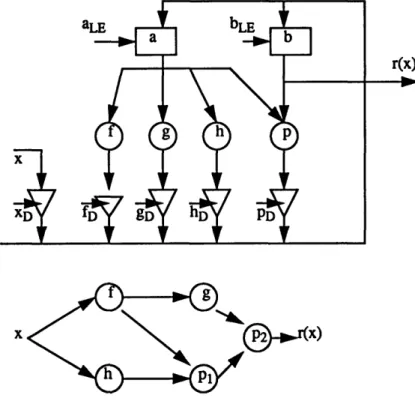
*Implementation / Specification pairs as shown in Figure 2. The controller of the implemen-tation is not shown. It repetitively sequences through six states, performing all of the opera-tions of the specification serially. (Taking an input is also considered as an operation.)
x
FIGURE 2.Example of an implementation and specification which are in 13-relation
The "don't care times" relation is inspired by the stutter-relation in [Bro89], but is slightly different. The (a-relation was defined in [Bro89] in the following way:
F G z' I I z I = Iz' I , V x E , F(x.z')= z.G()
It is almost subsumed by the 1-relation. If only the delay of F with respect to G is impor-tant, and not the characters in z, then F Pone, I z I G is equivalent to F alzl G.
Chapter 3
Automata Theoretic Verification
Proce-dures
3.1 Introduction
This chapter presents an elementary procedure for verification of finite state machines, based on the finite-automaton model. It verifies the input / output equivalence of two deterministic finite state machines. This procedure entails a traversal of the state transition graphs of each machine.
For equivalence checking, a product machine is constructed from the two machines, which produces an output of 1 if and only if the two machines agree on a given input. The transition graph of the product machine has to be traversed to see if all states under all input combina-tions is produce an output of 1.
There are a number of strategies for traversing a state transition graph. Starting from a cer-tain state, the input combinations leading to a transition out of the state can be enumerated explicitly (i.e. one by one) or implicitly (i.e. in sets). Likewise, the states in the transition graph can be enumerated explicitly and implicitly. For implicit enumeration, different
repre-Automata Theoretic Verification Procedures
sentations can be used for sets of input combinations or sets of states (e.g. cubes, sum-of-prod-ucts, binary decision diagrams). Finally, the traversal can be done depth-first or breadth-first. The methodology that is developed in this work does not commit to any one approach, but the experiments are done with implicit input and state enumeration, based on BDDs, with breadth-first traversal. This is currently the most robust and applicable technique.
Section 3.2 presents the binary decision diagram (BDD)-representation for Boolean func-tions. Section 3.3 presents image computation routines, for computing the set of states reach-able in one step from a given set of states under certain input conditions. These procedures perform implicit input and state enumeration, using BDD's, and can be used for breadth-first traversal. In Section 3.4, a FSM verification procedure is introduced which is used for the methodology developed in this thesis.
3.2 Binary Decision Diagrams
A binary decision diagram (BDD) for a functionf(xl, x2, x3,.... x) is a graph with
non-termi-nal vertices annotated with input variables, and terminon-termi-nal vertices annotated with a constant 0 or 1. Figure 3 gives an example of a BDD. All non-terminal vertices have one or more parent vertices and two children vertices, except for the unique root vertex, which has no parents. The terminal vertices have one or more parents and no children. The two edges going down from a non-terminal vertex to their children are annotated with a 0 and a 1. For a given assignment to the input variables xi, one can go down the decision diagram choosing -edges where a vari-able has a value 1, and O-edges where a varivari-able has the value 0. The value of the terminal ver-tex is the value off under the input combination.
An ordered BDD is one where the ordering of the variables is the same along any path
from the top vertex to a terminal vertex. A reduced BDD has no vertex which has a 1- and 0-edges pointing to the same vertex, or pointing to isomorphic subgraphs. The example BDD in Figure 3 is both ordered and reduced. Reduced Ordered BDDs (ROBDDs) were introduced in [Bry86]. They have a number of properties that make them very well suited for verification. Foremost is the fact that they are canonical, so that equivalence checking between two
func-tions is done by checking for isomorphism between the corresponding BDD's which requires linear time.
FIGURE 3.Reduced ordered binary decision diagram representing f = xlx3 + xlx2x3
It is not necessary for a Boolean function representation to be canonical to be suitable for equivalence checking. An alternative way of checking equivalence is to apply the XOR-func-tion to the outputs of both funcXOR-func-tions, and to check for satisfiability of the resulting funcXOR-func-tion. Both operations can be efficiently performed with BDDs. Satisfiability checking requires con-stant time, and applying a Boolean function to two BDDs requires time proportional to the product of the sizes of the BDDs to which the function is applied.
The apply-operation is also used to construct the BDD for a given implementation of a logic function. Starting from the primary input variables (for which the BDDs are trivial), Boolean functions AND, OR, XOR, XNOR, etc. are applied to BDDs of subfunctions, until a BDD is obtained for the function corresponding to the implementation's output.
The apply-operation can be performed recursively as follows. To compute fl<op> f2, given ROBDDsfj andf2 with top vertices vl and v2 respectively, do the following:
1. If vl and v2 are terminal vertices, generate a terminal vertex annotated with value (vl) <op>
Automata Theoretic Verification Procedures
2. If v1and v2 are annotated with the same variable, construct a vertex annotated with the
vari-able, having as O-child the result of applying <op> to the O-children of vl and v2, and as
1-child the result of applying <op> to the 1-1-children of vl and v2.
3. If the variables are different, or if one vertex is a terminal vertex, construct a vertex anno-tated with the variable coming earliest in the variable ordering (i.e. the one that has to appear first along any path from top to terminal vertex). Say that this variable corresponds with v1. Give to the constructed vertex as O-child the result of applying <op> to v2 and the
O-child of v1, and as -child the result of applying <op> to v2 and the 1-child of v1.
The size of the ROBDD is critically dependent on the ordering of input variables. To obtain small BDDs, the variables have to be ordered in such a way that assigning values to the first m input variables (0 < m < n) can, for the purpose of computingf, be "remembered" with less information than the detailed assignment (which can take 2m different values). For
exam-ple, for computing the sum of two integers represented as bit vectors, it is advantageous to interleave the two input vectors, and order the bits from lowest order to highest order. In that case, the only information to be "remembered" from an assignment to the lower order input bits, for the computation of the higher order bits, is one carry-bit.
Such variable orderings are not always feasible. For instance, it has been shown that an ROBDD for a multiplier takes 1(1.09n ) space regardless of the variable ordering [Bry91]. Most other practical Boolean functions, however, can be represented efficiently as an ROBDD.
3.3 Image Computation Using BDD's
Image computations constitute the core of the verification procedures to be discussed in Sec-tion 3.4. The following is the problem of image computaSec-tion:
Letfbe a function from Bn to Bm, where B = (0,1 . LetA be a subset of Bn. ComputeftA), the image of A underf, defined as y E Bm
I
3x E Bns.t. y =f(x) .An elegant method for image computation is the transition relation method, introduced in [CBM89] and is used for the experiments in this thesis. It works with a BDD representation of the transition relation R corresponding to the functionf. The transition relation maps inputs from Bn+m into B. It produces an output of 1 if and only if the vectory composed of the last m inputs and the vector x composed of the first n inputs are such that y =ffx).
Subsets A of Bn are in one-to-one correspondence with functions from Bnto B. The
char-acteristic function of a set A is a function that returns 1 if and only if the input is an element of
A. The symbol A is used for characteristic functions as well as for sets. Likewise,ffA) is used
for characteristic functions and sets.
The image offlA) consists of y-vectors such that there is an x-vector for which both R and
A are 1. The existential quantification can be computed with the smoothing operator, which is
defined as follows.
Definition 33.1 (Smoothing Operator)
Letf Bn - B be a Boolean function, and x = (xil, ... , xi5) a set of input variables off. The smoothing off by x is defined as:
Sxf = Sil f... Sxikf
Sxijf=fxij
+fij
In this definition fa designates the cofactor off by literal a. For instance fij isf with xi restricted to be 1, andfj isf with xii restricted to be 0. It can be seen that
(3x
I
R(x,y) ^ A(x)) SxR(x,y) . A(x))and therefore
f(A)(x) = Sx(R(x,y) A(x))
Cofactoring with respect to a literal is a trivial operation on BDDs. For instance, cofactor-ing by xi is done by deleting the xi vertices and attaching their -children to their parents,
Automata Theoretic Verification Procedures
reducing the resulting BDD if necessary. Applying OR- and AND- operations can be done as explained in Section 3.2.
Given the transition relation A(pit, pst, ns') and a set of states Cips), the next set of states
Ci+l(ps) can be calculated as follows:
Ei(ps, ns') =
I r
C(ps) n A(pit, ps:, ns')C'i+l(ns') = Sps Ei
ci+l(ps) - C'i+l(ps)
u Ci(ps)
where pit are the set of primary inputs, pst are the set of present state lines, and ns'tare the
transition relation inputs, and A(pit, pst, ns't) = 1 if state nst reached on applying pitto pst is
ns't = nst.
The smoothing and AND-operation can be performed simultaneously [BCMD90]. The resulting procedure has the same recursive and case-structure as the one for the apply opera-tion. The only difference occurs when the variable corresponding to a newly constructed top vertex has to be smoothed away. In that case the OR of the left child and the right child is com-puted. This operation is recursive in itself.
The transition relation method can also be used for inverse image computations, where outputs y are given, and inputs x have to be found such thatfAx) = y.
An alternative method for image computations, making use of Boolean functionf only, and not the transition relation R, was introduced in [CBM89]. This method can only be used for forward image computations, not for inverse ones. A good exposition of the method, as well as an extensive set of experimental results, can be found in [TSBS90], which reports that the transition relation method was superior for all the test cases considered.
3.4 Procedures for Verification of Finite State Machines
Using the method described above for image computation, one can check the input / output equivalence of two FSM's. First, construct the product machine, consisting of the original machines with corresponding outputs feeding XNOR gates, and the XNOR gates feeding one AND gate. The product machine is such that it produces an output of 1 if and only if the two component machines agree on a given input.
Second, compute the set of reachable states of the product machine by iteratively comput-ing sets Ciuntil Ci+l = Ci. Let so be the initial state of the machine, I the set of inputs under
which we need to find the set of next states, andf the next state function.
Co = (so'l
Ci+ = Ciuf(C ix I)
Ciis the set of states that can be reached in i or fewer steps. The final C, (which is equal to Cn
1) constitutes the set of all reachable states.
With g being the output function, the two machines are equivalent if and only if g(Cn x I) is a tautology.
Chapter 4
Microprocessors as Definite Machines
for Verification
4.1 Introduction
In this chapter, the concept of definite machines is introduced as described in [Koh78]. While the behavior of some synchronous machines depends on remote history, the behavior of others depends only on more recent events. The amount of past input and output information needed in order to determine the machine's future is called the memory span of the machine.
Section 4.2 introduces the concept of definite machines, for which only a small amount of past input information is needed to determine the machine's output. Section 4.3 describes cer-tain properties of definite machines that are essential for verification purposes, and these prop-erties form the most important theoretical basis for the efficient verification methodology described in this thesis.
4.2 Definite Machines
Microprocessors as Definite Machines for Verification
A sequential machine M is called a definite machine of order R if AX is the least integer, so that the present state of M can be determined uniquely from the knowledge of the last g inputs to M.
A definite machine has finite input memory. On the other hand, for a nondefinite machine there always exists at least one input sequence of arbitrary length, which does not provide enough information to identify the state of the machine. A definite machine of order IA is often called a -definite machine. If a machine is Ix-definite, it is also of finite memory of order equal to or smaller than pg.
The knowledge of any p. past input values is always sufficient to completely specify the present state of a gI-definite machine. Therefore any gI-definite machine can be realized as a cascade connection of pg delay elements, which store the last R input values, and a combina-tional circuit which generates the specific output. This realization, which is often referred to as
the canonical realization of a definite machine is shown in Figure 4. A more detailed treatment
of definite machines is given in [Koh78].
4.3 Verification Properties of Definite Machines and Microprocessors
4.3.1 Verification of Definite Machines
Theorem 4.3.1.1 Given two g-definite machines, let r be the number of possible inputs to each g-definite machine. Then the two gI-definite machines can be verified with X9 sequences
of length p.
Proof:
We know that the present state of a g-definite machine can be uniquely determined from the last g inputs. Since the number of possible inputs is x, the number of all possible permuta-tions of inputs sequences of length is i&. These sequences will enumerate all the unique states of each of the g-definite machines and the corresponding outputs. If the enumerated states and outputs of the two machines are equivalent, then the two machines are functionally equivalent for the set of ng input sequences.
Machine M
X I X2 X X
CL
FIGURE 4.Canonical Realization of a g-definite machine
If the machines are not functionally equivalent even if n[t sequences of length P produce equivalent present states and outputs of the two machines, then there exists a sequence of length greater than g which produces a different present state or output, or does not provide enough information to identify the state of either machine. But then it would make the machine nondefinite and with non-finite input memory. This is a contradiction to the original assumption of having g-definite machines.
Thus the claim holds true, and two g-definite machines can be verified with ['t sequences
of length g. O
4.3.2 Microprocessors as Definite Machines
We argue in this section that a microprocessor, pipelined or unpipelined, can be approximated as a definite machine for verification purposes.
A pipelined microprocessor is designed to have k pipeline stages to take advantage of instruction level parallelism to issue a new instruction every cycle. An unpipelined micropro-cessor consists of the same stages of execution, except that a new instruction is issued only after the previous instruction has completed execution.
Assume k is fixed for now, but our argument will hold for variable k, e.g pipelined machines which need more information for annulling instructions in delay slots created by control transfer instruction, and for event handling.
Microprocessors as Definite Machines for Verification
Each of the pipelined and unpipelined microprocessors are acyclic machines. An instruc-tion is issued, which performs an operainstruc-tion and changes the state of the machine. This change could include modifying the instruction pointer, register file or memory, all of which are com-pletely observable. The only dependencies are because of register file values. But the register file is completely observable, and differences between the two machine executions can be detected (using the P-relation as will be shown later). Moreover, in each implementation, there are k register stages, each of which feed into combinational logic to produce output. The present state and output of the machine depends only on the previous k inputs and can be
determined uniquely, except for register file dependencies.
Thus microprocessors have finite input memory, and can be characterized as definite machines for verification purposes.
43.3
-relation for Verification of Definite Machines
Theorem 4.33.1 Two k-definite machines, one an unpipelined machine and the other a pipe-lined machine can be verified for functional equivalence using the p-relation for synchronous machines.
Proof:
Let SF be the pipelined k-definite machine, and SG the unpipelined k-definite machine.
Logic transformations are performed on each machine, and string functions are used to filter out the relevant outputs produced by each machine on relevant inputs for verification using the
3-relation.
We know that for two k-definite machines with p possible inputs, pk distinct sequences of length k can verify their equivalence. We need to show that given the same input sequences to the unpipelined and pipelined machines, the same outputs can be obtained but at different times, and the P-relation can be used to verify their equivalence.
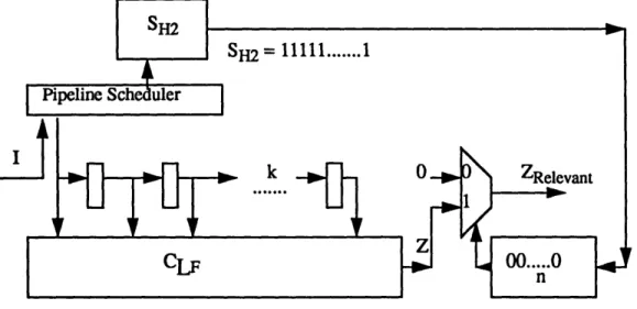
For each machine, k is the latency of each instruction. So for both machines, the first k-i outputs are irrelevant. n = k-i in PH,n.
I
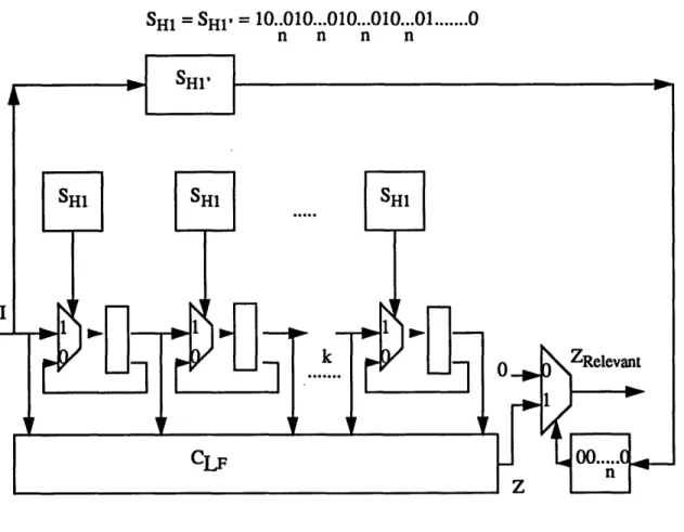
FIGURE S.Logic Transformation SG' to Unpipelined k-definite machine SG
I
FIGURE 6.Logic Transformation SF, to Pipelined k-definite machine SF
Figure 5 shows the logic transformation SG' and string function SHI to filter the relevant
outputs for the unpipelined machine SG. Figure 6 shows the logic transformation SFp and string function SH2 to filter the relevant outputs for SF (the pipelined machine). For the unpipelined machine, the inputs change every k cycles after the previous instruction has com-pleted execution, and outputs are sampled every k clock cycles. For the pipelined machine,
Microprocessors as Definite Machines for Verification
inputs change every clock cycle, and outputs are sampled every clock cycle after the first k-I cycles. Therefore by construction, comparing the outputs of the logic transformations givenpk input sequences of length k verifies the functional equivalence of the two machines.
We have different string functions SH1 and SH2 for the two machines as shown above. Fig-ure 7 shows a logic transformation SF' for the pipelined machine SF for which the string func-tions for both machines are the same, inputs can be changed and outputs can be observed at the same time for both machines.
SH1 = SH' = 10 010...010.01 .. ... 0
n
n
n
n
The string function SH1 to filter out the relevant inputs and outputs also occurs for each memory element i.e. the k registers in the pipelined machine. If a 0 is produced by SH1, the register gets its own value, else it passes its value one register forward. This is a valid logic transformation, and will not alter the state of the machine when SHi produces a 0 as the rest of the logic is purely combinational. Moreover the outputs produced at those times are not rele-vant. Again, by construction, comparing the outputs of the logic transformations given pk
input sequences of length k verifies the functional equivalence of the two machines.
4.3.4 Verification of k-definite machines with variable k
In some pipelined machines, k may vary during execution. For example, after control transfer instructions, delay slots are created, and instructions in these delay slots have to be annulled. To effectively annul an instruction, the machine may need information about instructions that may have executed ahead of it. This may increase the order of definiteness of the machine dur-ing execution.
Of the k pipeline stages in a pipelined machine, if the target of the current control transfer instruction is known in stage i, 1 < i < k, and is effective in the next cycle, all instructions issued and which are currently in stages l...(i-l) have to be annulled. If an instruction in delay slot q, I < q < (i-I) modifies the state of the machine (i.e. writes registers, modifies program counter etc., in the case of a microprocessor) in stage j, q < j k, then during stage j, instruc-tions i-q beyond stage j have to be known to annul the instruction. So now, the machine becomes max (k, j+i-q)-definite. In the worst case, we have a (2k-l)-definite machine.
Theorem 4.3.4.1 A pipelined k-definite machine, where k varies during execution can be veri-fied against an unpipelined k-definite machine, using the P-relation for synchronous machines.
Proof:
The same logic transformations as shown in Figure 5 and Figure 6 hold for verifying the two machines, except SH2 has to be modified not to include the annulled instruction outputs in the relevant values set for the pipelined machine.
Microprocessors as Definite Machines for Verification
Let the control transfer instruction have m delay slots. Then SH2 is modified as follows:
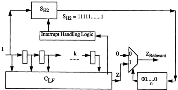
SH2 = 1 1 1 ... 1 (as shown in Figure 6)
except when an instruction is a control transfer instruction, then the next m 1 's are O's, i.e. the instructions are annulled and outputs are irrelevant. Any incorrect change in state of the machine, i.e. if any instruction is not annulled, will be detected. So the relevant outputs are fil-tered out and compared for verifying the functional equivalence of the two machines.
The length of the sequence in the unpipelined machine remains k, while in the pipelined machine, it is max(k,j+i-q). We may need sequences as long as 2k-1 where k-1 instructions are annulled. If the xh instruction is a control transfer instruction with i-I delay slots, then
1. InputUnpipelinedMachinel.... = InputPipelinedMachinel ...x,
2. InputUnpipelinedMachinex+ ... k = InputPipelinedMachinex+i ...ma (k,j+iq) and 3. outputs for InputPipelinedMachinex+1.... +i-I are not relevant.
For instructions for which outputs are relevant, the length of the sequence is k. Therefore, the number of possible instruction sequences is pk, where p is the cardinality of the instruction set. But to fill up the i-i delay slots, there would be pi-l possible instruction sequences of length i-i. Therefore the number of possible instruction sequences becomes x*pk*pil + pk,
where x is the probability of having at least one control transfer instruction in the original sequences of length k.
If z is the number of types of control transfer instructions in the instruction set, then
k k-I k-2 2 k-I
x = ( ) (1)+( )+ + ) (1) + (Z)( )
43.5 Pipelined Microprocessors with Data Hazards
A major effect of pipelining is to change the relative timing of instructions by overlapping their execution. This introduces data hazards. Data hazards occur when the order of access to operands is changed by the pipeline versus the normal order encountered by sequentially exe-cuting instructions. Consider two instructions i and j, with i occurring before j. The possible data hazards are as follows:
*Read After Write (RAW): j tries to read a source before i writes it, so j incorrectly gets the old value.
*Write After Read (WAR): j tries to write a destination before it is read by i, so i incorrectly gets the new value. This cannot happen in an in-order issue pipeline.
*Write After Write (WAW): j tries to write an operand before it is written by i. The writes end up being performed in the wrong order, leaving the value written by i rather than the value written by j in the destination. This hazard occurs in pipelines that write in more than one stage, or issue instructions out of order.
A more detailed description of data hazards and ways of eliminating them can be found in [PH90].
RAW hazards are the most common hazards and occur in most pipelined microprocessors.
We will consider only these hazards, since we are evaluating static pipelines, which issue instructions in order and in which each stage executes in one cycle, precluding WAW and WAR hazards.
The problem of RAW hazards can be solved with a simple hardware technique called
bypassing (or forwarding), which is described in [PH90]. Bypassing results in feedback from
one stage of a pipeline to one or more stages preceding that one. But this does not alter our definite machine model of microprocessors for verification purposes, as shown in the follow-ing theorem.
Microprocessors as Definite Machines for Verification
Theorem 43.5.1 Pipelined k-definite machines with bypassing can be verified against
unpipelined k-definite machines using the p-relation for synchronous machines.
Proof:
Bypass paths provide correct register values to be used by instructions during execution, and thus facilitate correct execution of the microprocessor. Without bypass paths, one would need to stall the instructions till the source operands become available.
Although bypassing results in feedback from one stage of a pipeline to a stage preceding that, the dependencies are again due to the register file values, which are observable and are allowed for verification purposes. Bypass paths just facilitate these register values to be avail-able at the time when the instructions require them as source operands.
Thus our original model of a definite machine for the pipelined microprocessor is pre-served, and the technique mentioned in Theorem 4.3.3.1 can be used to verify the two
Chapter 5
Verification of Pipelined
Microproces-sors using Symbolic Simulation
5.1 Introduction
In this chapter, the implementation of the methodology for verification of pipelined micropro-cessors is explained in detail. The methodology is incorporated into sis [SSMS92], a combi-national and sequential logic synthesis and verification system. The unpipelined specification and the pipelined implementation are specified in a high-level language BDS. These descrip-tions are then synthesized into sequential logic using BDSYN, a logic synthesis program, to
obtain slif netlists.
The user has to specify the properties of the machines, which include k to characterize them as definite machines, and d, the number of delay slots after each control transfer instruc-tion in the pipelined machine. The user also specifies simulainstruc-tion informainstruc-tion for the two machines, the use of which will be explained in the sequel.
Section 5.2 includes a discussion of verification of pipelined microprocessors with fixed k. In Section 5.3 verification of microprocessors with variable k is described. Section 5.4
Verification of Pipelined Microprocessors using Symbolic Simulation
describes some of the implementation details of observing particular variables during the sym-bolic simulation of each machine. The basic methodology of verification of simple pipelined microprocessors is extended to verify more complex machines with interrupts, traps, excep-tions and also dynamically scheduled pipelines. Section 5.5 describes verification of micropro-cessors with interrupts, traps and exceptions. Section 5.6 describes a method to verify microprocessors with dynamically scheduled pipelines. Section 5.7 gives a brief description of a method to verify superscalar pipelined microprocessors.
5.2 Pipelined Microprocessors with fixed k
In this section we consider verification of pipelined microprocessors with fixed k. The opera-tions performed by such machines would be simple ALU operaopera-tions, memory operaopera-tions with-out stalls etc. Microprocessors with variable k will be considered in Section 4.2.
The pseudocode of the algorithm for verification of the pipelined implementation with the unpipelined specification is given in Figure 8.
For each machine, the transition relation is computed for symbolic simulation. To simulate k sequences of instructions, we need to simulate the unpipelined machine for k2 cycles, and the pipelined machine for 2k-i cycles.
For each machine, the input specification functions and output filtering functions are com-puted from the simulation information provided by the user. The input function specifies what should be the instruction input in a given cycle. For now we are simulating instructions which do not alter the order of definiteness for the pipelined machine for correct execution. For the unpipelined machine, instruction i is fetched in cycle i)+l, and is an input in cycle
k(i-1)+2. At the (k(i-1)+2)th cycle, we cofactor the transition relation outputs with respect to the
inputs such that the cofactored relation corresponds to all instructions that do not alter the order of definiteness of the machine, for all i, I < i k. For the rest of the cycles, the transition relation is smoothed with respect to the inputs, since in these cycles, the inputs to the machine are irrelevant. For the pipelined machine, instruction i is fetched in cycle i, and is an input in
cycle i+l. At the (i+l)th cycle, we again cofactor the transition relation outputs as described above. Again, for the rest of the cycles, the transition relation is smoothed with respect to the inputs, since in these cycles, the inputs to the machine are irrelevant. The Boolean formula which specifies the inputs for cofactoring is provided by the user.
Verify(unpipelinedNetwork, pipelinedNetwork,simulationInfo) Compute input specification function for pipelinedNetwork;
Compute output filtering function for pipelinedNetwork; Compute transition relation for pipelinedNetwork;
Simulate the pipelinedNetwork for 2k-1 cycles;
If in a simulation cycle, the output filtering function is 1,
sam-ple the specified variables and add their formulae to the array
var-FormulaeP;
Compute input specification function for pipelinedNetwork; Compute output filtering function for pipelinedNetwork; Compute transition relation for pipelinedNetwork;
Simulate the unpipelinedNetwork for k2 cycles;
If in a simulation cycle, the output filtering function is 1,
sam-ple the specified variables and add their formulae to the array
var-FormulaeU;
for (i=1, i < K; i++) {
for (j=l, j < NUM_VARS; j++) {
verifyBddFormulae (varFormulaeU[i] [ j ], varFormulaeP [i] [ j ); if not equal then the two machines are not functionally
equivalent and exit;
FIGURE 8.Algorithm for verifying the functional equivalence of the pipelined and unpipelined microprocessors
Verification of Pipelined Microprocessors using Symbolic Simulation
The output filtering function specifies the cycle in which the variables, which are specified by the user, need to be sampled for verification. For the unpipelined machine, variables are sampled every k cycles, while for the pipelined machine, variables are sampled every cycle after the initial latency of k-I cycles.
Section 5.6 contains a discussion on variables to be observed, and verification of the BDD formulae of these variables.
5.3 Pipelined Microprocessors with variable k
We modify our methodology for verification of pipelined microprocessors described in Sec-tion 4.1 to include pipelined microprocessors with variable k. The operaSec-tions that such pipe-lined microprocessors can perform would be effective annulment of instructions in delay slots of control transfer instructions, event handling, and so on, in addition to those performed by microprocessors with fixed k.
Let d be the number of delay slots for the control transfer instruction. Let instruction Ii be the control transfer instruction, where I < i < k. The simulation strategy for the pipelined and unpipelined machines is as follows:
*Pipelined Machine:
In the pipelined machine, instruction i is the input at cycle i+1. So we simulate the machine for i cycles and compute the set of next states, as described in Section 4.1. We get the set of reachable states at each cycle and compute the total set of reachable states from the reset state.
At the (i+l)th cycle, we cofactor the transition relation outputs with respect to the inputs that specify that the current set of instructions are control transfer instructions. The Boolean formula which specifies the inputs for cofactoring is provided by the user. We then compute the set of states reachable from the current total set given the new input. In the next d cycles, which are the delay slots, we can compute the next set of reachable states by smoothing away
the inputs from the transition relation, and thus simulate all possible instructions in the delay slots. Thus we get the instruction Ii as specified and only the set of states reachable for that
instruction will be accounted for in the new total set of reachable states. The simulation for the cycles that follow is as described in Section 4.1. We simulate the machine for 2*k-I +d cycles. This will account for the delay slots in the machine and the verification algorithm will be able to check for proper annulment.
· Unpipelined Machine:
In the unpipelined machine, instruction Ii is input at cycle k(i-1)+2. So we simulate the
machine for k(i-1)+l cycles and compute the set of next states, as described in Section 4.1. We get the set of reachable states at each cycle and compute the total set of reachable states from the reset state.
At the (k(i-1)+2)th cycle, we cofactor the transition relation outputs with respect to the inputs which specify that the current set of instruction are control transfer instructions. We then compute the set of states reachable from the current total set given the new input. The simulation for the cycles that follow is as described in Section 4.1. Thus we get the instruction
Iias specified and only the set of states reachable for that instruction will be accounted for in
the new total set of reachable states. We simulate the machine for k2cycles.
Certain control transfer instructions, such as conditional branches, sample a value of a sta-tus register to decide the next instruction address. Since we are following an implicit simula-tion strategy, all possible values of the status register are considered, and the next set of states is computed using this information.
The output filtering function for the pipelined machine is modified so as to take into account the delay slots created by the control transfer instruction in the pipeline and the effect of annulment of instructions in these delay slots, i.e. sampling of the variable formulae is not done at the cycles when the instructions in the delay slots would produce outputs. Moreover,
Verification of Pipelined Microprocessors using Symbolic Simulation
more than one of 1...k can be a control transfer instruction, and accordingly the next states computations can be done and the output filtering function can be specified.
Let z be the number of control transfer instructions, and we simulate one control transfer instruction each time, then the total number of simulations required would be k*z. In this scheme, in each simulation, any one of the k instructions is one of the z control transfer instructions. Having more than one instruction as a control transfer instruction in a simulation is not necessary as the particular instruction execution is verified at all of the possible k instruction slots. This improves the efficiency of the methodology, since it does not require simulating all possible combinations of these special instructions.
5.4 Observing Specific Variables for Verification
As mentioned earlier, BDD formulae for variables are to be observed during symbolic simula-tion of each machine at specific cycles as specified by the output filtering funcsimula-tion. The vari-ables to be observed for the two machines are specified by the user. For each microprocessor the variables to be observed may include:
1. General Purpose Registers,
2. Instruction Address Register (the Program Counter PC),
3. Memory Location Contents,
4. Address to Register File and Memory for Read/Write,
5. Instruction Register,
6. ALU Operation.
Once the simulation is completed, the ROBDD formulae of all specified variables at each specified cycle for both machines are obtained. The ROBDD formulae of variables in the pipe-lined machine at a given cycle are verified with the ROBDD formulae of variables in the unpipelined machine at the corresponding cycle using combinational verification techniques as described in [Bry86]. Given two logic functions, checking their equivalence reduces to a
graph isomorphism check between their ROBDD's G1 and G2, and can be done in IG11 (= IG21) time.
5.5 Verification of Pipelined Microprocessors with Interrupts and
Exceptions
I
FIGURE 9. Logic Transformation SG' to Unpipelined k-definite machine SG with Event Handling