Autonomous Mission Scheduling for Satellite Operations
by
Birgit M. Sauer
S.B., Massachusetts Institute of Technology (1993)
Submitted to the Department of Aeronautics and Astronautics
in partial fulfillment of the requirements for the degree of
Master of Science in Aeronautics and Astronautics
at the
MASSACHUSETTS INSTITUTE OF TECHNOLOGY
September 1997
@ 1997 Birgit M. Sauer
Author...
...
Department of Aeronautics and Astronautics
August 14, 1997
Approved by ...
'V
Dr. Michael Ricard
Technical Supervisor, Draper Laboratory
Certified by...,.
... ... ....
.
Dr. Milton Adams
Lecturer, Department of Aeronautics and Astronautics
Thesis Supervisor
I
AA ccepted by ...
...
Associ te Professor Jaime Peraire
Chairman, Department Graduate Office
, 1 5 1: -N;LO3Y,
OCT151W7
Autonomous Mission Scheduling for Satellite Operations
byBirgit M. Sauer
Submitted to the Department of Aeronautics and Astronautics on August 14, 1997, in partial fulfillment of the
requirements for the degree of
Master of Science in Aeronautics and Astronautics
Abstract
When reducing the operations costs of a satellite program, planning and scheduling are a prime areas for consideration. In particular, scheduling satellite activities is repetitive, time-consuming, and non-trivial. Automating the planning and scheduling tasks can reduce operator staffing requirements, and increase the utility of the satellite. Additionally, since the main cost of an automated scheduler is its development, being able to use the scheduler for different satellite programs would lead to great cost savings. Since there is such variety in satellite programs, no realistic scheduler can be easily reused for them all. Automated schedulers can, however, be developed for "classes" of satellites that share the same fun-damental characteristics. This thesis describes a scheduler for three different classes: spin stabilized science satellites; 3-axis stabilized, earth observing science satellites; and constel-lations of 3-axis stabilized, earth observing science satellites. Each scheduler uses a linear programming model of its mission, optimizing the value gained from the use of the instru-ments given a set of constraints. As a proof of concept, each scheduler is demonstrated in a case study. Finally, consideration of dynamic rescheduling in response to system failures is provided in an additional set of case studies.
Thesis Supervisor: Dr. Milton Adams
Acknowledgments
There are many people to whom I owe a great deal of thanks: to Michael Ricard for answering silly questions without laughing; to Stephan Kolitz for his enduring sarcasm in a world that takes itself too seriously; to Milton Adams for his sane views on the treatment of graduate students; to Jim Kuchar for taking the time to cover the thesis in red ink; to Eileen Dorschner for prying obscure articles out of their dusty resting places; to Draper Laboratory for the opportunity to do this research; and to all of you who made me laugh. and remember that there is more to life than the thesis due date. Thank you!
This thesis was prepared at The Charles Stark Draper Laboratory, Inc., under IR&D 710 and Contract NAS5-32007.
Publication of this thesis does not constitute approval by Draper or the sponsoring agency of the findings or conclusions herein. It is published for the exchange and stimulation of ideas.
Permission is hereby granted by the author to the Massachusetts Institute of Technology to reproduce any or all of this thesis.
Birgit Sauer August 14, 1997
Contents
1 Automated Scheduling 12
1.1 Mission Planning and Scheduling .... .. ... . . . . .. . . . 13
1.2 Problem Statement ... ... 15 1.3 Literature Review ... ... ... 16 1.3.1 Scheduling Theory ... ... .. 17 1.3.2 Satellite Scheduling ... ... ... ... 19 1.3.3 Schedule Versatility ... ... ... ... 23 1.3.4 Standardization ... ... ... ... 25 1.4 Thesis Structure ... ... ... 26
2 The Satellite Scheduling Problem 27 2.1 Problem Description ... . . ... ... .... ... .. 27
2.1.1 Inputs . . . . 27
2.1.2 D ecisions . . . .. . 29
2.1.3 Output ... 30
2.1.4 An Exam ple ... ... ... ... .. ... ... 30
2.2 Integer Programming Approach ... ... 31
2.2.1 Decision Variables . . . . ... . .. . . . . 32
2.2.2 Objective Function . ... . .. ... 33
2.2.4 The Solution ...
3 Scheduling Spin Stabilized Science Satellites 37
3.1 Modeling Assumptions ... 37
3.2 Class Description ... ... .. ... .. 38
3.3 Mathematical Programming Formulation . ... . . . 39
3.3.1 Basic Approach (Formulation I) . ... . . 39
3.3.2 Split Approach (Formulation II) . ... . . . 46
3.3.3 Instrument Only Approach (Formulation III) . ... 49
3.4 Case Study: TERRIERS ... ... 51
3.4.1 The Model ... ... ... ... .. ... .. 53
3.4.2 Results ... ... ... 56
4 Scheduling 3-Axis Stabilized Science Satellites 62 4.1 Class Description ... ... 62
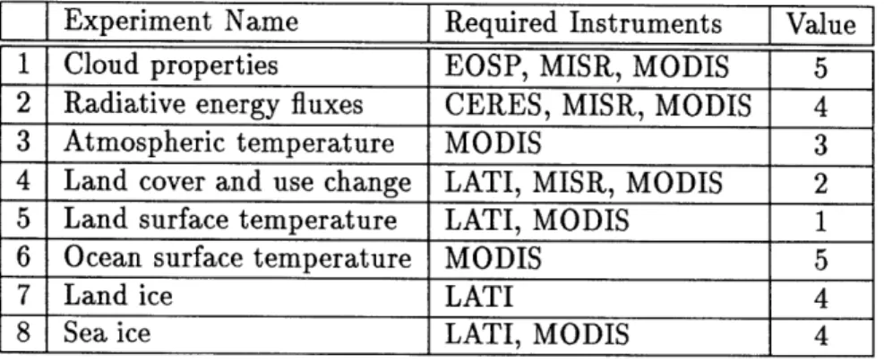
4.1.1 Instrum ents ... ... . .. 63
4.1.2 Experiments ... ... 64
4.2 Mathematical Programming Formulation . ... 66
4.3 Case Study: EOS AM-2 . ... . . . . 69
4.3.1 The Model ... . ... ... .. ... ... .71
4.3.2 Results . . . 74
5 Scheduling Clustellations of Science Satellites 76 5.1 Class Description ... .... ... 77
5.2 Mathematical Programming Formulation . ... 78
5.2.1 Grid Approach (Formulation I) ... .. . . . ... 79
5.2.2 Overlap Approach (Formulation II) . ... 82
5.3 Effective Experiment FOV ... 85
5.3.2 5.3.3 5.4 Case 5.4.1 5.4.2 5.4.3
Two Instrument Case ...
Effect of Separation Angle on Effective Experiment Study: EOS AM-2 ...
Case I: 5 Satellites ... Case II: 3 Satellites ...
Case III: 5 Satellites, Different Experiment Set . . FOV
6 Uses for an Automated Scheduler
6.1 Mission Scheduling ... 6.2 Rescheduling ... 6.3 Failure Analysis ...
6.4 Sensitivity Analysis and Design Trade-offs 6.5 The Ideal Level of Automation . . . . 6.5.1 Levels of Automation . . . . 6.5.2 Comparing Levels of Automation .
7 Conclusions and Future Work
7.1 Overview . . . . 7.2 Capabilities . . . . 7.3 Limitations . . . . 7.4 Future Work . . . . 7.5 Conclusion . . . . Bibliography
A Effective Experiment FOV for Three or More Instruments
B Tilted FOV Calculation
. . . 87 . . . . 90 .. . . 92 ... . 94 . . . . 97 ... . 101 104 104 106 107 109 113 114 114 119 119 120 121 122 123 125 129 134
List of Figures
2-1 Growth of a combinatorial problem. . ... . . . . 29 2-2 An optimal solution to the example problem. . ... 32
3-1 A complete constraint matrix comprised of four decoupled sub-blocks. . . . 44
3-2 A complete constraint matrix for a time line of four time steps that are mostly
decoupled .. . . . .. . . . 45 3-3 The formulation for one night time step of spectral mode. . ... 57 3-4 Illustrative segment of the resultant week long schedule. . ... 59
3-5 Illustrative segment of the default week long schedule assuming a 50% duty cycle on all the instruments ... 60
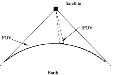
4-1 Illustration of a satellite's field of view (FOV) and instantaneous field of view (IFOV ). . . . . . . . .. . 64 4-2 The FOV of a nadir pointing instrument. ... ... 65 4-3 The experiment FOV is the intersection of the area all of the instrument FOVs. 66 4-4 Launch timetable for the major EOS satellites. . ... 70 4-5 The schedule for one orbit of the EOS AM-2 sample problem. . ... 75
5-1 Illustration of a Walker Delta constellation viewed from the north pole. . . 77 5-2 Three example cluster configurations. . ... .. 78 5-3 The effective experiment FOV for an experiment requiring three different
instruments is the intersection of the three different instrument FOVs. . . . 82 5-4 The time integrated instrument (or experiment) FOV is a swath across the
5-5 The actual FOV for an instrument and its linear approximation. ... . 87 5-6 While each instrument FOV can be approximated as a flat surface, care must
be taken to preserve the actual center to center separation distance .... 88 5-7 Illustration of the coordinate system used to calculate the effective
experi-ment FOV. 89
ment . . . .. . .. . . . . ... ... ... .... .... .... ... 89
5-8 Effective experiment FOV width and area as functions of separation angle. 91 5-9 An illustration of various separation angles. ... . . . . . . . . . . 92 5-10 Effective experiment FOV width as a function of separation angle for an
experiment requiring only the three tilted MODISs ... 99 5-11 Schedule for one orbit of Case II. ... .... 100
5-12 Schedule for one orbit of the nominal case using the new experiments and resource amounts from Case III. ... . ... .. 102 5-13 Schedule for one orbit of Case III with a separation angle of 50. ... 103 5-14 Schedule for one orbit of Case III with a separation angle of 110. . ... 103 6-1 Schedule value as a function of available power as generated by the scheduler
(both given as a percentage of nominal) . . . 110 6-2 Schedule value as a function of available power as generated by theory (both
given as a percentage of nominal) . . . . . . 112 6-3 A presumed curve of life cycle cost versus the level of automation. ... 113 A-1 The top and bottom bounding points of the effective experiment FOV. . . . 130 A-2 Zero effective experiment FOV ... 130 A-3 The next bounding point is the point closest to the old point in a clockwise
direction ... ... ... .. ... ... 131 A-4 The finished algorithm produces a list of bounding points and ellipses. . .. . 131 A-5 If no intersection points are found, the effective experiment FOV is the FOV
of the center instrument ... ... 132 A-6 The ellipse that connects the two boundary points is centered between the
two points... .. .... ... 132 A-7 The ellipse that connects the two boundary points is centered either above
B-1 The FOV of a tilted instrument is longer than that of a nadir pointing
in-strument. ... ... 134
List of Tables
2.1 Relative values of data for one time step from each instrument in the example
(science points) ... 30
2.2 Resource usages of each instrument in each mode in the example... 31
3.1 Relative values (in science points) of each instrument in the sample TERRIERS problem . . . .. . . . . 55 3.2 The total available amount of each resource and the usages for each
instru-ment for each resource in the TERRIERS sample problem... . . 55 3.3 Statistics on scheduling the TERRIERS sample problem for varying durations,
using a 15 minute time step ... 57 3.4 Statistics on scheduling the TERRIERS sample problem for varying durations,
using a 5 minute time step. ... 58
4.1 Experiment topics, instrument requirements, and values (in units of science
points) ... . ... .. 72
4.2 Resource usage values for each instrument. . ... 73 4.3 Statistics on scheduling the EOS AM-2 sample problem. . ... 74
5.1 Down range (DR) and cross track (CT) dimensions for each of the instrument F O V s . . . .. . . . .. . . 93 5.2 Resource usages for each instrument. . ... ... 94 5.3 Available satellite resource amounts and their renewal rates for the nominal
case and Case I ... ... .. 95
5.4 The experiment and modulator values for the nominal case, and Case I with a 50 and 11' separation angle (Me based on FOV width). . ... 96 5.5 Science value of the nominal and each Case I schedule given in science points. 96
5.6 The experiment and modulator values for the nominal case, and Case I with a 50 and 110 separation angle (Me based on FOV area) . . . . . . 97 5.7 Science value of the nominal and each Case I schedule in science points (Me
based on FOV area) ... ... 97 5.8 The instrument FOV dimensions for Case II. ... 98 5.9 The experiment definitions, values and modulators for the nominal case, and
Case II with a 50 and 120 separation angle. . ... 100 5.10 Science value of each schedule (in science points) in Case II ... 100 5.11 The experiment definitions, values, and modulators for for the nominal case,
and Case III with a 50 and 110 separation angle. . ... 101 5.12 Science value of each schedule (in science points) in Case III. . ... 102
6.1 Science generated by the old optimal schedule and the new optimal schedule due to various failures (given as a percent of nominal) . . . . . . 108 6.2 Amount of science generated, given that various failures have occurred (as a
Chapter 1
Automated Scheduling
The need to reduce the cost of developing, building, and operating a satellite program has been steadily intensifying. Not only are the systems themselves becoming more complicated and therefore more expensive, but the available funding is also being cut back. The insti-tutions that fund pure science missions, like NASA, are undergoing budget cutbacks and are driven to less expensive programs (hence the "faster, better, cheaper" paradigm). And commercial satellites have always been driven by the need to make a profit in the face of competition from both space- and ground-based systems.
As a result, satellite programs are becoming more streamlined and efficient. Most of the work to date has been in the portions of the program that incur the large, non-recurring costs: design, manufacture, and launch of the satellite. However, the costs associated with the recurring operations, such as scheduling, data archiving, and orbit maintenance, are a large part of the overall system cost and need to be examined more closely.
One of the important operations tasks is the planning and scheduling the satellite activities once the satellite is in orbit. Without a schedule, the mission cannot proceed. Moreover, since the schedule determines how efficiently the available resources are used, the quality of the schedule, affects the overall mission value. In addition, scheduling is not a trivial task. The sheer size of the scheduling problem makes it difficult to develop a good schedule, much less the best schedule.
Acknowledging this, many of the larger programs have developed and implemented auto-mated schedulers [22, 27, 30, 37]. However, those developments have been expensive and generally not reusable since the finished scheduler does not adapt easily to other programs. Smaller programs on stricter budgets do not have the resources to develop such aids. It is, however, possible to develop a scheduler that generates optimal or near-optimal sched-ules that is easily adaptable to other satellites with the same type of mission. This thesis develops a proof of concept scheduler for several different types of satellite programs.
1.1
Mission Planning and Scheduling
This thesis defines a "schedule" as a time line of operations to be executed, a "feasible schedule" as a schedule that does not violate any of the constraints on the system, and an "optimal schedule" as a feasible schedule that, if executed, would generate the highest possible mission value. "Planning" refers to the entire process of creating and executing a schedule. "Scheduling" refers specifically to that part of the planning process focused on creating the schedule. The rest of this section describes the planning process in detail so this distinction will be more clear.
Planning a satellite mission involves the following tasks:
* Gathering a list of potential operations * Deciding which operations will be executed
* Ordering the operations on a time line (scheduling)
* Verifying the schedule as feasible
* Uplinking the schedule to the satellite
* Executing the schedule
* Processing and distributing the results
For example, the "operations" to be executed for a scientific imaging mission are collecting the images or sets of images of the desired areas (referred to here as "experiments"). The
list of all the proposed experiments is compiled from all the participating scientists. Then, assuming that not all the requested experiments can be executed due to resource limitations, some subset of them is chosen. Generally speaking, this is decided by means of a peer review. For each experiment that is chosen, all the requirements and constraints are characterized in such a manner that they are intelligible to the scheduler. The scheduler then orders all these experiments on a time line (schedules them). Before the schedule is uplinked to the satellite, however, it is checked to insure all the constraints are honored. Finally, once the schedule has been executed, the resulting data are downlinked and archived for future use.
Example of a Complex Planning System
One of the most intricate planning systems is the planning system for the Hubble Space Telescope [25, 30, 44, 54, 70]. While the determination of which experiments to include in a year's observations is left to a human review panel, the rest of the system is automated. The process works as follows. A scientist submits a proposal for an experiment in two phases. Phase I is an overview of the experiment and is submitted to the review board. The review board determines which of the tens of thousands of proposals will be accepted for the year based on value judgments such as chance of success, relevancy, and preparedness. Note that these value judgments are the reasons why this phase is not automated.
If the proposal is accepted, the scientist completes Phase II of the proposal in which he details all the requirements of the experiments. From this point on, the planning process is automated, although the human operator can override the computer at any point. The proposal is submitted in a standard form set by the Remote Proposal Submission System (RPSS), which can be accessed on the world wide web. Because the request is now in a standard format, it can be converted into a "scheduling unit" automatically. A program called Transformation (TRANS) accomplishes this, while another program, the Proposal Entry Processor (PEP), places the unit on the schedule as though it were the only unit to be scheduled that year. This serves to highlight the preferential times for each experiment and times that are in demand by many experiments. Another "meta-level" scheduler called the Criterion Autoscheduler for Long Range Planning (CASL) was added to the system to help schedule experiments that cannot be written in the pre-defined manner and to help make schedule changes once all the experiments are input into the system. Then the long
term scheduler, Science Planning Interactive Knowledge Environment (SPIKE), generates a schedule with each experiment assigned to a specific week of that year. Since the review panel approves roughly 30% more experiments than can be accommodated in a year, SPIKE must decide which requests will be honored and insure that the final schedule is feasible. The Science Planning and Scheduling System (SPSS) sorts out the schedule for each week. Once the images have been taken, they are sent to the Space Telescope Data Archive and Distribution Service (ST-DADS) for processing and storage. Data can be retrieved from the archive over the Internet using a software program called StarView.
1.2
Problem Statement
The basic satellite scheduling problem can be stated as follows: Develop a schedule that, if executed, would allow the satellite to produce the maximum amount of value while satisfying all of the physical and operator imposed constraints on the mission, the satellite, and the instruments.
These constraints come in many forms. Some are due to instrument limitations (for ex-ample, an instrument might only be able to operate for a given length of time before it overheats). Others are due to resource limitations (for example, the amount of power on-board is generally limited and must be shared by all the instruments). Yet others are due to satellite limitations (for example, the satellite is not radiation hardened enough to pass through the South Atlantic Anomaly without shutting down). There are also schedule con-straints such as "the experiment needs to run at dawn any day in the month of May," or "whenever the first experiment is run, the next three need to be run at exactly 24 hour intervals after it." Understanding all the constraints is a feat in and of itself, much less generating an optimal schedule that honors all of them. A scheduling method that does not require a human scheduler to schedule every event individually is necessary.
The ultimate scheduler would be an automated scheduler that could be easily modified for any possible satellite. However, satellites come in many shapes and sizes with widely different missions. A completely generic scheduler is in danger of quickly becoming too large to be easily adapted to different missions. It is, however, possible to categorize satellites
and create a scheduler that is generic with respect to a class of satellites. A class is defined by the characteristics inherent in the satellite mission and design. A satellite with an earth-orbiting mission will have very different requirements than one with a sun-earth-orbiting mission, as will science, military, and communications satellites. The goal is to group satellites that share common mission driving features. Developing a generic scheduler for one class is therefore much easier than for all possible satellite configurations.
This thesis describes a proof of concept scheduler for each of three satellite classes. Note that only scheduling is addressed, not any of the other tasks involved in planning. Moreover, only payload activities are discussed. Any satellite has two types of activities that need to be scheduled: payload activities, such as when to turn on the instruments; and bus activities, such as when to fire the station keeping thrusters. While there is no theoretical reason the bus activities cannot be scheduled with the same scheduler, they are not included here in the interest of keeping the schedulers small and easy to understand.
1.3
Literature Review
The Hubble Space Telescope is an example of an almost completely automated satellite program that uses entirely custom built software. This software demanded extensive de-velopment, but needs relatively little manpower to operate. Naturally, the entire planning process could also be accomplished manually with a large stack of paper. This requires al-most no development, but the manpower involved in running the "scheduler" is prohibitive. Most satellite programs opt for a middle ground.
Some tasks lend themselves to automation. Data storage, for instance, is much more com-pact and accessible on a computer than in hardcopy. Commercial off-the-shelf data base programs can be customized for those satellite programs that do not have the time or money to develop a custom built program. Simple Gantt chart programs, like Microsoft Project [71], are also available commercially and aid the scheduling process by graphically showing the schedule as it is built.
Other pieces of software, like Draper Laboratory's Timeliner [7], are custom built for one satellite program but were designed to be adaptable (Timeliner was originally developed
for the international space station). It is a computer language that helps streamline the planning process by having built in constructs such as "before" and "after." This makes it easier to submit requests in the format required by the scheduler. It also makes it easier to create constraint checking programs that test the feasibility of a finished schedule.
Schedulers themselves, however, are generally not adaptable. Since the scheduling problem. is complicated, many schedulers make assumptions based on the particular satellite mission that do not transfer well to other missions. The underlying theory, however, is not mission dependent.
1.3.1 Scheduling Theory
Scheduling events is by no means limited to satellite payloads. As scheduling theory is much older than the satellite industry, the formal, theoretical work has been done with regard to other systems, mainly manufacturing systems. While there are many different problems associated with a manufacturing plant, the main category of problems is "job shop scheduling." The basic job shop model is one wherein there is a set of jobs to be completed, each consisting of a certain number of individual operations. Each operation is performed on one of a set of machines. Furthermore, there are constraints on the system. One such set of constraints might be that the machine on which each operation is to be performed and the order of the operations within a job are specified a priori. The goal is to find the schedule that minimizes the time it takes to complete all the jobs while still satisfying the constraints [41].
The problem as stated is NP-hard [20]. Generally speaking, such problems are solved to near-optimality using heuristics. There are also many variations on the basic problem, some of which are also NP-hard, others of which are solvable in polynomial time. There might be several machines of the same type, so each operation is not constrained to only one machine. The order of the operations might not be set a priori. There might be resource constraints, such as operator manpower or storage space for the finished goods, on the system. Or the particular problem might have a different objective function, such as minimizing the idle time of the machines.
The satellite scheduling problem can be cast as a job shop problem. For a scientific imaging mission there are some number of experiments (jobs) to be executed. Each experiment consists of a set of images (operations) that must be collected by one of a set of instruments
(machines).
While not drastically different, the set of constraints on a typical satellite problem varies* from that on the basic job shop problem outlined above. The images must be collected by a certain instrument, but the order of the images is not necessarily important. Instead, each image has a range of absolute times when it can be taken (e.g., only at night, only when the supernova is in view, etc.). There are also resource constraints on both the satellite and the instruments. The entire satellite has limited power and data downlink capacity, while each instrument has limited cryogenic coolant. Note that different satellite missions will also have different constraints.
Unlike the job shop problem, the completion time in the satellite problem is fixed. Instead, the objective is to maximize the value of all the experiment data collected in that time. Alternately, the objective may be to minimize the unused resources.
The satellite scheduling problem also incorporates aspects of two other optimization prob-lems: the knapsack problem and the traveling salesman problem. The knapsack problem is the problem of packing a knapsack of finite volume with an assortment of objects, each with a value and a volume. The problem is to get the most valuable pack without exceeding the volume limits. While this problem is NP-complete in theory, in practice it can usually be solved in pseudo-polynomial time [35]. Similarly in the satellite scheduling problem, each observation has a value and uses a certain amount of resources. The satellite as a whole has a limit on the total amount of resources available. However, the satellite problem also has time constraints that cannot be modeled by an equivalent knapsack problem.
Given a set of cities, the traveling salesman problem finds the best route for the salesman so that he sees all of them only once. This problem is NP-complete [35] and generally solved by heuristics. A satellite also "travels" by slewing its instruments so that they can point at each "city." The problem is, the traveling salesman problem assumes the set of cities is known, which is not necessarily true for the satellite problem, and it has no way of handling resource constraints.
The formulations described in the following chapters are loosely based on the job shop scheduling problem, both because that is the closest to the satellite scheduling problem and because it is the easier one to modify.
1.3.2 Satellite Scheduling
The following is an overview of the scheduling practices in use on various satellites. Each satellite program has its own planning system and no attempt was made to try to document them all. Instead, the goal is to give the reader a sense of the types of schedulers in use and some familiarity with the more common systems.
Manual Scheduling
Some of the first schedulers were little more than aids to the human scheduler. A method that uses rolls of butcher block paper on a conference table and a set of pencils, although not the most efficient in terms of manpower was used for a long time [18]. Computerized versions of the butcher block paper were also developed [65, 71, 72]. Colorizing schedules make them easier to understand at a glance. The amount of each resource used can also be calculated automatically instead of laboriously with a calculator. And the computer can also check all the constraints and flag those that are violated. Note that while this acts as a very convenient aid to the human scheduler, the actual scheduling is still done manually. The human scheduler places every experiment on the time line individually.
Envelope Scheduling
One of the simplest and least time consuming scheduling methods employed for a system with several users is the "envelope method." Instead of defining the schedule down to the last detail, mission command divides the satellite resources into blocks or "envelopes" that each user is allowed to use as he sees fit for the entire working lifetime of the satellite. Each user is then responsible for his own schedule. As long as each user does not command more resources than alloted to him and does not violate any system constraints, the final schedule is nearly feasible. Any conflicts remaining are worked out by the mission command. In this
manner, mission command does not need to know the details involved in scheduling each experiment, and does not need to put a large effort into scheduling a complicated system
[51].
For satellites that can only support one user at a time, the envelope method is not very useful. For instance, any satellite with several instruments that share the same optics falls' in this category. A related, scheduling method which is more useful in these cases is called
"coarse graining." Each experiment is allocated a block of time, rather than blocks of resources. For that time, the experiment has full use of the satellite's resources. Coarse graining is not quite as easy a scheduling method as the envelope method since mission command needs to know enough about each experiment to be able to schedule the blocks of time. However, mission command does not need to concern itself with fine details, and the scheduling problem it is solving is still considerably smaller than that for the entire system. This scheduling method has been used quite successfully on the International Ultraviolet Explorer (IUE) for over 15 years [23, 29].
Many satellites have experiments that can be run simultaneously but that do not need a constant amount of each resource all day long. They generally run during only part of the day, week or year. Both the envelope and the coarse graining methods are very inefficient for these systems. In these cases, a variation of these methods can be used. Resource envelopes are allocated to experiments but the envelope sizes vary with time. Such a system was tested in the Earth Observing System (EOS) testbed and was a success. Moreover, it was found that it worked best when the users themselves requested certain amounts of resources at certain times. When conflicts arose, the users were informed and left to sort the schedule out for themselves. EOS will use this system for all of its satellites [39].
Note that the envelope method does not produce an optimal schedule. An optimal schedule produces the highest value possible by using the available resources in the most efficient manner. In the envelope method, any resources not used in any allotment are lost. Mission command can make adjustments and improve the schedule if it knows one user needs 20 more watts of power and a second user has them to spare, but on the whole, depending on such swaps is not practical. What is kept to a minimum with the envelope method is the effort mission command must expend on scheduling.
Heuristic Scheduling
Schedules that use resources in a more optimal manner assign an experiment only the resources required for only the time needed, allowing for a much more efficient schedule.
The problem is that there are now many more possible start times, and it is much easier to accidently over subscribe resources. In other words, the problem is much more complex and correspondingly harder to solve.
Given a partial schedule and the next experiment to schedule, determining all the possible times for which that experiment could be scheduled is a painstaking and time consuming job that can be accomplished by a computer. One scheduling method is to let the human scheduler decide which experiment to schedule next, let the computer find all the possible time slots for that expefiment and then let the human decide which time slot to actually schedule the experiment in. The Advanced Communication Technology Satellite (ACTS)
[37] uses this type of system.
In order to choose which experiment to schedule next and to decide which time slot to schedule it in, the operator is, consciously or unconsciously, employing a set of prioritizing rules. The most valuable schedule is chosen, where "value" is determined by these rules. When these rules are written down they are referred to as "heuristics."
The schedule can be determined by a computer if these heuristics are pre-defined. Exper-iments are placed on the time line in an order and place determined by the heuristic(s), insuring that the schedule does not violate any of the constraints. Note that very often sev-eral heuristics will be used in a hierarchical fashion. Some of the more common heuristics used are: scheduling the most valuable experiments first ("greedy heuristic"); scheduling the most crowded time slot first; scheduling the longest experiments first; and scheduling everything as early as possible. Maestro is a heuristic based scheduler for the Japanese Experiment Module (JEM) on the Space Station [27]. The Clementine mission also used a heuristic based scheduler for their Autonomous Operations Scheduling (AOS) experiment [43]. In the latter case, the scheduler is used to generate both the payload activity and the satellite bus activity schedules.
the constraints. While the resultant schedule might not be feasible, this initial schedule can be determined quite fast. Then a repair algorithm or heuristic is used to create a feasible schedule from the initial schedule. The long term scheduler for the Hubble Space Telescope, SPIKE, uses this methodology [25]. The initial schedule is created using a min-conflict heuristic that schedules the most constrained experiments first. Repair heuristics based on experiment priority and number of conflicts are used to improve the schedule. This repair phase is ended when some pre-established level of effort has been reached. Then the schedule is "de-conflicted". The least valuable experiments are removed until the schedule becomes feasible. Any gaps in the schedule after this de-conflicting are filled by a "best-first" heuristic.
The Space Based Visible (SBV) sensor onboard the Midcourse Space Experiment (MSX) satellite uses a scheduler called SBV Processing, Operations and Control Center (SPOCC). A list of targets to be used is supplied by the Ballistic Missile Defense Organization (BMDO). Then each target is assigned a value determined by its priority and availability (the targets are not visible all the time). The schedule is created in real time by scheduling the sensor to look at the current most valuable target [45, 49].
Optimized Scheduling
The schedules generated with heuristics, while feasible and better than most, are not typi-cally optimal. Because of the difficult nature of the problem, there are very few schedulers that produce optimal schedules. Some schedulers, however, come close. The European Resource Satellites (ERS-1 and ERS-2) use a scheduler called PlanErs. It creates an initial feasible schedule using heuristics. Then experiments are removed and added according to another heuristic in an attempt to improve the schedule. Each schedule is saved in memory so that schedules are not duplicated. If the scheduler is allowed to run for long enough, the result will be the optimal schedule. Note that generally, the scheduler is stopped after some pre-defined amount of time and the current best schedule used even though it is not the optimal one [22].
Maestro II uses a combination of optimization techniques and heuristics to solve for the best schedule. The problem is written as an integer program, maximizing the overall resource
usage. However, in solving the problem, branching heuristics based on the value of each experiment are used to make the search space smaller [27].
The Advanced X-Ray Astrophysics Facility - Imaging (AXAF-I) determines the list of targets for the day using heuristics based on some science goal (for instance, maximize time an science targets or minimize thruster fuel consumption). Then the schedule is determined by an optimization algorithm. The final schedule is optimal with respect to that day's
target list although not necessarily with respect to the mission's target list [32].
One of the more unique scheduling algorithms models the satellite as a robot arm over a 2-D field. As the arm makes straight passes over the field, it needs to pick up objects of varying value. Both the value and the position of each object is known a priori. In this manner, the motion of a satellite tracking spots of interest on the ground is modeled. The time it takes the satellite to turn its optics to focus on a target is modeled by the time it takes to move the robot arm from one object to another. The schedule is generated using genetic algorithms: a "population" of possible schedules is set up and mutations of those schedules result in other schedules. Good schedules are returned to the gene pool while bad schedules are removed [1].
1.3.3 Schedule Versatility
Robustness
In developing schedules, there is a trade off between optimality and robustness. Scheduling experiments on a time line in an efficient manner is one challenge. However, that schedule must be carried out by a very complex system prone to unexpected events. Experiments might take longer or use more resources than expected, one experiment might suddenly become infeasible due to a malfunction or atmospheric events, or new experiments might be added at the last minute. If this happens when the satellite is following a very efficient schedule whose events are tightly packed in time and resources, the flow of the schedule is interrupted. Perhaps the current event will not be completed. Or perhaps an event will have to be dropped altogether. Or perhaps some future event will have to be curtailed or dropped. When this happens, the schedule is no longer optimal and is said to be "broken."
Less optimal schedules, on the other hand, tend to be more robust because there is slack in the system. Schedules created with the envelope method tend to have unused time and resources built into them. This makes them less optimal, but less likely to break since any small deviation from the expected events can be absorbed into the schedule. Note that the schedule can be broken by a deviation that requires more time and resources than are available.
Dynamic schedulers, like SPOCC, create schedules in real time. Whenever one experiment finishes, the next is started, so it is almost impossible to break the schedule. They do not, however, produce schedules that are optimal over time.
Systems such as PlanErs and those based on genetic algorithms that create schedules by continuously improving the current schedule by adding and subtracting different experi-ments also tend to be more robust. If an experiment is added or changed, it can be added to the pool of untried experiments and the scheduler can be allowed to continue without having to be restarted.
Rescheduling
Once a schedule breaks for any reason, a new schedule has to be generated. For some of these schedulers, like SPIKE, the entire schedule has to be redone. Others have ways to avoid regenerating the entire schedule. For the most part, these techniques capitalize on the fact that a schedule usually breaks in one place for one reason. The entire schedule doesn't need to be regenerated, just one portion of it.
Some schedulers use the broken schedule as an initial schedule and use their scheduling heuristics to create a new, feasible schedule. Others use a local repair approach. They swap experiments in and out of the broken section of the schedule according to some pre-defined set of rules until the schedule is once again feasible. Other schedulers recognize the fact that when a schedule breaks, it is because a small set of constraints have been violated. Instead of repairing the schedule by rearranging the experiments that come right before and after the broken section, they rearrange the experiments that are important to the broken constraints [47].
One scheduler used to create schedules for automated ground-based telescopes uses "pre-dictive error management" to aid in the rescheduling process. This scheduler uses the fact that schedules often break in predictable places. During the times when the telescope is not being used, the scheduler calculates the places and manners in which the schedule is most likely to break. Then an alternate schedule is created for that contingency. If that particular break occurs, the schedule is activated. Naturally, not every contingency can be accounted for, nor is this a good scheduler if the system has no spare CPU time [46].
Adaptation
While most satellite systems have schedulers that are custom designed, there has been some effort made to adapt schedulers from one satellite mission to another. The most notable is the long term Hubble scheduler, SPIKE. It has been used for several other observatory satellites such as the Extreme Ultra-Violet Explorer (EUVE) [66], X-Ray Timing Explorer XTE [59], and the RSntgen Satellite (ROSAT) [33]. While all three efforts have commented that SPIKE's GUI is extremely well developed, only the ROSAT effort reports any resound-ing success. The other two efforts report that while SPIKE is well designed, it makes many assumptions about the system that are just not true for their systems. On the whole, the conclusion reached is that it might have been easier to develop new schedulers.
The AXAF-I scheduler is also based on SPIKE, but only in the sense that it reuses the code from the scheduling engine [32]. The new scheduler has a very different methodology and
was reported a success.
1.3.4
Standardization
In line with this effort to reuse schedulers, there is also some effort in the satellite industry to standardize the interfaces of the system so that not every satellite is custom designed. SuperMOCA is a group of industry and government officials who are interested in stan-dardizing uplink and downlink formats [2, 56]. There is also some effort being put into standardizing the human-computer interfaces [26, 38]. While the industry in general is very aware that a standard GUI would eliminate confusion and retraining from one satellite
program to the next, no consensus has been reached about that standard.
Satellite buses themselves are also slowly being standardized. Various satellite manufactur-ers are beginning to develop standard buses that can be used for any mission [4, 48]. Like a launch vehicle, each bus will have limited power, communications, and volume, and have a preset price. Each mission will determine the best bus for its payload.
All these modifications are in the interest of bringing down the development and operations costs for satellite systems. Better schedules make the satellite more efficient for the same cost, and standardizing the system eliminates some of the start up time and cost for the same efficiency.
1.4
Thesis Structure
While this chapter has been an overview of existing satellite planning and scheduling sys-tems, the next chapter describes the basic satellite scheduling problem in detail. It also gives a brief introduction to the mathematical programming theory that is used to solve the scheduling problem.
Chapters 3, 4, and 5 present the formulations for the schedulers for each of the three classes of satellites: spin stabilized science satellites; 3-axis stabilized, earth observing science satel-lites; and constellations of the latter. The capabilities of each scheduler are demonstrated in a case study. Chapter 6 describes the utility of an automated scheduler and Chapter 7 details some conclusions and future work.
Chapter 2
The Satellite Scheduling Problem
This chapter is designed to familiarize the reader with the satellite scheduling problem. The problem goal and constraints are described here, along some background on the solution
theory.
2.1
Problem Description
For a non-pointing satellite, the satellite scheduling problem is to determine which instru-ments should be on at each instant in time in order to produce the maximum value without violating any of the specified constraints. To be able to do so, information about the satellite, the instruments onboard, and the mission must be detailed.
2.1.1 Inputs
The inputs fall into three distinct categories, each discussed in more detail below: * Time line information
* Data taking mode information * Satellite and instrument information
Time Line Information The scheduling horizon (i.e., the length of time for which the
schedule is active) must be specified. Typically this is a day or a week. In contrast, a long term scheduler may be expected to produce a schedule for a year or longer. In the approach taken here, the scheduler discretizes the scheduling horizon into time steps of equal length. The length of a time step is also an input. In addition, the start date of the scheduling horizon and the parameters of the satellite's orbit must be specified.
Each time step is characterized by the operating condition of the satellite at that time. Typ-ical time step types include day (when the satellite is in sunlight), night (when the satellite is in eclipse), and sleep (when the satellite is shut down for safety or other operational reasons). There are many other characterizations of the operating conditions that may be important as well (for example, atmospheric conditions, such as auroras, or geometric conditions, such as having a clear line of sight to a ground station). Conditions of interest must be predetermined by mission control. Note, however, that all of these conditions are functions only of the date and the satellite's orbit, and can be determined well in advance of the actual event. Therefore, the time line, which is a list of each time step and its type, can be generated for input either manually or by a computerized orbital propagator.
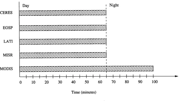
Data Taking Mode Information Instruments can operate in different data taking
modes. For instance, a science satellite might have one mode to measure over a wide spectral range but only in specific geographic areas and another mode to measure over a wide geographic range but only over select spectra. The desired percentage of time to be spent in each mode is an input and the scheduler will determine the active mode for each time step. If no instruments are on, the satellite is considered to be in sleep mode.
Note that "sleep" is used in two different contexts here: as a data taking mode and as a time step type. In both it means that the satellite is shut down, and all instruments are off. The difference is whether the condition is commanded by mission command or scheduled by the scheduler. For example, a sleep time step may be commanded as input if the physical conditions of the orbit require it (perhaps as the satellite passes through the South Atlantic Anomaly to avoid operating in a high radiation environment). Thus, a sleep time step forces the satellite to be in sleep mode. If, however, the time step type is other than sleep and the scheduler deems it optimal for all the instruments to be off during that time step (perhaps
to conserve resources for a more interesting time in the future), sleep mode is scheduled.
Satellite and Instrument Information All the details about the specific satellite and the operating conditions need to be input for each satellite. Some of this information is used implicitly by mission command in determining which class the satellite fits into. In addition, there is information that must be explicitly stated. This includes the number and types of all the instruments, along with all the constraints on when an instrument can or cannot be on. The relative value of one time step's worth of data from each instrument allows the scheduler to compute and compare the overall value of different schedules. Also important is the amount of each resource that each instruments requires, and the total amount of each resource available.
2.1.2 Decisions
The scheduler makes the decision as to which instruments are on during each time step. Moreover, the scheduler also decides which mode is active during each time step since it is possible that the same instrument may use different amounts of resources in different modes. This becomes a combinatorial problem which grows as T x M x 2N, where T is the number of time steps, M is the number of modes, and N is the number of instruments (see Figure 2-1). Time step Mode 1 Instrument A 1 M Instrument B on off on off
2.1.3
Output
The output schedule specifies the mode the payload is in, and which instruments, if any, should be on during each time step in the scheduling horizon. An optimizing scheduler will create the schedule that, if run, will produce as much or more value than any other schedule while honoring all the constraints. As a by-product of the scheduling process, the scheduler also outputs time histories of the resource usages.
2.1.4 An Example
An example is outlined here to demonstrate the scheduling problem. Assume a spin sta-bilized science satellite in low earth orbit, requiring a schedule for a two-hour scheduling horizon. Each time step is an hour long, and because of the satellite's orbit both are of type "day." There are two different data taking modes (Ml and M2). For this example, there are no constraints on the modes.
This satellite has four different instruments onboard (instruments A, B, C, and D). They are all allowed to be on in either mode, however all the instruments active in one time step must use the same mode. Furthermore, instruments A, B, and C can only be on during day
conditions while instrument D can only be on during night conditions.
Each instrument has a value assigned to one time step of its data (see Table 2.1). Note that this value does not change with time or mode. For clarity, one unit of value will be called one "science point."
Table 2.1: Relative values of data for one time step from each instrument in the example (science points).
Instrument A B C D
Value 4 5 6 14
For this example, assume there is only one type of resource on board. Each instrument uses an amount that depends on the instrument and the data taking mode but not time (see Table 2.2). Initially, there are a total of 20 units onboard.
Table 2.2: Resource usages of each instrument in each mode in the example. Instrument A B C D
Mode M1
3
4 5
9
Mode M2 5 5 3 10
The problem is to decide which instruments are on during each time step, and which mode they are on in.
One logical approach is to schedule the highest valued instrument first, and the the next highest, etc., until all the resources are used up. Note that care must be taken to insure that all the operating conditions are met. Instrument D is the most valuable, however, it is a night instrument and cannot be on at all during this scheduling horizon. Of the three day instruments, C has the highest value. It also has the lowest resource usage in mode M2, so
one might start by assuming that instrument C will be on in mode M2 during both time steps. The next most valuable instrument is B. Remember that all the instruments must be on in the same mode at the same time, so instrument B will also be on in mode M2 for both time steps. After turning on instruments A and B in mode M2 for both time steps, there is not enough resource left over to turn instrument C on and the schedule is finished. This schedule has a value of 22 science points, which is less than the optimal value. So the logical approach does not necessarily produce an optimal schedule.
An optimal solution can be arrived at with some time and care (see Figure 2-2). The combined value of all the data is 26. During the first time step, instruments B and C are on in mode M2. During the second time step, instruments A, B, and C are on in mode M1.
What is rather apparent, however, is that some solution methodology besides intuition, trial and error, or exhaustive search is needed.
2.2
Integer Programming Approach
The objective in scheduling is to develop an optimal or near-optimal schedule. One approach to achieve this objective without extensive trial and error is to formulate the problem as
SMode
Mi
SMode
M2 Instrument A Sleep Instrument B Instrument C Instrument DTime Step 1 Time Step 2 Time
Figure.2-2: An optimal solution to the example problem.
a mathematical programming problem. The solution procedure can be built upon the wealth of knowledge and solution methodologies developed in the field of optimization. These methodologies also facilitate trade-off analyses of the satellite system (e.g., sensitivity studies).
Mathematical programming theory is a body of knowledge containing approaches to solving constrained optimization problems. Among these approaches is linear programming which can be used to model the satellite payload scheduling problem quite naturally. The basic problem can be stated as follows: Develop a schedule that produces the maximum amount of value while satisfying all of the physical and operator imposed constraints on the mission, the satellite, and the instruments.
2.2.1 Decision Variables
The decision variables represent the choices that can be made in the course of optimizing the schedule. In this case, the natural question is whether each instrument is off or on during a given time step. A binary (written as {0, 1}) variable can be defined for each instrument to signify its state (off or on). Note that a variable needs to be defined for each instrument in each time step and for each data taking mode. Because all the variables are binary, this problem falls into a subset of linear programming called integer programming.
In order to use any of the linear programming theory, the rest of the problem must be linear with respect to these decision variables.
In the example of Section 2.1.4, there are 16 such variables. They can be denoted by
xinstrument,mode(timestep). A similar variable might also be defined for each mode, to
signify whether the mode is active in the time step.
2.2.2
Objective Function
In order to determine quantitatively the value of a schedule, a metric must be developed. A mission's value is the benefit from the mission to the organization funding it. The problem here, then, is to define a metric which quantifies that benefit. For instance, the purpose of a science mission is to collect data. Therefore, a schedule's expected "value" is the value of the data that would be collected if the schedule were successfully executed.
The parameters employed in defining such a metric are established for each mission individ-ually by mission command. Each instrument is assigned a number that reflects the value generated by it being on for one time interval relative to the other instruments onboard. The schedule's value is computed by summing the value of each instrument that is on over the number of intervals it is on for. Note that this metric is not intended to have a global absolute meaning. Rather, it is intended to be used as a comparison of instruments and schedules for the same satellite.
For the example of Section 2.1.4, the relative values of data from one time step of each instrument (science points) are given in Table 2.1. The objective function itself would be to maximize:
(4XA,M1(1) + 5XB,M1(1)
+
6xc,MI(1)+
14XD,Ml(1) + 4XA,M2(1) + 5XB,M2(1)+6xC,M2(1) + 14XD,M2(1) + 4xA,M1(2) +...)
Or written in condensed form:
maximize
E
EE
Valueinst X Xinst,mode(time step)2.2.3 Constraints
Constraints define limits on the decision variables and represent the physical and operational limitations of the satellite and its mission. Constraints can be grouped into three main categories: instrument, resource, and system constraints.
Instrument Constraints
Instrument constraints are typically specific to the suite of instruments on a given satellite. Some instruments are light sensitive and cannot be turned on during the day while others might overheat if they are left on too long. There can also be constraints on sets of instru-ments. For example, tvo instruments might interfere with each other and therefore should not be turned on at the same time. These constraints, whatever they are for the specific satellite, are expressed as linear functions of the decision variables and incorporated into the problem formulation.
In the example of Section 2.1.4, the only instrument constraints are the day/night con-straints. Instruments A, B, and C can only be on during the day, while instrument D can only be on at night. In the formulation, these constraints would be expressed by setting the appropriate variables to zero:
XA,Ml(night) = 0 XA,M2(night) = 0 XB,Ml(night) = 0 XD,Ml(day) = 0 XD,M2(day) = 0 Or in condensed form:
xinstrument(timestep) = 0 V time steps when
Resource Constraints
Resources are quantities that are used during a mission, and resource constraints are limits on the amount of each resource that is used. These constraints can be further broken down into two types: rate limited and volume limited. A rate limited resource is a resource for which there is no limit to the total amount used over the lifetime of the mission, but for' which there is a maximum allowable usage rate. An example is CPU, which is a measure of the available computational effort. At any given instant the payload can use at most the maximum amount of CPU available, but it can use that amount during every instant in the schedule.
A volume limited resource is a resource for which there is a finite supply but for which there is no specified limit on its rate of use. An example is money. It can be spent all at once or gradually. Volume limited resources may be renewable. The quantity is then replenished at specified intervals. An example is money doled out in a monthly allowance.
Resources can be both rate and volume limited, for example, power. Power can be drawn from the battery at no more than the maximum rate, but there is also a limit on the total amount of power available in the batteries.
There is only one resource in the example of Section 2.1.4, and it is volume limited. The constraint can be written as follows:
3
XA,M1(1) + 5XA,M2(1) + 4xB,M1(1) + 5ZB,M2(1) + 5XC,M1(1) + 3XC,M2(1) + 9XD,M1(1) +
10xD,M2(1) ± 3XA,M1(2) + ... < 20
Or in condensed form:
Etimestep Emode Zinst ResourceUsageinst,mode X Xinst,mode(timestep) ResourceAvailable
System Constraints
System constraints are conditions imposed on the schedule due to the nature of the mission or the design of the satellite. Note that the conditions that define the satellite's class
are system constraints. Also included in this category are all the other constraints that are neither resource nor instrument constraints but must still be explicitly stated in the formulation. An example from the problem in Section 2.1.4 is that all the instruments that
are on at the same time have to be operating in the same mode.
2.2.4 The Solution
Once the specific problem has been formulated as an integer program, it can be solved by the standard integer programming solution algorithms. The reader is referred to any operations research text book for more details on the solution techniques.
The next three chapters describe schedulers for three different classes of satellites. All three formulations are based on the problem description and solution techniques described here, although each class requires specialized constructs that will be defined in each chapter.
Chapter 3
Scheduling Spin Stabilized Science
Satellites
For a spin stabilized satellite without a despun instrument platform, there is no practical way to only image a specific target. The entire satellite is spinning much too quickly for the instruments to be turned on just when a target area is in view. Instead, they are left on for the entire time that the satellite can see the target area. Data is taken for the entire 3600
of each rotation of the satellite, and filtered later to extract the data on the target area of interest. The relative simplicity of the scheduling problem for this class of satellites makes it a good starting point for developing automated satellite schedulers.
This chapter presents the formulation of a scheduler for the class of spin stabilized science satellites. The class definitions, the assumptions made in developing the model, including the class definition, and the integer programming formulation are presented. The scheduler is then demonstrated in a case study.
3.1
Modeling Assumptions
It is usually the case that certain assumptions must be made in order to model an optimiza-tion problem associated with any real system. Presented here are the main assumpoptimiza-tions