Asymmetric order-doubling and robust state estimation for uncertain nonminimum phase systems

Asymmetric Order-Doubling and Robust State

Estimation for Uncertain Nonminimum Phase

Systems

by

MURALIDHAR RAVURI

B.Tech., Indian Institute of Technology, Madras (1993)

M. S. in Mech. Eng., University of Houston, Houston, Texas (1995)

Submitted to the Department of Mechanical Engineering

in partial fulfillment of the requirements for the degree of

Doctor of Philosophy in Mechanical Engineering

at the

MASSACHUSETTS INSTITUTE OF TECHNOLOGY

June 1999

@

Massachusetts Institute of Technology 1999. All rights reserved.

A u th or ...

...

Department of Mechanical Engineering

I / ~'-~1

May 15, 1999

C b

y... . . . ... ... .

Haruhiko Asada

Professor

_ wjis Supervisor

A ccepted by

... . . . .. . . ... ....

Ain Sonin

Chairman, Department Committee on Graduate Students

Asymmetric Order-Doubling and Robust State Estimation

for Uncertain Nonminimum Phase Systems

by

MURALIDHAR RAVURI

Submitted to the Department of Mechanical Engineering

on May 15, 1999, in partial fulfillment of the

requirements for the degree of

Doctor of Philosophy in Mechanical Engineering

Abstract

In this thesis, a new control design method is developed to achieve high performance

for a class of uncertain nonminimum phase systems. First, a new method called the

asymmetric order-doubling method is developed for the nominal system that gives

high speed of response. The presence of uncertainty is then shown to deteriorate

the estimation of states significantly. A robust filter is designed to improve the state

estimation, thereby improving the overall performance for both the nominal and

perturbed systems. The proposed method is implemented on an industrial coordinate

measuring machine (CMM) to demonstrate the effectiveness of the method.

The new asymmetric order-doubling method generalizes symmetric root locus

method of linear quadratic regulators to allow for asymmetric placement of additional

poles and zeros. Extensive simulations and experiments on an industrial coordinate

measuring machine revealed that the asymmetric order-doubling method has good

nominal performance for nonminimum phase systems. Other applications for which

this method could be used include numerically controlled machines, machine tools,

and robots. Presence of parametric uncertainties and mild nonlinearities degrade

per-formance of the system. Careful analysis indicated that large state estimation errors

is the prominent reason for poor performance due to uncertainty in these applications.

A robust filter was designed to improve the state estimation. The robust filtering

theory proposed, estimates the states of an uncertain, nonlinear system whenever

the uncertainties and nonlinearities are described in terms of integral quadratic

con-straints (IQC's). The robust filter derived using the S-procedure losslessness theorem

for shift-invariant spaces, was shown to be represented as a convex problem in terms

of linear matrix inequalities (LMI's). The robust filter was implemented on CMM

and was shown to improve both state estimation and performance for nominal and

perturbed systems.

Thesis Supervisor: Haruhiko Asada

Title: Professor

Acknowledgements

I am extremely grateful to my thesis advisor, Professor Haruhiko Asada, for his

guidance and encouragement throughout the course of my study. I have benefited a lot from his physical insights and his emphasis on clarity in presentations. His supervision has also helped me appreciate the importance of the interaction of experimental justification with theoretical developments.

I am also immensely grateful to my thesis committee member, Professor Alexandre

Megretski, for all those numerous research discussions we had. Discussions with Sasha helped me understand the power of abstraction in mathematics, importance of creating counter examples, necessity to search for an intuitive and elegant solution to a rigorous proof, among others.

I am grateful to Professor Kamal Youcef-Toumi for serving on my thesis committee

and for his comments and many useful suggestions on my thesis. I also want to thank many of my colleagues at MIT for their assistance: Joe Spano for helping me on any hardware and design related questions I had and for his goodnaturedness and friendly support all along my four years stay at MIT, Sokwoo Rhee for debugging and helping me understand his software required for the real time windows NT implementation of my control algorithm, and Youngjae and Sokwoo for helping me develop the necessary electronic circuits for the computer control of the coordinate measuring machine. I also want to thank Masayoshi Wada, Ming Zhou, Shrikant Savant, Brandon Gordon, Rolland Doubleday, and other members of the d'Arbeloff Laboratory for Information Systems and Technology for their assorted words of wisdom.

I wouldn't have been able to do anything without the support of my parents,

wife, brother and sister. A very special thanks goes to my wife Sridevi for her love and affection and also to her everlasting patience, and to my brother Vidyasagar and Sridevi for taking the immense extra responsibility to create a nice comfortable atmosphere allowing me to work only on research for the last six months. I owe everything to them.

I dedicate my work to my parents Subbarao and

Indiradevi, my wife Sridevi, my brother Vidyasagar and

my sister Udayalaksmi.

Contents

Contents

3

List of Figures

6

1 Introduction

12

1.1

Organization of the Thesis . . . .

20

2 Asymmetric Order-Doubling Control Design

22

2.1

Introduction . . . .

22

2.2

Asymmetric Order Doubling Method . . . .

24

2.3

Theoretical Results . . . .

29

2.4 Application . . . .

36

2.4.1

The System . . . .

36

2.4.2

Identification . . . .

38

2.5

Implementation and Experiments . . . .

39

2.5.1

Control Tuning . . . .

39

2.5.2

Experimental Results . . . .

42

2.6 Robustness Margins . . . .

47

2.6.1

Stability Margins . . . .

47

2.6.2

Sensitivities . . . .

47

2.6.3

Robustness . . . .

50

2.7

Summary . . . .

52

3 Uncertainty and Robustness

3.1 Introduction . . . .

3.2 Sources of Uncertainty . . . .

3.3 Representation of Uncertainty . . . .

3.3.1 Linear Fractional Transformations (LFT's)

3.3.2 Parametric Uncertainty . . . . 3.4 Modeling, Simulation and Experiments . . . . 3.4.1 Model of y-axis motion of CMM . . . . 3.4.2 Simulation Results . . . . 3.4.3 Experimental Results . . . .

3.5 Sum m ary . . . .

4 Robust State Estimation

4.1 Introduction . . . . 4.2 Standard Filtering Problem . . . .

4.2.1 Kalman-Yakubovich-Popov Lemma . . . .

4.2.2 Necessary Conditions . . . . 4.2.3 Sufficient Conditions . . . . 4.3 Robust Filtering Problem . . . .

4.3.1 Problem Formulation . . . . 4.3.2 Assumptions for the Robust Filtering Prob 4.4 S-Procedure Losslessness Theorem . . . . 4.5 Robust Filtering . . . . 4.6 Convexity of Robust Filtering Problem . . . . 4.7 LMI Formulation . . . .

4.7.1

Useful Results . . . .

4.7.2

Solvability Conditions . . . .

4.7.3 Filter Reconstruction . . . . 4.7.4 Special Case . . . . 4.8 Application to Coordinate Measuring Machine . .

54

. . . . 54

. . . .

55

. . . .

57

. . . .

58

. . . .

60

. . . .

62

. . . .

63

. . . . 65

. . . .

70

. . . .

73

74

. . . .

74

. . . .

76

. . . .

80

. . . .

83

. . . . 85

. . . .

89

. . . . 91

lem . . . .

92

. . . .

94

. . . .

99

. . . .

100

. . . .

102

. . . .

105

. . . . 110 . . . . 116 . . . . 117

.

122

4.8.1 Formulation . . . . 123

4.8.2 Simulation Results . . . . 127

4.8.3 Experimental Results. . . . . 132

5 Conclusions

142

List of Figures

1.1 Applications (Courtesy of SNK Co., LTD). . . . . 14

1.2 Applications (Courtesy of SNK Co., LTD). . . . . 15

1.3 Applications (Courtesy of SNK Co., LTD). . . . . 16

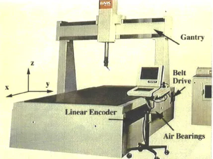
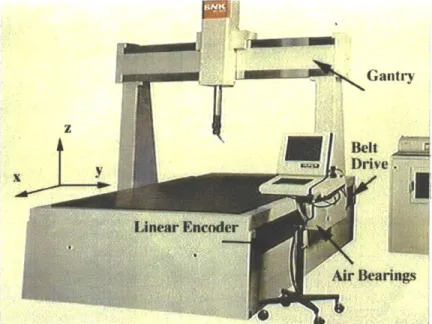
1.4 _{Overview of the coordinate measuring machine (Courtesy of SNK Co.,} Ltd) ... ... ... 17

1.5 Symmetric Root locus of the LQR design . . . . 18

1.6 Desired asymmetric root locus for the coordinate measuring machine that gives good stability properties, high speed of response and other performance/robustness properties. . . . . 19

1.7 Setup for robust estimation problem. . . . . 20

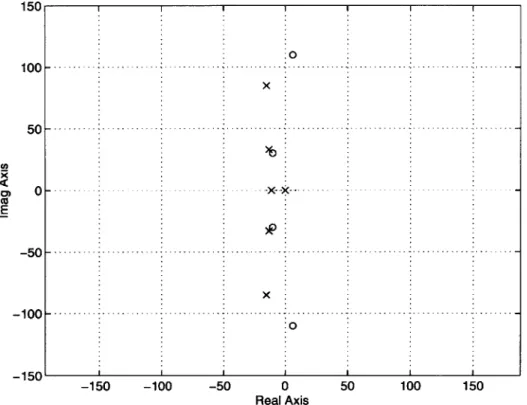
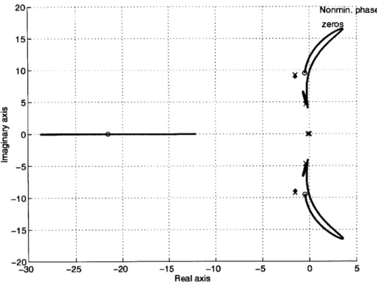
2.1 Example of nonminimum phase system with zeros close to the imagi-nary axis (Pole-zero plot of Coordinate Measuring Machine described in Sections 2.4 and 2.5). . . . . 26

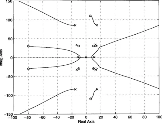
2.2 Symmetric root locus for the example system. . . . . 27

2.3 Asymmetric root-squared locus. . . . . 28

2.4 _{Overview of the coordinate measuring machine (Courtesy of SNK Co.,} Ltd) ... .. ... ... 37

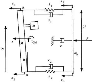
2.5 Schematic diagram of the x-axis drive system. . . . . 38

2.6 Effect of change in location of mass m on the poles and zeros . . . . . 39

2.7 Bode plot fit for the Coordinate Measuring Machine . . . . 40

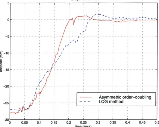
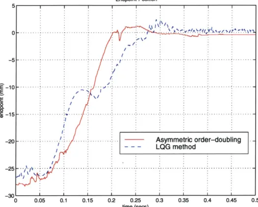
2.8 Comparison of the endpoint position of LQG method with Asymmetric order-doubling method. . . . . 43

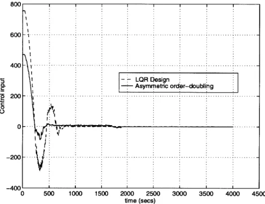
2.9 Comparison of the endpoint position of LQG method (with larger gain) with Asymmetric order-doubling method. . . . . 2.10 Control inputs used by LQR and Asymmetric order-doubling

approa-ches for p = 0.5. . . . . 2.11 Comparison of tracking using asymmetric order-doubling and LQ servo

m ethods (p = 0.5) . . . . 2.12 Nyquist plot for the LQR method. Note that the plot doesn't enter

inside the unit circle centered at (-1,0). . . . .

2.13 Nyquist plot for the Asymmetric order-doubling method. . . . .

2.14 Comparison of Sensitivities of the LQR method and the Asymmetric order-doubling approach. . . . .

2.15 Comparison of Complementary sensitivity funtions of the

and the Asymmetric order-doubling method. . . . .

3.1 Simple block diagram for M. . . . .

3.2 Partitioned representation of M. . . . .

3.3 Block diagram for A. . . . . 3.4 Lower linear fractional representation of M and A.

3.5 Upper linear fractional transformation of M and Q.

3.6 LFT representation of uncertain parameter c. . . . . . 3.7 LFT representation of an uncertain parameter c-1

.

3.8 Schematic diagram of the y-axis drive system. . . . . .

3.9 Simulation of endpoint position of CMM for a nominal

LQR method

. . . . 5 1 . . . . 58 . . . . 58 . . . . 59 . . . . 59

. . . .

60

. . . . 6 1

. . . .

62

. . . .

64

system using asymmetric order-doubling with standard Kalman filter. . . . .

3.10 Simulation of states of CMM for a nominal system and comparison with

the state estimation results when we use asymmetric order-doubling with standard Kalman filter. . . . .

3.11 State estimation errors for a nominal CMM system when we use a

standard Kalman filter. . . . . 44 45 46

48

49

50 65

66

67

3.12 Simulation of endpoint position of a perturbed CMM using asymmetric

order-doubling with standard Kalman filter. . . . . 68

3.13 Simulation of states of a perturbed CMM and comparison with the state estimation results when we use asymmetric order-doubling with standard Kalman filter. . . . . 69

3.14 State estimation errors for a nominal CMM system when we use a standard Kalman filter. . . . . 70

3.15 Nominal system response during regulation using asymmetric order-doubling and standard Kalman filter. . . . . 71

3.16 Perturbed system response during regulation using asymmetric order-doubling and standard Kalman filter. . . . . 72

4.1 Setup for standard filtering problem. . . . . 77

4.2 Setup for robust filtering problem. . . . . 90

4.3 Setup for robust filtering problem. . . . . 121

4.4 Linear System G, . . . . . . 123

4.5 Endpoint position and its Estimate using robust Kalman filtering . . 127

4.6 Comparison of standard filtering and robust filtering approaches for the nominal system . . . . . 128

4.7 Comparison of standard filtering and robust filtering approaches for the perturbed system. . . . . 129

4.8 States and state estimates of the nominal system using robust Kalman

filter. . . . .

130

4.9 States and state estimates of the perturbed system with robust Kalman filter. . . . . 13 1 4.10 State estimation errors for nominal system using robust Kalman filter. 132 4.11 State estimation errors for a perturbed system using robust Kalman

filter. . . . .

13 3

4.12 Bode plots of robust Kalman filter and standard Kalman filter . . . . 134

4.13 Nominal system response during regulation using asymmetric order-doubling with (a) standard Kalman filter and (b) robust Kalman filter. 136 4.14 Perturbed system response during regulation using asymmetric

order-doubling with (a) standard Kalman filter and (b) robust Kalman filter. 137 4.15 Another perturbed system response during regulation using

asymmet-ric order-doubling with both standard Kalman filter and robust Kalman

filter. . . . .

139

4.16 Comparison of standard Kalman filter for the nominal and two per-turbed system s. . . . . 140 4.17 Comparison of robust Kalman filter for the nominal and two perturbed

Chapter 1

Introduction

In

this thesis, we consider a class of nonminimum phase systems that have zeros close to the imaginary axis and address the problem of controlling such systems in the face of uncertainty. This class of physical systems is rather important and is quite common in a wide variety of practical applications. The research was mainly motivated by studying a set of industrial machines like coordinate measuring machines

(CMM), numerically controlled (NC) machines, milling machines, digitizing machines,

laser cutting machines, drilling and boring machines etc. The two main important features in the applications for which this thesis provides a satisfactory control design method (from both theoretical and practical standpoint) are: firstly, the systems have nonminimum phase zeros and secondly, there are uncertainties and nonlinearities that degrade the performance of the system.

The first feature, namely, the presence of nonminimum phase zeros, is an un-desirable feature of the system. These nonminimum phase zeros appear due to the noncollocated location of sensors and actuators. For the several practical applications listed earlier, these nonminimum phase zeros cannot be avoided because of our choice of endpoint sensor. The study of such systems has been a topic of active research for several decades both theoretically and practically. Recently, the control of nonmini-mum phase systems has become increasingly important in many applications. This has revived the subject of control design of nonminimum phase systems. Greater emphasis has been given to the development of practical and implementable design

methods for such systems, that has a theoretical foundation as well. High speed coordinate measuring machines or NC machines, for example, exhibit nonminimum phase behavior due to the coupled rotation and translation of its gantry structure and due to the noncollocated sensor/actuator configuration. Also, endpoint feedback of machine tools and robots give rise to nonminimum phase control problems in many situations. Due to the structural deflection, the endpoint dynamics often show a sig-nificant undershoot. A large phase lag incurred in the endpoint feedback loop due to this may destabilize the system. Despite these increasing needs, the control design of nonminimum phase systems still remains as a difficult problem. The difficulty of such systems is enhanced by the presence of inherent performance limitations for such systems.

The second feature, namely, presence of uncertainties and nonlinearities that de-grade the performance of the system, is an important issue in most practical applica-tions. Over the last two decades, special attention has been given to the robustness issues of such systems. Several theoretical developments leading to p-analysis (see [4]) and a generalization of it to include nonlinearities, called the integral quadratic con-straints approach (see [24]) have been developed. The design methods developed, however, are not quite satisfactory. They, typically, tend to decrease the gain of the controller in order to achieve good robustness properties. This will decrease the speed of response considerably. Hence, there is a compromise between high perfor-mance and good robustness for such systems. It is, therefore, desirable to develop a robust control method that does not decrease the gain of the system, yet provide

some robustness in the design.

There are a variety of applications which have both the above features. Some of them are, as mentioned earlier, coordinate measuring machines, NC machines, dig-itizing machines, laser cutting machines, milling and boring machines, arc welding robots, etc (see Figure 1.1, 1.2 and 1.3). This thesis addresses all of these appli-cations and provides a control design method that achieves very high performance for such systems. In this thesis, we demonstrate the results not only through the theoretical guarantees and simulation results, but also through experimental results,

by implementing the design method to an industrial coordinate measuring machine

shown in Figure 1.4. We also show a clear agreement of the theoretical results and simulations with that of the experimental results thereby confirming the advantages of the new control design method.

(a) 3-axis milling machine. (b) High speed milling machine.

Figure 1.1: Applications (Courtesy of SNK Co., LTD).

First, a new control design method is developed for the nominal system called the asymmetric order-doubling method. For the nominal system, traditional pole placement methods are often not suitable to obtain satisfactory controllers in dealing with nonminimum phase zeros. Linear quadratic regulator (LQR), when combined with Kalman filtering, provides a design procedure ([1, 11, 13, 16]) that is applicable to nonminimum phase systems. But it is difficult to explore the entire class of optimal state feedback gains that are parametrized by the weight matrices of the performance index. Further, the robustness properties with respect to the various descriptions of uncertainties are not well handled by these design methods. The symmetric root locus method of LQR provides a class of optimal controllers parameterized by one scalar weight p describing the relative magnitude of the regulation error to the control input. Namely, the optimal state feedback gains are given by the stable part of the symmetric root locus

([17]).

This method is simple, easy to comprehend and allows

(a) Vertical drilling and boring machine. (b) Ultra sonic knife cutting machine.

Figure 1.2: Applications (Courtesy of SNK Co., LTD).

the designer to gain useful insights in the resulting control system (see Figure 1.5). However, it exploits only a fraction of possible solutions ([2]). It is particularly unsatisfactory when the given plant contains nonminimum phase zeros and unstable poles close to the imaginary axis. These poles and zeros, when reflected to the mirror image (to get the closed loop poles of LQR design), remain close to the imaginary axis even at high control gains. They dominate the system behavior and slow down the system response. The symmetric root locus, therefore, confines the optimal state feedback gains within the symmetric mirror image, but other desirable solutions may exist at asymmetric locations (like, for example, Figure 1.6).

In this thesis, we first generalize the symmetric root locus approach by allowing asymmetry in the root locus with respect to the imaginary axis. Note that in

Fig-ure 1.5 the left half plane (LHP) is a mirror reflection of right half plane (RHP) unlike

Figure 1.6. This new approach is expected to be a practical and powerful design tool for unstable and nonminimum phase systems. As mentioned earlier, this allows the designer to pick the stable LHP portion with the dominant poles further away from the imaginary axis (see Figure 1.6 and compare with Figure 1.5) giving a faster speed of response. The effectiveness of this method will be demonstrated by applying it to

(a) Digitizing machine. (b) Laser cutting machine.

Figure 1.3: Applications (Courtesy of SNK Co., LTD).

a 3D-coordinate measurement machine, which exhibits nonminimum phase behavior (see [30]). The new method is also shown to have good stability margins compared to the LQG method.

The next objective is to achieve good robustness against parametric uncertainties while maintaining the high performance achieved through asymmetric order-doubling method. As mentioned earlier, the current robust control design methods like I-synthesis decrease the gain of the system (compromising the performance) in order to achieve good robustness. To achieve both good performance and good robustness requires a detailed study of the various sources of uncertainty. It will be seen that parametric uncertainty is an important source for the degradation of performance in these systems. This source of uncertainty for the coordinate measuring machine comes from the dynamics of the air bearing and variation of the belt stiffness. It will be seen that the asymmetric order-doubling method does not have good robustness with respect to this type of parametric uncertainty. From careful analysis through simulations and experiments, it will be seen that the state estimation errors become significantly large. This is the main reason for the degradation in the performance of the perturbed system, although the nominal system has high performance.

Gantry

Belt C

y

~1Drie.

Linear Encoder

ArBearings

Figure 1.4: Overview of the coordinate measuring machine (Courtesy of SNK Co.,

Ltd)

From the Youla parametrization

([36])

of all stabilizing controllers for a given system, it is apparent that any control problem has two important subproblems: full information control problem and a state estimation problem. For a linear system, there is a clear separation structure between these two subproblems i.e., solving both the subproblems separately gives a solution to the original control problem. This, however, is not true for an uncertain or an nonlinear system. Some form of iteration between these two subproblems is required to obtain a satisfactory controller for such systems. The asymmetric order-doubling control can be considered as an example of full information control problem.

From the analysis, it will be seen that poor state estimation is responsible for degradation in performance for the perturbed systems. We will rectify this situation

by designing a robust state estimator and will use the previously designed asymmetric

order-doubling control as the full information control subproblem. The objective of a robust state estimator is to minimize the effect of disturbances and exogenous noise on the state estimation errors. Figure 1.7 shows the setup for a robust state estimator design. G(s) represents the plant, A the uncertainties and nonlinearities, H(s) the estimator that we need to design, wo the exogenous noises and e the state estimation

- 5 0 - . .. ... . .. ---.. .. -. ... .---. .. .. .. -.--- -.-.-.-.-. .-.-.

- 10 0 --. ----. -.

--.--.--150

-100 -80 -60 -40 -20 0 20 40 60 80 100

Real Axis

-10

-100 -80 -60 -40 -20 0 20 40 60 80 100

Real Axis

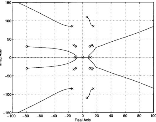
Figure 1.6: Desired asymmetric root locus for the coordinate measuring machine that gives good stability properties, high speed of response and other perfor-mance/robustness properties.

errors. The objective is to design H(s) such that the norm from the inputs wo to the outputs e is minimized. In this thesis, we will consider the class of uncertainties and nonlinearities that can be represented in terms of integral quadratic constraints (IQC's). It has been shown that several uncertainties and nonlinearities like time-varying gains, backlash, dead-zone, saturation, sector nonlinearities, norm bounded uncertainties, rate limiters, etc have been represented as IQC's effectively (see [24]).

In this thesis, we use this framework and give a solution to the robust estimation problem by representing it as linear matrix inequalities (LMI's). This LMI represen-tation is convenient since the primal-dual algorithms solve these problems efficiently in polynomial-time (see

[26]).

It will be shown experimentally that this approach not only improves the state estimation errors but it also improves the performance of the perturbed system for the CMM.

'

yzz

W1

G(s)

- H(s)

Il

A

Figure 1.7: Setup for robust estimation problem.

1.1

Organization of the Thesis

In Chapter 2, the asymmetric order-doubling control method is explained in detail. The theoretical derivations of the basic asymmetric order-doubling method is de-veloped first. As an application of the method, an industrial coordinate measuring machine is considered. The new method was implemented on the machine and was compared with the LQG method. Significant improvement in the speed of response

will be demonstrated. The robustness properties in terms of stability margins, sen-sitivities, complementary sensitivities are discussed and compared with that of the

LQG method and will be shown to be quite similar.

In Chapter 3, the sources of parametric uncertainty is discussed. It will be shown that the asymmetric order-doubling controller does not have good robustness prop-erties in terms of uncertain parameters like belt stiffness, air bearing stiffness and damping. It will be identified that the state estimation is degraded considerably due to the uncertainty in the parameters. This will be shown to be the main source of degradation of performance of the perturbed system.

In Chapter 4, a robust state estimator will be designed with an objective of im-proving the state estimation for the perturbed system. The uncertainty description considered is more general and allows for nonlinearities as well. More specifically, the uncertainties and nonlinearities described in terms of integral quadratic constraints is considered. A robust state estimator is designed and is shown to be a convex

optimization problem. A linear matrix inequality representation is derived to rep-resent the convex optimization problem in a numerically tractable way. The robust filter will then be shown to improve the state estimation considerably. Experimental results will demonstrate the improvement of performance for both the nominal and perturbed systems using the new robust filtering approach combined with asymmet-ric order-doubling control. The experiments were conducted by changing the belt stiffness and the air bearing pressure (which is reflected as changing the air bearing stiffness and damping properties). For this perturbed system, the improvement of performance as well as state estimation will be demonstrated.

Chapter 2

Asymmetric Order-Doubling

Control Design

2.1

Introduction

Control of nonminimum phase systems is becoming increasingly important in many practical applications. High speed coordinate measuring machines, for example, ex-hibit nonminimum phase behavior due to the coupled rotation and translation of its gantry structure and due to the noncollocated sensor/actuator configuration. Also, endpoint feedback of machine tools and robots gives rise to the nonminimum phase control problems in many situations. Due to the structural deflection, the endpoint dynamics often shows a significant undershoot. A large phase lag incurred in the endpoint feedback loop due to this may destabilize the system.

Despite the increasing needs, the control design of nonminimum phase systems still remains as a difficult problem. Traditional pole placement methods are often not suitable to obtain satisfactory controllers in dealing with nonminimum phase zeros. LQR, when combined with Kalman filtering, provides a design procedure ([1, 11, 13, 16]) that is applicable to nonminimum phase systems. But it is difficult to explore the entire class of optimal state feedback gains that are parametrized by the weight matrices of the performance index. This is a serious drawback in most of the modern optimal control methods like H2 and H' designs. There are only a few

guidelines to choose the weighting matrices in these optimal control methods in order to get a good performance. These guidelines are not quite satisfactory for systems with nonminimum phase zeros close to the imaginary axis. Further, the performance specifications are usually expressed in frequency domain rather than time-domain conditions like rise time, settling time etc.

The symmetric root locus method of LQR provides a class of optimal controls parameterized by one scalar weight p describing the relative magnitude of the regu-lation error to the control input. Namely, the optimal state feedback gains are given

by the stable part of the symmetric root locus

([17]).

This method is simple, easy to comprehend and allows the designer to gain useful insights in the resulting control system. However, it exploits only a fraction of possible solutions ([2]). It is par-ticularly unsatisfactory when the given plant contains nonminimum phase zeros and unstable poles "close" to the imaginary axis. These poles and zeros, when reflected to the mirror image (to get the closed loop poles of LQR design), remain close to the imaginary axis even at high control gains. They dominate the system behavior and

slows down the system response. The symmetric root locus, therefore, confines the optimal state feedback gains within the symmetric mirror image, but other desirable

solutions may exist at asymmetric locations.

In this chapter, we will generalize the symmetric root locus approach to a class of asymmetric root loci using basic properties of "order-doubling" techniques. The new method is expected to be a powerful design tool for unstable and nonminimum phase systems. The effectiveness of the method will be demonstrated by applying it to a 3D-coordinate measurement machine, which exhibits nonminimum phase behavior

(see [30]).

In Section 2.2, the basic concept of asymmetric order doubling will be introduced

by giving necessary definitions and properties. The new method will be compared

with other methods such as LQR and loop transfer recovery (LTR). In Section 2.3, the underpinning theory for the asymmetric order-doubling method will be presented, and a computational procedure for obtaining stable state feedback gains will be developed. In Section 2.4, the control of a coordinate measuring machine will be considered as

an application of this method. In Section 2.5, the experimental results comparing regulation with that of the LQG method will be presented. Significant improvements

have been obtained in the speed of response, while using lower control inputs than that of the LQG method. In Section 2.6, the performance and robustness characteristics of this method will be discussed and will be shown to be comparable to that of the LQR method. Furthermore, it will be shown that this method would improve the speed of response while maintaining stability, nominal performance and robustness of that of the LQR method, particularly for systems with nonminimum phase zeros close to the imaginary axis. In addition, it will be demonstrated that this new method will use smaller control inputs to achieve these objectives and will be easier to implement.

2.2

Asymmetric Order Doubling Method

Consider an n-th order multi-input, multi-output (MIMO) linear time-invariant (LTI) system represented by

z(t)

= Aix(t) + Biu(t),

_(2.1)

y(t) = Cix(t),

where

[A

₁, B1

]

is assumed to be stabilizable and

[A

1, C1] to be detectable. The system

may be unstable and/or be of nonminimum phase.

The design procedure and basic properties of the asymmetric order-doubling method will first be provided for single-input single-output (SISO) systems for the sake of clarity and physical intuition. Later, these definitions will be extended to

MIMO systems.

Definition 2.1 Given an LTI system described by Equation (2.1), order-doubling

is defined as the procedure in which the same number of poles and zeros as that of the

open loop plant are added in such a way that the resultant order-doubled system has

the same number of poles and zeros in both the LHP and the RHP.

the gain as

(-1)d,

where d = number of poles

+

number of zeros of the open loop

system, is termed as the root-squared locus of the original system. The parameter

along the root-squared locus is called the locus parameter, p; 0 ; p

<

oo.

Definition 2.3 If all the branches of the root-squared locus obtained by a suitable

order-doubling of the system do not cross the imaginary axis, then this particular

order-doubling procedure is said to satisfy the separability condition.

When separable, all the branches of the root-squared locus never cross the imag-inary axis. As an analogy, in terms of these definitions, the root-squared locus of the LQR design is separable and is symmetric with respect to the imaginary axis. Hence it is called a symmetric root locus. It is a fact that in the LQR design, the root-squared locus is always "separable" and that it is possible to extract only the LHP portion of it as a unique positive semidefinite solution of a certain matrix Riccati equation. The Schur method

([18])

is one of the numerically stable methods for determining this solution. The corresponding control then becomes a stable state feedback. This concept is used in the LTR procedure to create a model-based compensator which allows the dynamics to be changed to some desired dynamics whenever the plant is

of minimum phase

([3,

33]).

The LQR design based on the symmetric root locus, however, may incur unde-sirable behavior for a class of systems with nonminimum phase zeros. Consider the pole-zero plot shown in Figure 2.1. Since a pair of nonminimum phase zeros are lo-cated close to the imaginary axis, the branches of the symmetric root locus indilo-cated in Figure 2.2 tend to go close to the imaginary axis. Note that the two branches of the root locus approach the "fictitious" zeros in LHP, which are the mirror image of "real" nonminimum phase zeros. These zeros do not exist physically but were introduced for the purpose of computational convenience. The closed loop poles approaching the fictitious zeros are not attenuated by the real zeros and, therefore, exhibit a slow oscillatory mode. To resolve this problem, the fictitious zeros must be placed further from the imaginary axis. This makes the root-squared locus asymmetric, as shown in

150 100 | - ---. --- - -- --50H .... 0 -10 0 - --. ---. ---. -150 -100 -50 0 50 100 150 Real Axis

Figure 2.1: Example of nonminimum phase system with zeros close to the imagi-nary axis (Pole-zero plot of Coordinate Measuring Machine described in Sections 2.4 and 2.5). An CM E

-X-~

.. .. . ... .. .. .. . x - - -- - -- --- ---- --150 -50 -

--E - 5 0 - -. .. .- ----.. - -- --.-..-.- -.-- -.-..--.--.-. .. .-. .- -. - 10 0 --- ---- - -- - - - - -- -- --150' -100 -80 -60 -40 -20 0 20 40 60 80 100 Real Axis

In Figure 2.3, all the root locus branches in LHP are pushed away from the imag-inary axis, making the dominant poles faster. The focus of this chapter is to obtain conditions under which this asymmetric root locus provides a stable state feedback control. The main part of the conditions is given by the separability condition stated in Definition 2.3. It will be shown in the following section that, if the root-squared locus is separable into LHP and RHP, there exists a stable state feedback control that locates the closed loop poles on the LHP portion of the root-squared locus. Under this separability condition, a modified algebraic Riccati equation will be solved to obtain the stable controller.

150 100 50 0 A2 E -50 -100 -1 5 01 - 1 1 1 -100 -80 -60 -40 -20 0 20 40 60 Real Axis

Figure 2.3: Asymmetric root-squared locus.

The general procedure for designing state feedback control based on this asym-metric order doubling is as follows:

1. For the transfer function matrix of a given plant, plot the poles and zeros on

the complex plane.

2. Perform order-doubling by placing the same number of poles and zeros as that of the open loop system.

3. Obtain the root squared locus for this system.

4. If the root-squared locus is separable into the LHP and the RHP, each containing n poles, then form a matrix Riccati equation, and solve it to get the state feedback controller (as described in Theorems 2.1 and 2.4).

The underpinning theory for this procedure will be given in the next section and the method will be applied to a practical system in Sections 2.4 and 2.5.

2.3

Theoretical Results

Let G'L(s) = C1(sI - A1) -1B1 be the tranfer function matrix of the open loop plant

and G2OL s 2(sI - A2)'B 2 the transfer matrix associated with the additional

poles and zeros. The asymmetric root-squared locus of the combined system can be obtained by solving for the roots of the following equation:

det I + -G

21

L(-s)G

=(s))

0.

(2.2)

For a SISO case, this reduces to the familiar root locus equation:

1 n

2

(-s) ni(s)

-o

(2.3)

pd2(-s) di(s)

where G' (s) = ni(s)/di(s) and G0(s) =n 2

(s)/d

2

(s).

This 2nth order system will be expressed as a product of two nth order systems. Further, the two nth order systems will be chosen in such a way that one correspond to the LHP and the other to the RHP, whenever possible. This decomposition would allow us to compute the state feedback control inputs from the solution of a modified Riccati equation. The stable LHP portion would then correspond to the closed loop poles. The following theorem first introduces the modified algebraic Riccati equation, the solution of which is required later to construct the state feedback control gain.

Theorem 2.1 Let (A

1

, B

1

, C

1

) be a minimal realization of an open-loop transfer

func-tion matrix Gb(s)

C1(sI

-

A

1

)-'B

1

. Let (A

2

, B

2

,C

2

) be a minimal realization of

G2L(s) =2(sI - A₂) B2 that is added to the original plant to generate an

order-doubled system. The condition that the matrix K is an arbitrary solution to the

Modified Algebraic Riccati Equation (MARE) given by

1

KA

1

+ A'K +C2C1

-

-KB

1

BfK = 0,

(2.4)

2

~

P 2

is equivalent to the decomposition condition given by

1

I + -GO

L

(-sGOL(s)

=

[I

+

GAO(-s)][I+

GAO(s)],

(2.5)

p

where G1

0

(s)

G1(sI

-

A

1

)-

1

B

1

and G2O(s) = G

2

(sI

-

A

2

)-'B

2

with G

1

(1lp)B'K and G' = (1/p)KB1.

Proof: Rewriting Equation 2.5 by substituting all the transfer matrices gives

1

I

+ -B (-sI

-

A

)-'C'C1(sI

1

-

A1)-'B1

[I + B (-sI

-

A)-

1

'2][I + G1(sI

-

A

₁

)-

1

B

₁

], (2.6)

Expanding the right hand side of this equation and simplifying it,

1 1

RHS =I + -B (-sI

-

A

-KB

1 1

+ -BIK(sI

-

A

1

f)B

1

+

P P

1

- B(-sI-

A')

KB1B K(sI

-

A

1

'B

1

, (2.7)

p

since G1 =

(1/p)B'K

and G' =

(1/p)KB1.

Cancelling the common terms on both

sides of Equation 2.6 and grouping the other terms together,

B (-sI

-

A')

C C1 + KA

1

+ A'

2

K

-

-KB1B

K (sI

-

A

1

)'B

1

= 0.

steps can be carried out in the reverse order to complete the proof of the theorem. E Note that the matrix K in the above theorem does not necessarily provide a physically realizable, stable control. To obtain a stabilizing controller for the system, a physically meaningful solution K of MARE should be solved whenever it exists. To this end, the solutions of MARE must be examined in order to guarantee the existence of such a solution. The following lemma is needed to represent the solution.

Lemma 2.1 The Hamiltonian matrix H defined by

H =

(2.8)

H

-(

1

-

A/

is similar to

SA

1

-

B

1

G

1

--LB1B'

H

=

(2.9)

0

-(

A2- B2G2)'

under the similarity transformation (i.e., HI = T-1HT)

I

0

T =

(2.10)

(K I

when K is any solution to the modified algebraic Riccati equation given by

Equa-tion (2.4) and G

1

= (1/p)B'K, G' = (1/p)KB1. Further, the closed loop poles,

ob-tained by choosing u(t) =

-G1

x(t), are 'n' of the 2n eigenvalues of the Hamiltonian

H.

This lemma can be proven simply by calculating T- 1HT for T given in Equa-tion (2.10). In the following theorem, all the soluEqua-tions of MARE will be characterized and this would generalize the results of Potter [29], Martensson [19] and Kucera [15]. Note that the previous works dealt with standard Riccati equations where matrices A1

and

A

2 are the same, while in this chapter

Ai

/

A

2 due to the asymmetric nature of

the order-doubled systems. Here Ai

$

A2 is not just a mathematical generalization,

the plant dynamics as opposed to just one way, through the familiar loop transfer recovery method. It also gives a systematic way of calculating the root locus branches numerically for a large class of systems. The solutions K of the MARE are expressed in terms of the eigenvectors of the Hamiltonian H.

Theorem 2.2 Let ti be the 2n-dimensional eigenvector of Hamiltonian H given by

Equation (2.8) corresponding to the eigenvalue Ai and let

ti =A

Lqi

(2.11)

where pi and qi are n-dimensional vectors. Then, every solution of Equation (2.4)

can be expressed as

K = [q1... q] [p1... pn]--

(2.12)

where the inverse of [p1 ...

p,,]

is assumed to exist

for

certain combinations of eigen-vectors ti. Conversely, if

[P1

... pn] is nonsingular, then

K = [q1... q.][p1 ...

pn]--satisfies Equation (2.4).

Proof: Let K be a solution of Equation (2.4) and define

1

Ac, =

A

1 -

-B

1

B1K

p

(2.13)

(this is the closed loop system matrix - see also Lemma 2.1). Premultiplying Ac, by K gives

1

KAci

=

KA

1 -

IKB

1

B K,

P

which from Equation (2.4) becomes

Let T be the transformation that takes Ac, into a

Define S = KT. Then

Jordan form

J

i.e.,

T

1

AcT = J.

Ac,

_{TJT ',}

K = ST-

1

.

(2.16)

Substituting these in Equations (2.13) and (2.15),

[J]

A

L

I-C2C 1

-

1

B

1

B'

T

T

P

=

H

. -A' 2p S S

(2.17)

Let ti,... , tn be the columns of the 2n x n matrix

T

S

(2.18)

It follows from Equation (2.17) that these column vectors constitute the eigenvectors of H and that the corresponding eigenvalues are also the eigenvalues of Ac,. Fur-thermore, the above statement is true if the eigenvalues have multiplicities greater than one (see [19]). In this case, all of the generalized eigenvectors are present in the column vectors ti,... , tn. Finally, from Equation (2.16) we have (see Equation 2.11)

K = [q

..

.qn][pI ... pn]-.

(2.19)

The converse is proved by carrying out the steps above in the reverse order. This completes the proof of the theorem.

Corollary 2.1 Let ti, i = 1, . . . , n be eigenvectors of H corresponding to A,, .. ,An.

If K = [q1 ... qn][p1 ... pn] 1 is a solution of Equation (2.4), then

A,,...

,

An

are the

eigenvalues of

[A

1 -

(1|p)BIB'K]

and p,... ,pn are the corresponding eigenvectors.

The theorem below gives conditions for the solution K to be real, the proof of which is along the same lines as Theorems 3 of Martensson [19]. These conditions for the solution K to be real will be used to construct a physically realizable control input that can stabilize the closed loop system.

Theorem 2.3 The necessary and sufficient conditions for a solution

K = [q1... q.] [p1... pn]-1

(2.20)

to be real are

(i) all eigenvectors

t

₁

,...

,

tn are real, or

(ii) if ti of rank k corresponding to the eigenvalue Ai, Im(Ai) / 0, is used to construct

the solution K, then ti (complex conjugate of ti) of rank k corresponding to Ai

(complex conjugate of Ai) must also be included in the solution.

The next main theorem provides conditions for the existence of a stable state feedback control.

Theorem 2.4 (Separability):

Under the assumptions stated in Theorem 2.1,

there always exists a solution K of the MARE such that the state feedback control

formed as u(t) = -(1/p)B'Kx(t) guarantees all the closed loop poles to lie in the

stable LHP whenever the separability condition is satisfied.

From the separability theorem, the closed loop poles are given by 1

1 +

-B

K(sI

-

A

1

) 'B

1

= 0.

(2.21)

p

An alternative to solving the above equation is to obtain the eigenvectors of the Hamiltonian H corresponding to the n LHP eigenvalues as stated in Theorem 2.2. An important consequence of the above theorems is the following corollary which can

be used to prove the LTR asymptotic property for minimum phase systems. This

Corollary 2.2 If K exists as specified in Theorem 2.4 to Equation (2.4), then the

closed loop poles move as follows:

(i) As p

-+

oo, the closed loop poles start at the stable open loop poles or at the

mirror image of the unstable open loop poles,

(ii) As p

--

0, the closed loop poles move to cancel the minimum phase zeros, go to

the mirror reflections of the nonminimum phase zeros or approach oo on either

side of the imaginary axis.

Next, the LTR asymptotic property that gives us a design procedure for stably in-verting the dynamics of the plant when used with a model based compensator will be discussed. This extends the well-known LQG/LTR method ([3, 33]) to a broader class of systems. The proof is along the same lines as for the LQG/LTR method described in [2].

Theorem 2.5 If C1(sI

-

A

1

)-

1

B

1

is minimum phase, then

lim VI G1

W C1,

(2.22)

for

some orthogonal matrix W, i.e., WTW I.

In summary, the LQR controller sends the poles to the stable LHP portion by mirror reflecting about the imaginary axis if necessary, whereas the asymmetric controller sends the poles to any location in the LHP in an exactly analogous way. It is possible to maintain most of the robustness properties of the LQR design by staying close to the LQR solution.

Until now, all the results have been considered for SISO, even though the mathe-matical derivations do not require to be SISO. To extend this naturally for both SISO and MIMO systems, the definitions will be modified so that the theoretical results will still hold. Definition 1 of order-doubling is applicable to MIMO systems without any modification.

Definition 2.4 Root-squared locus is termed as the locus of the roots of the

order-doubled system given by the following equation, when p changes from 0 to oc:

det [I +-G

L(-s)Go'(s) = 0,

(2.23)

where G'L(s) is the transfer function matrix of the original open loop plant and

G2L (s) is that for the additional poles and zeros added during order-doubling. The

parameter along the root-squared locus is termed as the locus parameter, p.

Definition 2.5 If none of the roots of Equation (2.23) lie on the imaginary axis for

all values of p in (0,

oo),

then this particular order-doubling procedure is said to satisfy

the separability condition: separated into LHP and RHP.

2.4

Application

2.4.1

The System

The control of a 3D-coordinate measuring machine (CMM) is considered as a practical example of a nonminimum phase system. All experiments were conducted on the CMM shown in Figure 2.4.

The large gantry shown in the figure is driven along the x-axis by a servo mo-tor through pulleys and steel belts on both sides of the table. To reduce friction, air bearings are used for supporting the gantry. Figure 2.4 shows the schematic of the lumped parameter model of the x-axis drive system. Mass M with centroidal moment of inertia, Ic, represents the gantry, while mass ma is the actuator-side inertia including the effective inertia of the motor rotor and gearing. Drive force F generated by the actuator is transmitted to the gantry M through two steel belts modeled as stiffness ki, k2 and damping

ci,

c2, respectively. The stiffness on each side

of the steel belt may differ, since the stiffness significantly varies depending on the belt tension. Also, the mass centroid of the gantry shifts along the y-axis depending on the location of the y-axis moving part denoted by mass m. This asymmetrical

Gantry Belt

Drive ,a A*

Air Bearings

Figure 2.4: Overview of the coordinate measuring machine (Courtesy of SNK Co.,

Ltd)

mass property along with the asymmetrical belt stiffness causes the gantry to rotate when pushed by the belts. As a result, the motion of the gantry exhibits the behavior of a nonminimum phase system, i.e., undershoot, when observed by a linear encoder measuring the x-coordinate of point A or B, x1 or x2. Namely, a sudden rotation of

the gantry may instantaneously push either side of the gantry backward, hence an undershoot occurs.

The equations of motion concerning the translation x and rotation 0 of the gantry as well as the motion of the motor-side inertia, X3, are given by

(M + m)i + (c

1

+ c

2

)± + (k

1

+

k

2

)x + (cll1

-

c

2

1

2

)$ + (k

11

-

k

2

l2)0

=

(c1 + c2)i3

+

(ki

+

k2)X3,

IcmN + (c1l

+

c

2

li) + (k

1

l? + k

2

li)9 ± (c2i1

-

c

2

1

2

)± + (k

11

-

k

2

l

2

)x =

(cili - c212)i3 + (kili - k22)3,

maia =

F -

(M

+

m)z - ci.

The output is the coordinate x2 given by x2 = x - 120. Figure 2.6 shows the

x 3 xI x 2 _x 3

Figure 2.5: Schematic diagram of the x-axis drive system.

m is varied, their loci are shown as functions of the y coordinate. One interesting observation to make is when the mass m is at the bottom. The center of mass is then lower and the combined translation and rotation of the mass M causes it to turn counterclockwise at the location B. In other words, the system tends to be a nonminimum phase system as illustrated in Figure 2.6 (the zeros move into the right half plane). When the mass m is in the middle, the applied force F is acting almost at the center of mass. Therefore, the rotation of the mass M is not quite observable at B. This causes a near pole-zero cancellation as shown in Figure 2.6. The situation becomes more apparent if the spring stiffness on both sides are different.

2.4.2

Identification

Frequency response tests were performed in order to verify the analytical model ob-tained above. The results are shown in Figure 2.7. At about 90 rad/sec, the magni-tude plot shows that the slope is at -80 dB/decade while the phase plot shows that the phase angle is about -270'. This implies that the magnitude and phase do not correspond as they would for a minimum phase system. The pole-zero plot shown in Figure 2.1 was that of the CMM, which illustrated the nonminimum phase behavior.

2 0 - --.---. --- .

-20 -15 -10 -5

Real axis

0 5

Figure 2.6: Effect of change in location of mass m on the poles and zeros

2.5

Implementation and Experiments

2.5.1

Control Tuning

The asymmetric order doubling method was implemented on the CMM based on the dynamic model obtained in the previous section. As described in Section 2, the first step of control tuning is to plot the pole-zero map of the system and perform order-doubling by placing the same number of additional poles and zeros. The question is where to locate these additional poles and zeros. As initial locations of the poles and zeros, we choose them to be that of the LQR design, i.e., the mirror image locations of the plant's poles and zeros. This guarantees the separability condition to be always satisfied. However, as emphasized earlier, this choice is not good for systems with nonminimum phase zeros close to the imaginary axis since it gives a slower time response. Hence, the zeros must be relocated further away from the mirror reflection of the system zeros and also away from the imaginary axis. The poles can be placed close to the mirror reflection of the system's poles to maintain the separability and

K

- - - - --

---15 10 -.. ... .. .Nonmin.phase zeros ------

---C - -

-..... . . .. . .. . .. . . .. . .. . . 5 0 -5 as E -10--15 -20 -30 - . --25

I

20

slope: -80 db/ c

20

--- - Experimental data 40 Bode plot fit

40 rAA 10 1 Frequency (rad/sec) 102 102 10 1 Frequency (rad/sec)

Figure 2.7: Bode plot fit for the Coordinate Measuring Machine

- C-100 0) 4) (L -360 10