Analysis of multiphase fluid flows via high speed and synthetic aperture three dimensional imaging

(1)

Analysis of Multiphase Fluid Flows via High Speed and Synthetic Aperture Three Dimensional Imaging

by

Barry Ethan Scharfman

Bachelor of Science, Mechanical Engineering & Applied Mechanics Bachelor of Science, Economics/Operations & Information Management

University of Pennsylvania, 2010

Submitted to the Department of Mechanical Engineering in Partial Fulfillment of the Requirements for the Degree of

Master of Science in Mechanical Engineering at the

MASSACHUSETTS INSTITUTE OF TECHNOLOGY September 2012

MASSACHUSETTS INSTTE

OF TECHNOLOGY

OCT 2 2 2012

RI

RIES

Signature of A uthor: ... ..:.. . ... ... - . ... ... Department of Mechanical Engineering

August 10, 2012

Certified by: ... ;... . . ... ... Alexandra H. Techet Associate Professor of Ocean and Mechanical Engineering Thesis Supervisor

A ccepted by: ... ... David E. Hardt Chairman, Department Committee on Graduate Theses

(2)

(3)

Analysis of Multiphase Fluid Flows via High Speed and

Synthetic Aperture Three Dimensional Imaging

by

Barry Ethan Scharfman

Submitted to the Department of Mechanical Engineering on August 10, 2012, in partial fulfillment of the

requirements for the degree of

Master of Science in Mechanical Engineering

Abstract

Spray flows are a difficult problem within the realm of fluid mechanics because of the complicated interfacial physics involved. Complete models of sprays having even the simplest geometries continue to elude researchers and practitioners. From an experi-mental viewpoint, measurement of dynamic spray characteristics is made difficult by the optically dense nature of many sprays. Flow features like ligaments and droplets break off the bulk liquid volume during the atomization process and often occlude each other in images of sprays.

In this thesis, two important types of sprays are analyzed. The first is a round liquid jet in a cross flow of air, which applies, for instance, to fuel injection in jet engines and the aerial spraying of crops. This flow is studied using traditional high-speed imaging in what is known as the bag breakup regime, in which partial bubbles that look like bags are formed along the downstream side of the liquid jet due to the aerodynamic drag exerted on it by the cross flow. Here, a new instability is discovered experimentally involving the presence of multiple bags at the same streamwise posi-tion along the jet. The dynamics of bag expansion and upstream column wavelengths are also investigated experimentally and theoretically, with experimental data having found to generally follow the scaling arguments predicted by the theory. The second flow that is studied is the atomization of an unsteady turbulent sheet of water in air,

a situation encountered in the formation and breakup of ship bow waves.

To better understand these complicated flows, the emerging light field imaging (LFI) and synthetic aperture (SA) refocusing techniques are combined to achieve three-dimensional (3D) reconstruction of the unsteady spray flow fields. A multi-camera array is used to capture the light field and raw images are reparameterized to digitally refocus the flow field post-capture into a volumetric image. These methods

allow the camera array to effectively "see through" partial occlusions in the scene. It is demonstrated here that flow features, such as individual droplets and ligaments, can be located in 3D by refocusing throughout the volume and extracting features on each plane.

(4)

Thesis Supervisor: Alexandra H. Techet

(5)

Acknowledgments

I would not have been able to complete this work without the support of my

fam-ily, professors, and friends. I would like to thank my parents, my brother, Jason, and the rest of my family and friends both near and far for their continuous support and encouragement. I thank my advisor, Professor Alexandra Techet, for all of the guidance, support, and insights that she has provided during my time at MIT. Many thanks to Professors Douglas Hart and John Bush for their encouragement and

offer-ing their expertise. To my MIT labmates both present and past - Leah Mendelson, Abhishek Bajpayee, Juliana Wu, Jesse Belden, Jenna McKown, Amy Gao, Tim Gru-ber, and Ben Johnson as well as Daniel Kubaczyk and Tom Milnes - thank you for your enthusiasm, support, help, and friendship.

(6)

(7)

List of Figures

1-1 A high-speed photograph of a sprinkler at night by Edgerton (taken in

1939), recorded using a strobe fired for 10 ms. . . . . 26

1-2 Impacting jets in the combustion chamber of the gas generator of an industrial propulsion engine. . . . . 29

1-3 Classification of atomizers. . . . . 31

1-4 Rayleigh-Plateau instability. . . . . 33

1-5 Rayleigh-Taylor instability. . . . . 34

1-6 Destabilization of a plane liquid sheet of thickness h in air at rest. . . 36

2-1 Liquid jet in cross flow breakup regimes based on WeG . . . .. 46

2-2 A schematic illustration of the experimental apparatus. The water flow rate, Qj, nozzle diameter, dj, and air speed, Uc, are all controllable. 48 2-3 A schematic illustration of a liquid jet in gaseous cross flow. . . . . . 52

2-4 Photographs illustrating the single (left), transition (middle), and mul-tiple (right) bag breakup regimes. . . . . 52

2-5 The multiple bag instability is observed when the liquid jet nozzle diameter exceeds the capillary length (side view). . . . . 53

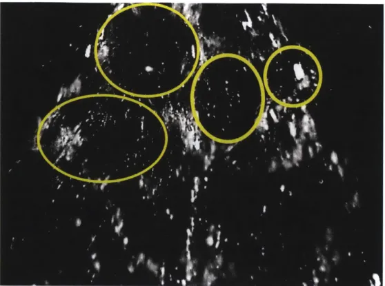
2-6 Top view of the multiple bag instability. Yellow ovals mark discrete, adjacent bags. . . . . 54

2-7 Regime diagram illustrating the observed dependence of the develop-ment of bags along a liquid jet in cross flow on the governing dimen-sionless groups. . . . . 54

(12)

2-9 Measured temporal bag diameters for a variety of experimental

condi-tion s. . . . . 57

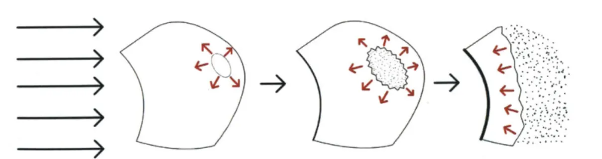
2-10 Schematic of the rupture and subsequent breakup of a bag. . . . . 57

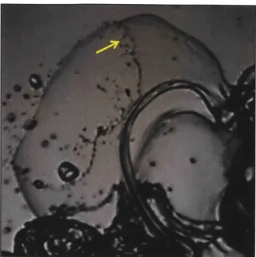
2-11 Ligaments are formed during bag membrane breakup and retraction. 58

2-12 Sequence showing the elongation of an upstream ligament with a thick-ened tip due to the downstream expansion of the bag and its rims. . . 58 2-13 Measured ligament dimensions at breakup for a variety of experimental

conditions. . . . . 59

2-14 Variation of upstream column wavelengths with WeG. Upstream col-umn waves for liquid jets in cross flow scale similarly with WeG theo-retically and experimentally for both single and multiple bag regimes. 61 2-15 Scaled temporal bag expansion diameter. This scaling holds true for

both single and multiple bags independent of WeG,

v

o, and q within

the bag breakup regime. . . . . 65 2-16 Temporal bag expansion diameter variability. Even for different

mea-surements from the same experiment, bag diameter values diverge at later times due to varying flow conditions that exist over time. . . 66

2-17 Overview of the instabilities that occur in the bag breakup regime.

RP signifies the Plateau instability, while RT is the Rayleigh-Taylor instability. . . . . 68 3-1 Simulated camera array in Blender. . . . . 80 3-2 Simulated images from each of the nine simulated cameras of a

chess-board calibration grid at particular orientation. . . . . 81 3-3 A three-dimensional plot of the relative locations of the grid points

from all of the simulated calibration images, including those shown in the previous figure. . . . . 81

3-4 Simulated raw images from each of the nine simulated cameras of a translucent sphere with a diameter of 5 mm. . . . . 82

(13)

3-5 Refocused images of the 5 mm diameter translucent sphere correspond-ing to the raw images in the previous figure. . . . . 82

3-6 Raw images from nine camera square array. . . . . 85

3-7 Sample calibration grid images for a particular grid orientation from

each of the nine cameras in the array. . . . . 86

3-8 Refocused images corresponding to the raw images shown in Figure 3-6. 86 3-9 Raw images from nine camera square array. . . . . 87 3-10 Refocused images corresponding to the raw images shown in the

pre-vious figure. . . . . 88

3-11 Raw images from nine camera square array. . . . . 89 3-12 Refocused images corresponding to the raw images shown in the

pre-vious figure. . . . . 90

4-1 Schematic of the evolution of a sheet into a jet and then droplets during atom ization. . . . . 96

4-2 Front view (top) and side view (bottom) of the destabilization of a

liquid sheet moving in air initially at rest. . . . . 98

4-3 Photograph of the atomization of a turbulent liquid sheet in air. . . . 99

4-4 Turbulent sheet of water flowing along an inclined plate; imaging was performed in the region where breakup and separation from the plate b egins. . . . . 102

4-5 Turbulent sheet experimental setup showing relative locations of the camera array for each experiment. . . . . 102

4-6 Ten camera array of Flea 2 model FL2-08S2M/C from Point Grey Research, Inc. CCD cameras, with 50mm Nikkor lenses, typical of

those used for the experiments presented herein. . . . . 103

4-7 Schematic of relative positions of the ten cameras in the array. . . . . 103

4-8 Sample calibration grid images for a particular grid orientation from

(14)

4-9 Sample refocused planes corresponding to the raw calibration grid im-ages shown in the previous figure. . . . 106 4-10 Raw array images at position 1, with the cameras focused on the sheet's

center. Here the flow rate is 278 gallons per minute. . . . . 107

4-11 Sample refocused planes corresponding to the raw calibration grid im-ages shown in the previous figure. . . . . 107

4-12 Raw array images at position 21, with the cameras focused on the sheet's center and rotated 30.8 clockwise from the horizontal to be aligned with the sheet. The liquid flow rate was 268 gallons per minute. 109 4-13 Two sample refocused planes with indicated in-focus features

corre-sponding to the raw images in the previous figure. . . . . 109

4-14 Raw array images at position 34, with the cameras focused on the near sheet edge and rotated 30.8 clockwise from the horizontal to be aligned with the sheet. The liquid flow rate was 270 gallons per minute 110 4-15 Two sample refocused planes with indicated in-focus features

corre-sponding to the raw images in the previous figure. . . . . 110

4-16 Raw array images at position 1, with the cameras focused on the near sheet edge and rotated 30.8' clockwise from the horizontal to be aligned

with the sheet. The liquid flow rate was 270 gallons per minute . . .111

4-17 Two sample refocused planes with indicated in-focus features corre-sponding to the raw images in the previous figure. . . . .111

5-1 Raw camera array images of ligaments and droplets in the spray re-sulting from a sneeze. . . . 118

5-2 Sample refocused image at plane z = _{24 mm. The in-focus node that}

is located at this plane is circled. . . . . 119 A-i Raw array images at position 1, with the cameras focused on the sheet's

center and rotated 30.8* clockwise from the horizontal to be aligned

(15)

A-2 Sample refocused planes with indicated in-focus features corresponding

to the raw images in the previous figure. . . . . 124

A-3 Raw array images at position 2, with the cameras focused on the sheet's

center and rotated 30.80 clockwise from the horizontal to be aligned

with the sheet. The liquid flow rate was 269 gallons per minute. . . . 125

A-4 Sample refocused planes with indicated in-focus features corresponding

to the raw images in the previous figure. . . . . 125

with the sheet. The liquid flow rate was 268 gallons per minute. . . . 126

center and rotated 30.8' clockwise from the horizontal to be aligned

(16)

A-14 Sample refocused planes with indicated in-focus features corresponding to the raw images in the previous figure. . . . . 130

A-19 Raw array images at position 10, with the cameras focused on the

sheet's center and rotated 30.80 clockwise from the horizontal to be aligned with the sheet. The liquid flow rate was 269 gallons per minute. 133

A-24 Sample refocused planes with indicated in-focus features corresponding

sheet's center and rotated 30.8* clockwise from the horizontal to be aligned with the sheet. The liquid flow rate was 269 gallons per minute. 136

(17)

sheet's center and rotated 30.80 clockwise from the horizontal to be

aligned with the sheet. The liquid flow rate was 269 gallons per minute. 137

sheet's center and rotated 30.8' clockwise from the horizontal to be aligned with the sheet. The liquid flow rate was 269 gallons per minute. 138

A-34 Sample refocused planes with indicated in-focus features corresponding to the raw images in the previous figure. . . . . 140

(18)

sheet's center and rotated 30.8 clockwise from the horizontal to be aligned with the sheet. The liquid flow rate was 268 gallons per minute. 143 A-40 Sample refocused planes with indicated in-focus features corresponding

to the raw images in the previous figure. . . . . 143 A-41 Raw array images at position 21, with the cameras focused on the

A-42 Sample refocused planes with indicated in-focus features corresponding to the raw images in the previous figure. . . . 144 A-43 Raw array images at position 22, with the cameras focused on the

to the raw images in the previous figure. . . . 145 A-45 Raw array images at position 23, with the cameras focused on the

to the raw images in the previous figure. . . . 146 A-47 Raw array images at position 24, with the cameras focused on the

A-48 Sample refocused planes with indicated in-focus features corresponding to the raw images in the previous figure. . . . 147 A-49 Raw array images at position 25, with the cameras focused on the

(19)

to the raw images in the previous figure . . . ... . . . . 148

A-54 Sample refocused planes with indicated in-focus features corresponding to the raw images in the previous figure. . . . . 150

sheet's center and rotated 30.8' clockwise from the horizontal to be

(20)

to the raw images in the previous figure. . . . 154

to the raw images in the previous figure. . . . 155

to the raw images in the previous figure. . . . . 158 A-71 Raw array images at position 36, with the cameras focused on the

to the raw images in the previous figure. . . . . 159 A-73 Raw array images at position 37, with the cameras focused on the

(21)

A-74 Sample refocused planes with indicated in-focus features corresponding to the raw images in the previous figure. . . . . 160 A-75 Raw array images at position 38, with the cameras focused on the

(22)

(23)

List of Tables

2.1 The parameter regime explored in this experimental study of a liquid

(24)

(25)

Chapter 1 Introduction

Sprays are a class of multiphase flows that result from the atomization of a volume of

liquid in the presence of a gas. Due to their prevalence and importance in both

na-ture and engineering applications, many experimental, computational and theoretical

investigations of sprays have been performed [2]. However, complete descriptions and

models of spray flows with even the simplest geometries continue to elude researchers

because of the complexity inherent in the study of sprays. They present a difficult

class of problems in fluid mechanics because of the complex interfacial physics that

come into play. All sprays include liquid and gas phases, and some may feature

solid particles as well. These flows are usually turbulent, making them difficult to

model. Thermal effects and evaporation also affect the evolution of sprays, further

convoluting the problem.

From an experimental viewpoint, it is difficult to quantitatively measure dynamic

spray characteristics. Imaging techniques are generally employed because pressure

probes and other invasive means would disrupt and modify the flow, especially in the

near-field region close to the jet or sheet nozzle exit, which is particularly difficult

to analyze. Throughout most sprays, the flow is optically dense, with ligaments and

droplets often occluding each other. This leads to considerable difficulty in effective

(26)

Figure 1-1: A high-speed photograph of a sprinkler at night by Edgerton (taken in 1939), recorded using a strobe fired for 10 ms [8].

employed suffer from a combination of issues ranging from complexity of the setup, to limited utility at the jet core, to only providing two-dimensional images, to overly

constraining the experimental setup in terms of optical access. These issues have

been overcome in the present study by employing a combination of the emerging

quantitative three-dimensional imaging techniques of light field imaging (LFI) and

synthetic aperture (SA) refocusing. By utilizing these methods, it is possible to

obtain a three-dimensional (3D) reconstruction of the spray flow and to "see through"

occlusions. Quantitative measurements of spray structures, such as droplets and

ligaments, may be extracted from these refocused volumes. (Traditional high-speed

imaging was also used to obtain time-resolved two-dimensional (2D) data.) This

information can be used to better understand sprays and to improve the design of

(27)

1.1 Spray Applications and Physics

1.1.1 Overview of Sprays

A sheet is formed when a fluid is injected into another relatively less dense fluid

through a narrow slit with a thickness significantly less than its width. If the slit

is circular, then a jet forms rather than a sheet. Sheet atomization actually occurs

much quicker than jet breakup [2]. The scale of the volume of liquid to be atomized

can range from light years in astronomical settings [3] to nanometers in a biological

context [4]. A thorough knowledge of the physics of atomization is important for

understanding the role of breakup behavior in many natural and engineering

appli-cations [6]. A book providing a review of the physics and applications related to

sprays and jets, including a summary of relevant experimental, computational, and

theoretical developments, has been published one year prior to this writing [2].

1.1.2 Spray Applications

Sprays play a pivotal role in many natural and engineering applications.

Break-ing ocean waves are an example of liquid sheet atomization in air. Waterfall mists

and rain are other forms of natural atomization [6]. Coughing and sneezing involve

sprays of droplets that can lead to airborne disease transmission [7]. Liquid atomizers

are found in diesel injectors, furnace burners, spray guns, spray driers, and sprinkle

chambers [2]. Figure 1-1 presents a high-speed photo by Harold Edgerton of water

jet atomization in a sprinkler [8]. The jets break up due to disturbances that are amplified by both capillary and inertial forces. Primary and secondary atomization

mechanisms that cause the breakup of the jets determine the resulting droplet size, position, and velocity distributions. These are important for understanding how to

(28)

maxi-mum efficiency.

Large industries, such as automotive, aerospace, and power-generation, that rely

on spray and droplet technologies involve annual production in the tens of billions of

dollars and possibly more [9]. Understanding the impact of design decisions on the

resulting spray droplet distributions and characteristics can lead to important

tech-nological improvements and lower costs. The design parameters that can generally

be controlled are injector size and shape, air speed, and liquid properties, such as

sur-face tension and viscosity [10]. It turns out that viscosity plays the most important

role of any liquid property in atomization [2]. Water and oil are the most common

liquids found in atomization processes, but non-Newtonian ("complex") fluids, such

as emulsions and slurries, as well as solid particles may be found in sprays as well, depending on the application [2].

Sometimes it is advantageous to stall atomization, while other applications

de-mand rapid breakup. Increasing the jet nozzle exit velocity and having the jet collide

with a solid object can hasten atomization [2]. Another technique that is used to

speed up atomization is the collision of jets, which atomize more quickly than do

single jets [2]. Figure 1-2 presents an example of a Rayleigh-Plateau instability (see

Section 1.1.3) found in the combustion chamber of the gas generator of an industrial

propulsion engine (this figure was taken from [11]). The sheets shown in this image

were formed by the collision of two liquid jets at an oblique angle. This type of

flow was first analyzed by Taylor [12] and Miller [13] in 1960 and has been further

investigated theoretically and experimentally by others [14, 15, 16, 17].

There are several types of jet atomizers. Figure 1-3 shows various types of

atomiz-ers organized by the type of energy that they employ along with schematics showing

general modes of operation (this chart was taken from [2]). The liquid itself provides

the kinetic energy to atomize it in pressure atomizers, including the jet, swirl, and

(29)

Figure 1-2: Impacting jets in the combustion chamber of the gas generator of an industrial propulsion engine, taken from [11].

are the most economical and widely used. Specifically, swirl atomizers are the most

popular. They involve the rotation of the liquid before it is emitted into the gaseous

environment.

Pneumatic atomizers feature the flow of the gaseous phase to help atomize the

liquid. The gas may flow parallel, perpendicular, or swirled around the liquid, which

enhances atomization by increasing the kinetic energy of the liquid and amplifying

instabilities that develop in the liquid volume (see Section 1.1.3). Flows of the kind

encountered in cross flow pneumatic atomizers will be analyzed in depth in Chapters

2 and 3. Rotary atomizers involve the transfer of kinetic energy from the rotating

device to the liquid, which breaks up to due centrifugal forces. A main disadvantage

of this type of atomizer is that high rotation speeds are necessary, which requires a

large power input. Other methods are also used, such as vibrating the apparatus to

hasten the atomization process. Often, a combination of atomizer types is employed.

In traditional atomizers, the efficiency of atomization, defined as the ratio of the

surface energy to the sum of surface energy, kinetic energy, and energy loss due to

(30)

efficient. However, the other more power-demanding methods are often required and

can be more effective

[2].

1.1.3 Spray Physics

Common Spray Instabilities

Thin jets or sheets of liquid are used in atomizers because these volumes have large

surface area and hence high surface energy, which leads to greater instabilities. In

most atomization processes, waves appear throughout the volume of liquid whose

am-plitudes quickly increase, leading to instabilities followed by breakup [2]. The state of

the gas of a spray plays an important role in the atomization process. For instance, critical and supercritical temperature and pressure are found in diesel engines [9].

Other critical parameters are the velocity of the gas, along with its density and

vis-cosity. These properties dictate the types of instabilities and, therefore, the physical

mechanisms governing the atomization process.

Rayleigh-Plateau Instability

Liquid jet atomization in an ambient gas has been examined quantitatively since

the 19th century [2, 18]. Plateau found that a liquid jet in still air breaks into spherical droplets to minimize surface tension. This is the phenomenon that is responsible, for

instance, for the breakup of a liquid column from a faucet into droplets (Figure 1-4).

Plateau stated that a jet breaks up into segments of equal length, each of which has a length of 27r times the jet radius [19]. Droplets then form from these sections of

the jet due to surface tension. It could be considered ironic that the cohesive force of

surface tension actually ends up causing the atomization of jets into ligaments and

(31)

Figure 1-3: Classification of atomizers, taken from [2].

(32)

it is more energetically favorable for the liquid column to take the form of discrete droplets as opposed to remaining as a continuous jet. It turns out that the surface area of the resulting droplets is less than that of the original liquid jet when the final droplet radius exceeds 1.5 times the jet radius [21].

Rayleigh showed that hydrodynamic instability is the cause of jet breakup in this case [22, 23]. A linear stability analysis involving perturbing the radius, surface veloc-ities, and pressure distribution on a column of liquid in the equilibrium state shows that the disturbance wavelength along the jet for the fastest growth rate of instability is about 9.02 times the undisturbed jet radius, or 143.7% of its circumference. These results were found by neglecting the ambient fluid, viscosity of the liquid jet, and gravity. Rayleigh also showed that for a viscous jet in an inviscid gas (neglecting the mass of the gas), the most unstable wavelength is infinitely long [24]. For an inviscid gas jet in an inviscid liquid, the most unstable wavelength was found to be 206.5% of the undisturbed jet circumference [25].

Tomotika found that there is a ratio of the viscosities of the jet and ambient gas that maximizes the growth rate of jet instability [26]. Unlike Rayleigh, Chandrasekhar included the liquid viscosity and density in his model of jet breakup and demonstrated theoretically that viscosity slows down atomization and increases the resulting drop diameter [22]. The experimental investigations of Donnelly and Glaberson [28] as well as Goedde and Yuen [29] agree with the theory developed by Rayleigh and Chandrasekhar.

Rayleigh-Taylor Instability

The Rayleigh-Taylor instability occurs when a fluid of less density, such as air, is accelerated towards one of greater density, e.g. water [22]. This type of instability can occur when a heavier fluid is located above a lighter fluid. In the context of sprays, it

(33)

K d

-|f>

Figure 1-4: Rayleigh-Plateau instability.

is relevant in pneumatic atomizers involving a liquid jet in a cross flow of air. The air moves toward the relatively heavier fluid and bends the liquid jet in the downstream direction due to the aerodynamic drag force. As the air flows along the curved jet, it accelerates, creating waves along the jet surface. Figure 1-5 presents a schematic of the development of the Rayleigh-Taylor instability in a liquid jet in cross flow. UG is the gas velocity, V is the liquid nozzle exit velocity, dj is the nozzle exit diameter,

dl is the length of the segment of the jet, and R is the radius of curvature of the

deformed jet. Ac is the most unstable wavelength for the Rayleigh-Taylor instability, which is 2v/57r(o/(pac))1/2

(neglecting viscosity), where o- is the surface tension, p is the liquid density, and ac is the acceleration [22].

Kelvin-Helmholtz Instability

In most atomization processes, the liquid volume often becomes a sheet, at least

0

(34)

dl

_UG

die

R

UG

c F --Fiue15:Ryeg -Talrisaiiy

(35)

in intermediate breakup stages [9]. The next stage of atomization is primary breakup, during which ligaments are formed. These structures then shatter into droplets and determine the final droplet size distribution in the spray [31]. The level of corrugation of ligaments and other structures at the time of breakup is also important in setting droplet size distribution [32]. A liquid sheet in the presence of an ambient gas will develop waves naturally when moving fast enough relative to the gas due to a shear, Kelvin-Helmholtz type instability [33, 34] that exacerbates any disturbances in the

sheet [6, 12, 9]. .This type of instability is caused by the relative (parallel) motion

between two adjacent fluids of different densities (or of different layers of a single

density stratified fluid).

Figure 1-6 shows a schematic of the destabilization of a plane liquid sheet of

thickness h in air at rest [6, 12, 9]. The sheet is moving to the right with a velocity u and is perturbed by a disturbance with amplitude ( and phase

#.

p, pa, and r

are the liquid density, gas density, and distance along the sheet, respectively. For

two fluids arranged horizontally moving parallel to each other with different densities

(neglecting surface tension), the maximum unstable wavelength due to the Kelvin-Helholz nstbiityis21ra1Ce2(U1 -U2 )2

Helmholtz instability is 9* , 'where ai and a2 are the ratios of the density of

each fluid to the sum of the densities, g is the acceleration due to gravity, and U1 and

U2 are the constant velocities of each of the fluids, respectively [22]. This instability

will be discussed in greater depth as it applies to the breakup of a turbulent water

sheet in air in Chapter 4.

1.2 Light Field Imaging

A fundamental challenge in experimental fluid mechanics is the accurate spatial and

temporal resolution of three-dimensional, multiphase fluid flows, such as sprays.

(36)

bench-Z

-h/2-Figure 1-6: Destabilization of a plane liquid sheet of thickness h in air at rest, taken from [9].

marking computational codes, fully spatially- and time-resolved experimental data is

paramount. Given recent advances in camera and imaging technologies, and the

grow-ing prevalence of commercially available light field imaggrow-ing systems, the opportunities

for obtaining such data are achievable at a lower cost and with greater resolution and

computational savings. Stemming from the computer vision communities, light field

imaging (LFI) and synthetic aperture (SA) refocusing techniques have been combined

in an emerging method to resolve three-dimensional flow fields over time [1]. This

technique is aptly suited for sprays, particle laden and multiphase flows, as well as

complex unsteady and turbulent flows.

At the core of light field imaging, a large number of light rays from a scene are

collected and subsequently reparameterized based on calibration to determine a 3D

image [2]. In practice, one method used by researchers in the imaging community for

sampling a large number of rays is to use a camera array [37, 38] or more recently, a single imaging sensor and a small array of lenslets (lenslet array) in a plenoptic

camera (e.g. [5]). The combined LFI and SA approach is applied herein to the

reparameterization methods to 3D spray fields and fluid flows.

In short, light field imaging involves the reparameterization of images captured

(37)

camera), to digitally refocus a flow field post-capture. All cameras record a volumetric

scene in-focus, and by recombining images in a specific manner, individual focal

planes can be isolated in software to form refocused images. Flow features, such as individual droplets, can be located in 3D by refocusing throughout the volume and

extracting features on each plane. An implication of the refocusing is the ability to "see through" partial occlusions in the scene. This method extends measurement capabilities in complicated flows where knowledge is incomplete. Utilization of this

technique allows for finer measurements of flow quantities and structures that would

have been impossible with prior methods.

In particular, this imaging system is designed to measure and locate features, such as bubbles, droplets and particles in three spatial dimensions over time in multiphase

flows. Other measurement systems often only allow practitioners to measure aver-age quantities or envelopes of flow regions that do not require such high resolution.

This new technique has already demonstrated the capability to resolve very fine flow

features, which is especially important in multiphase and turbulent flow fields that

contain very minute flow structures and length scales. An instrument of this kind is of

great aid in a variety of engineering applications in areas such as air-sea interaction, naval hydrodynamics, aerospace, turbulence and beyond.

1.3 Outline of Thesis

Chapter 2 presents a theoretical and experimental investigation of a liquid jet in

gaseous cross flow in the bag breakup regime. Bags are partial bubbles that form

along the jet due to the aerodynamic drag force of the air on the liquid jet. Water

jets emanating vertically downward into a horizontal wind tunnel were recorded using

traditional 2D high-speed video to analyze the instabilities that develop in the jet as well as primary and secondary jet breakup. It was discovered that there is a

(38)

transition regime from single to multiple side-by-side bags for liquid jet diameters that are approximately equal to the liquid's capillary length (which is approximately

2.7 mm for water). Once this diameter size is exceeded, multiple bags are consistently

present throughout the length of the liquid jet in a gaseous cross flow in the bag breakup regime.

Chapter 3 discusses further development and validation of the light field imaging and synthetic aperture refocusing techniques. These methods are then applied to the liquid jet in cross flow experiments described in Chapter 2. These 3D imaging techniques were used to reconstruct an image volume from the images taken by each of the individual cameras in the arrays used to image the flows.

In Chapter 4, an experimental investigation of the atomization of a turbulent sheet of water launched into the air at an angle is presented. As in Chapter 3, light field imaging and synthetic aperture refocusing techniques are utilized to analyze this flow. The focus here is the primary sheet breakup into ligaments and relatively large droplets on the underside of the sheet. These flow features were successfully resolved in three dimensions.

Finally, Chapter 5 presents conclusions for the entire thesis. A summary of the physical insights gained into the various sprays that were analyzed is provided. In addition, the synthetic aperture imaging results are summarized. Applications of the combined LFI and SA methods to other flows, such as sneezing and airborne disease transmission, are discussed. Future steps to be taken are outlined.

(39)

Bibliography

[1] N. Ashgriz. Handbook of Atomization and Sprays: Theory and Applications.

New York, NY: Springer. 2011.

[2] L. Bayvel and Z. Orzechowski. Liquid Atomization. Washington, DC: Taylor & Francis. 1993.

[3]

P. A. Hughes. Beams and Jets in Astrophysics. Cambridge University Press.

1991.

[4] S. Benita. Microencapsulation. Marcel Dekker. 1996.

[5] S. P. Lin. Breakup of Liquid Sheets and Jets. Cambridge University Press. 2003. [6] A. H. Lefebvre. Atomization and Sprays. New York: Hemisphere. 1989.

[7] J. K. Gupta, C.-H. Lin, and

Q.

Chen. Flow dynamics and characterization of a cough. Indoor Air, 19(6):517-525. 2009.

[8] H. E. Edgerton, E. Jussim, and G. Kayafas. Stopping time: the photographs of

Harold Edgerton. New York: H. N. Abrams. 1987.

[9] W. A. Sirignano. Fluid Dynamics and Transport of Droplets and Sprays.

Cam-bridge, UK: Cambridge University Press. 1999.

[10] E. Villermaux. Fragmentation. Annual Review of Fluid Mechanics, 39(1):

419-446. 2007.

[11] N. Bremond and E. Villermaux. Atomization by jet impact. J. Fluid Mech., 549: 273-306. 2006.

(40)

[12] G. I. Taylor. Formation of thin flat sheets of water. Proc. R. Soc. Lond. A, 259:

1-17. 1960.

[13] K. D. Miller. Distribution of spray from impinging liquid jets. J. Phys 31: 1132-1133. 1960.

[14] M. F. Heidmann, R. J. Priem, and J. C. Humphrey. A study of sprays formed

by two impacting jets. NACA IN 3835. 1957.

[15] N. Dombrowski and P. C. Hooper. A study of the sprays formed by impinging

jets in laminar and turbulent flow. J. Fluid Mech. 18: 392-400. 1963.

[16] E. A. Ibrahim and A. Przekwas. Impinging jets atomization. Phys. Fluids A 3: 2981-2987. 1991.

[17] J. W. M. Bush and A. E. Hasha. On the collision of laminar jets: fluid chains

and fishbones. J. Fluid Mech. 511: 285-310. 2004.

[18] S. P. Lin and R. D. Reitz. Drop and Spray Formation from a Liquid Jet. Annual

Review of Fluid Mechanics, 30: 85-105. 1998.

[19] J. Plateau. Statique Experimentale et Theorique des Liquids Soumis aux Seules

Forces Moleculaire. Paris: Cauthier Villars. 1, 2: 450-495. 1873.

[20] J. Eggers and E. Villermaux. Physics of liquid jets. Rep. Prog. Phys. 71: 036601.

2008.

[21] P.-G. de Gennes, F. Brochard-Wyart, and D. Quer6. Capillarity and Wetting Phenomena: Drops, Bubbles, Pears, Waves. New York, NY: Springer. 2004. [22] Lord Rayleigh. On the capillary phenomenon of jets. Proc. R. Soc. London. 29:

71-97. 1879a.

[23] Lord Rayeligh. On the instability of jets. Proc. Lond. Math. Soc. 10: 4-13. 1879b.

[24] Lord Rayleigh. On the instability of a cylinder of viscous liquid under capillary force. Phil. Mag. 34:145-54. 1892a.

(41)

[25] Lord Rayleigh. On the instability of cylindrical fluid surfaces. Phil. Mag. 34:177-180. 1892b.

[26] S. Tomotika. On the instability of a cylindrical thread of a viscous liquid

sur-rounded by another viscous fluid. Proc. R. Soc. London Ser. A. 150:322-37. 1935.

[27] S. Chandrasekhar. Hydrodynamic and Hydromagnetic Stability. Oxford: Oxford

Univ. Press. 1961.

[28] R. J. Donnelly and W. Glaberson. Experiments on the capillary instability of a

liquid jet. Proc. R. Soc. London Ser. A. 290:547.-56. 1996.

[29] E. F. Goedde and M. C. Yuen. Experiments on liquid jet instability. J. Fluid

Mech. 40:495- 512. 1970.

[30] N. Bremond, C. Clanet, and E. Villermaux. Atomization of undulating liquid

sheets. J. Fluid Mech. 585: 421-456. 2007.

[31] F. Savart. Memoire sur la constitution des veines liquides lances par des orifices

circulaires en mince paroi. Ann. de chim. 53: 337-398. 1833a.

[32] E. Villermaux, P. Marmottant, J. Duplat. Ligament-mediated spray formation.

Phys. Rev. Let. 92: 074501. 2004.

[33] H. von Helmholtz. On discontinuous movements of fluids. Phil. Mag. 36: 337-346. 1868.

[34] Lord Kelvin. Hydrokinetic solutions and observations. Philo. Mag. 42: 362-377.

1871.

[35] J. Belden, T. T. Truscott, M. Axiak, and A. H. Techet. Three-dimensional

syn-thetic aperture particle image velocimetry. Meas Sci Technol 21:1-21. 2010.

[36] A. Isaksen, L. McMillan, and S. J. Gortler. Dynamically reparameterized light

field SIGGRAPH '00: Proc. 27th Ann. Conf. on Computer Graphics and Inter-active Techniques (New York: ACM Press/Addison-Wesley). 297-306. 2000.

(42)

[37] V. Vaish, B. Wilburn, N. Joshi, and M. Levoy. Using plane + parallax for cali-brating dense camera arrays Proc. 2004 IEEE Computer Society Conf. on Com-puter Vision and Pattern Recognition (CVPR04') (June-July 2004) v. 1, Los

Alamitos, CA: IEEE Computer Society Press. 2-9. 2004.

[38] V. Vaish, G. Garg, E. Talvala, E. Antunez, B. Wilburn, M. Horowitz, and M.

Levoy. Synthetic aperture focusing using a shear-warp factorization of the

view-ing transform. Proc. IEEE Computer Society Conf on Computer Vision and

Pattern Recognition (CVPR05')-June Workshops. Los Alamitos, CA: IEEE Computer Society Press 3:129. 2005.

[39] K. Lynch. Development of a 3-D Fluid Velocimetry Technique based on Light

(43)

Chapter 2 Hydrodynamic Instabilities in

Round Liquid Jets in Gaseous

Cross Flow

Water jets in the presence of uniform perpendicular air cross flow were investigated theoretically and experimentally using high-speed imaging for gaseous Weber number

WeG PGUGd/o- (where PG is the density of the gas, UG is the velocity of the gas,

dj is the liquid jet nozzle exit diameter, and o is the surface tension) below 30,

small liquid jet Ohnesorge number Oh = j/ p/jvo-dj (where pj is the density of the

liquid and pj is the liquid's viscosity), and large Reynolds numbers for the liquid

Rej = pjVjdj/p (where Vj is the liquid jet nozzle exit speed) and gas ReG =

PGUGdJ/pG (where pG is the gaseous phase's viscosity). Previously, a bag instability

has been reported for 4 < WeG < 30. Jets first deform into curved sheets due to

aerodynamic drag, followed by the formation of partial bubbles (bags) along the jet streamwise direction that expand and ultimately burst. Single bags were present at each streamwise position along the liquid jets in prior experiments featuring liquid jet nozzle diameters less than the capillary length of water. It has been found that at larger nozzle diameters it is possible to observe multiple bags at the same streamwise

(44)

jet position because single bags of such large sizes would be unstable. Measurements of bag expansion diameters over time for a wide range of experimental conditions were found to follow the trend predicted by a theoretical analysis. A theoretical derivation for the upstream jet column wavelength was found to match experimental data in both the single and multiple bag regimes. Other flow features, such as upstream ligament extension properties, were measured and analyzed as well.

2.1 Introduction

The formation and subsequent breakup of bag-like bubble structures emanating from round nonturbulent liquid jets in uniform gaseous cross flow within the bag breakup regime were studied experimentally and theoretically. Atomization of liquid jets and sheets has numerous significant applications, including film coating, nuclear safety curtain formation, agricultural sprays, ink jet printing, fiber and sheet drawing,

pow-der metallurgy, toxic material removal, encapsulation of biomedical materials, and

spray combustion. While some applications require more rapid jet breakup rates, in other cases it is desirable to reduce the speed of atomization, making knowledge of the

mechanism of jet atomization critical

[1].

Spray flows with very rapid cross flow air speeds are applicable to combustion in air-breathing propulsion systems, such as gas turbine augmentor systems [2]. [3] examined the role of surface tension in jet instabil-ity. [4] analyzed jet stability with acoustic excitation of the jet. The Rayleigh-Plateau instability is responsible for the capillary breakup of a liquid jet, such as a column of liquid from a faucet. [1],

[5],

and [6] review many other investigations related to liquid jets flowing under a wide variety of conditions.

Some prior studies of round nonturbulent liquid jets in uniform gaseous cross flow investigated depth of penetration of the liquid jet and jet trajectories for various

(45)

in liquid jets accompanied by a coaxial flow of gas [11] and in drop deformation

and breakup in a flow of air. The most relevant studies to the present investigation

are

[8,

12, 13, 15].

[12]

developed a regime map for liquid jets in cross flow based

on WeG and the momentum flux ratio q = pjVJ/(pGUG). WeG is a dimensionless

parameter that indicates the relative importance of the inertia of the gas and surface tension, while q is the ratio of the liquid's inertia to that of the gas. Mazallon

et al. found that for Oh < 0.1, the regimes are only governed by WeG. They

also created a new regime map with Oh and WeG as the coordinates, which [8]

modified later. When viscous effects are small (Oh < 0.1),

[13]

found that breakup regime transitions of the liquid jet are determined by WeG number as follows: column

breakup (WeG < 4), bag breakup (4 < WeG < 30) (modified by [8]), multimode

breakup (30 < WeG < 110), and shear breakup (WeG > 110). Figure 2-1 presents

a regime diagram with photographic examples of each known instability category

(adapted from [8]). The bag breakup regime is highlighted because it is the focus of

the present study. [15] recently published an article about the bag breakup regime of

liquid jets in cross flow. It discusses many statistics about the formation of nodes on

bags and breakup of bags into tiny droplets due to the breakup of the bag membrane, larger droplets caused by the atomization of the two strings of the ring bounding

the base of the bag, and still larger droplets associated with bag nodes. The size of

bag droplets is independent of WeG, but node- and ring-droplet sizes decrease with

increasing WeG. Column waves are also described mathematically in light of the

Rayleigh-Taylor instability, which occurs when a fluid is accelerated towards another

relatively heavier fluid [4].

The present study explores the destabilization and primary breakup mechanisms

of a liquid jet in cross flow. §2.2 describes the experimental methods employed in

this study and §2.3 presents the results of the experimental investigation. A new

(46)

We*=0 We=3 We%=8 We,= 30 We=l 220

Figure 2-1: Liquid jet in cross flow breakup regimes based on We0 (adapted

from [8]).

at the same streamwise jet position when the jet nozzle diameter exceeds the capillary

length. It was also found that a regime exists when the jet nozzle diameter equals

the capillary length that marks a transition between the single and multiple bag

regimes. Various flow measurements are made in the single bag, multiple bag, and

transition regimes. In §2.4 equations are developed to describe the upstream column

wavelength and bag expansion diameter over time. Experimental data are found to

match the trends predicted by these formulas. Finally, the instabilities responsible

for the primary breakup mechanisms of a liquid jet in cross flow are detailed in §2.5.

2.2 Experiments

This experimental study is composed of three parts. The first is an exploratory

investigation of the flow structures generated in the case of a liquid jet in gaseous

cross flow. Secondly, a careful quantitative study of the upstream column waves is

performed and the instability responsible for them investigated. Finally, the formation

and destruction of fluid bags are studied experimentally in order to test the validity of

(47)

jet ligament dynamics.

A schematic illustration of the apparatus used in this experimental study is

pre-sented in Figure 2-2. Water was injected downward into a horizontal wind tunnel

to generate the multiphase flows under consideration. The wind tunnel test section

width, height, and length were 1, 1, and 2.5 ft, respectively. The water was pumped

from the reservoir through polystyrene tubing into metal water jet nozzles of

di-ameters in the range of 1-9 mm. Water volume flow rates were controlled using a

variable-flow pump (Cole Parmer, Model EW-75211-60) and were measured with a

digital flowmeter (AW Company Model JFC-01) that gave an accuracy of 0.1% over

the range considered. The speed of the water exiting the nozzle was measured by

collecting a measured volume of water over a specified amount of time. Streamwise

velocity measurements were made via image analysis using MATLAB code in a

man-ner similar to that described in

[15].

As has been previously noted and confirmed in the present study, the instantaneous speed at any streamwise point along the jet

is essentially the same as the nozzle exit velocity

[15].

An anemometer was used to measure the air cross flow speed (La Crosse Technology, Model EA-3010U) with an

accuracy of 0.1 m/s. Characteristic flow rates and other experimental parameters are

listed in Table 2.1. Images were acquired using an IDT X-Stream XS3 high-speed

camera with a Nikon Nikkor 28 mm lens. Most of the images were recorded from a

side view, but angled top views were recorded as well to better understand the flow

structures. All images were recorded at 1630 frames per second. Two IDT 19-LED

pulsed light banks were synchronized with the camera to back light the flow being

Analysis of multiphase fluid flows via high speed and synthetic aperture three dimensional imaging

OCT 2 2 2012

RI

RIES

Analysis of Multiphase Fluid Flows via High Speed and

Synthetic Aperture Three Dimensional Imaging

by

Barry Ethan Scharfman

Abstract

Acknowledgments

Contents

List of Figures

v

List of Tables

Chapter 1

Introduction

1.1

Spray Applications and Physics

[2].

1.1.3

Spray Physics

K d

-|f>

0

0

dl

UG

R

UG

UG

#.

1.2

Light Field Imaging

1.3

Outline of Thesis

Bibliography

[3]

Q.

Chapter 2

Hydrodynamic Instabilities in

Round Liquid Jets in Gaseous

Cross Flow

2.1

Introduction

[1].

[5],

[8,

[12]

[13]

2.2

Experiments

[15].

[15].

_UG