Calculations of radiation opacity for high Z elements

Calculations of radiation opacity for high Z elements

By TOMASZ BLENSKI AND JACQUES LIGOU

Institute de Genie Atomique, Departement de Physique,

Ecole Polytechnique Federate de Lausanne, CH-1015 Lausanne (Switzerland) (Received 13 December 1988)

We present some results of our opacity calculations for lead and gold at temperatures and densities relevant to ICF conditions. We use an average atom model based on the temperature dependent Thomas-Fermi shell approach. The absorption bands (broaden-ing of lines) are accounted for with a simple T.F. fluctuation formula. The independent particle bound-bound, bound-free, and free-free photon cross-sections are taken without further approximations.

1. Introduction

Radiative opacities are important physical data in simulations of inertial-confinement-fusion (ICF) and in astrophysics. In ICF calculations the radiative transfer is usually taken into account in the diffusion approximation (Long & Tahir 1987). The parameter which is then needed is the Rosseland mean opacity. Moreover, the validity of the diffusion ap-proximation depends in turn on the values of opacities. The knowledge of opacities for all relevant temperatures and densities and as a function of photon frequency is therefore required in order to correctly model the transport of photons in the ICF pellets.

In the astrophysical literature the elements of interest have Z (atomic number) less than or equal to 26 (iron) (Carson et al. 1968; Cox 1965). In ICF calculations especially impor-tant are opacities of high Z elements like gold (Nardi & Zinamon 1979) or lead (Long & Tahir 1987) which are used as pellet tampers. There are quite a few papers treating some cases of opacities for astrophysical applications but the opacities of high Z elements are rare in the published literature. Some reasons which explain this situation were given in Armstrong and Nicholls (1972). Concerning the published high Z opacities, we can mention here the work of Nardi & Zinamon (1979). In the papers of Pritzker et al. (1975a, 1975b), the atomic model is the hydrogenic one, and the bound-bound transitions are neglected in the photon cross section, and it is a serious drawback since these (bb) transi-tions have been recognized as giving dominant contribution to opacities in the case of high Z (see Nardi & Zinamon (1979) and this paper).

In the paper of Nardi and Zinamon (1979) the atomic model is much more involved, and a special procedure is applied in order to account for the degree of ionization and the formation of absorption bands. The element of interest is gold at a temperature of 750 eV and at solid density. First, the Saha equation is solved which yields first estimates for ion fractions with different charge states. For each ion type the electron energy levels and wave functions are found with a zero temperature Thomas-Fermi (T.F.) model. The charge distribution is then recalculated from a partition function containing the energy levels. For each ion, the photon cross-sections bound-bound (bb), bound-free (bf), and free-free (ff) are obtained using single electron matrix element formulas for (bb) and sim-plified Kramers type expressions for (bf) and (ff). The plasma effects are included by lowering the ionization potentials of (bf) and in the Moszkowski-Meyerott formula of

266 T. Bteriski and J. Ligou

line broadening (Cox 1965) which contains plasma electron density. The creation of ab-sorption bands, which is a typical feature of high temperature and density matter, results in the paper of Nardi and Zinamon (1979) from two effects: the first is the splitting of lines into multiples with electron impact line broadening, the second is the presence of different ion types, the corresponding energy levels of which are shifted one with respect to others.

In the present paper the atomic physics model will be different. We will use the temperature-dependent T.F. model of Latter (1955), which accounts also for finite den-sity (Appendix A). All the existing bound energy levels of the T.F. potential will be found by solving the Schrodinger equation with a modified shooting method (Bteriski & Ligou 1988a). In order to calculate the cross sections involving (bf) and (ff) matrix elements (Appendix B) the continuous spectrum wave functions will be calculated when needed. The populations of both the bound and free states will be found according to the Fermi-Dirac statistics with the chemical potential of the T.F. model. In order to account for the finite line widths and absorption bands we will follow the density functional theory of fluctuations of electron density in the T.F. model (Bteriski & Cichocki 1988), the same as used for electronic states. We will assume, however, as in the work of Shalitin et al. (1984) that the fluctuations of energy levels are independent. From the numerical point of view our approach to absorption bands presents no more problems than the calcula-tion of the (bb) matrix elements themselves.

From the physical point of view our approach seems to be the simplest possible, and can take into account finite temperature and density, and all (bb), (bf) and (ff) transi-tions. We do not consider plasma effects (Nardi & Zinamon 1979). Our model is selfcon-sistent only in the sense of the T.F. theory and we neglect exchange and correlation potentials as well as relativistic effects. These problems will be addressed in a future study. We will use, however, full expressions for the cross-sections (Appendix B) and always include in our calculations all the existing bound states, the number of which may be large, especially for small densities and high temperatures. Our aim is to obtain some preliminary data concerning opacities of gold and lead in the physical conditions relevant to ICF and to recognize crucial points in the numerical procedures. We hope that with the present model we can get some idea of how sensitive opacities are to changes of tem-perature T and density p and what the importance is of (bb), (bf) and (ff) transitions in different domain of p and T with Z of the order of 70-90.

2. Rosseland (K

) mean opacity

The derivation of mean Rosseland opacity and the discussion about its validity range may be found elsewhere (Armstrong & Nicholls 1972; Pomraning 1973), see also (Carson

et al. 1968; Cox 1965; Nardi & Zinamon 1979). Here we only give the final formula:

</w4exp( y

(1)

r\f) ~

where T is temperature, v frequency, h Planck constant and

with /?,-, i = 1,... I; being atomic densities of each element of the medium, p is the total mass density, while the total cross-section includes the stimulated emission according to:

asJ(p); (3)

where afl>, and aSii are the absorption and scattering cross-sections respectively, of i-th

element. We have finally (see for instance Armstrong & Nicholls 1972; Bleriski & Ligou 1988b)

bb bf ff

Oa.M = °a,M + Ga,i(v) + <V(") • (4)

The full expressions of (bb), (bf) and (ff) cross-sections are given in Appendix B. In the numerical examples of this paper we only consider one element media. An extension to mixture is straightforward. The scattering cross-section is taken as a constant, equal to the Thomson cross-section multiplied by Z. We found, as it was suggested earlier (Nardi & Zinamon 1979), that this term was nearly negligible.

3. Numerical methods

From the formulas cited in Appendix B and the form of equations (1) and (2) it is easy to guess that a numerical evaluation of opacities is a rather formidable task. This is espe-cially true in the case of the Rosseland value since the calculation of the harmonic mean is more sensitive to the behavior of the section. Among the (bb), (bf) and (ff) cross-sections of Appendix B the most troublesome seems to be the last one (equation B4) since it requires, for a given frequency v, two integrations and one infinite summation upon the angular quantum numbers la. It is only partially true since this cross-section behaves

rather regularly, nearly as l/v3. For this reason the (ff) cross-section has been often taken

in the classical Kramers approximation (Carson et al. 1968). This approximation has been compared with the formula of equation B4 and it was found that the Gaunt factor, which accounts for accuracy of Kramers formula, could be in some extreme cases even of the order of 10 (Weber 1988). We decided therefore to use equation B4 without further ap-proximations. The contribution of (ff) transitions to the opacities considered in the pres-ent paper is rather small as we show later on. We preferred however to implempres-ent in our codes a rather accurate (ff) cross-section module for future calculations of highly ionized or intermediate Z elements. Since the calculation of (ff) cross-section is expensive from the point of view of the CPU time, we decided to use the following interpolation scheme:

aIf(v) = a0 + fl, - + a2 — + «3 —; (5)

V V V

and to perform actual evaluation of af/(v) only in a given number of points. The

coef-ficients ah i = 0,1,2,3, are obtained locally from the set of four linear equations as in

the spline method.

For the calculations of (bb) and (bf) cross-sections one needs all bound energy levels, all bound and many free wave functions calculated with sufficient accuracy. In our code the bound states are found with the method of Blenski & Ligou (1988a) based on a Nou-merov finite difference scheme. A common spatial mesh with variable steps (see Herman & Skillman (1963)) is used in order to account for strong gradients of wave functions near the origin. The same Noumerov finite difference scheme and mesh are used in the

268 T. Bteriski and J. Ligou

case of the free electron wave functions. Since the number of existing bound states is not known a priori, the vectors of the bound wave functions are not declared but, in-stead, are stored on a file and read when necessary. The routine for free electron wave function is always called locally and the corresponding vectors are not stored. The CPU time of this routine is however not negligible and for this reason an interpolation tech-nique, equation 5, has been applied to (bf) cross-section (equation B3). An additional problem appears here since the (bf) cross-section has singular behavior in v (the photeffect edges) and its spline interpolation should always be expanded on frequency points lying between two neighboring edges. These points are therefore found automatically during execution of the program.

The (bb) cross-section (equation B2) does not require any interpolation technique since for each frequency v only the calculation of line shape functions/ot (v — vab) (equation

C12, Appendix C) is needed. All other elements of the formula B2 (the matrix elements and the half widths) are stored once for all.

Our results, which we present and discuss in the next section, concern the mean opaci-ties (averaged over the whole frequency range), but our code produces, as well, multi-group opacities (Pomraning 1973). All integrations over the frequency in the final formulas for the opacities (for the total opacities the corresponding equations are equations 1-2) are performed independently with Gauss and Kronrod quadrature routines. The group frequency regions are subdivided into "fine" integration intervals in such a way that no interval contains any of the (bf) edges. Moreover, each (bb) line (equation B2) has its own "fine" interval. Inside each interval we use 41 points Kronrod and 20 points Gauss routines. Finally, in order to get multigroup or total opacities, the results of "fine" inte-grations are added up. The "fine" integration structure is found by the code and depends, of course, upon the details of the atomic spectrum. The difference between two values of opacities which are obtained with the Kronrod and Gauss quadratures are considered as a measure of integration accuracy.

Various tests have been performed to control the accuracy of the calculations of the energy levels and both bound and free wave functions. The most important of them are oscillator strength sum rules (Bethe & Salpeter 1957) (Appendix D).

4. Some results and conclusions

The results, produced by the code described above, are presented in five tables. We concentrate on two elements important for ICF: "gold" (Z = 79) and "lead" (Z = 82). We prefer to use inverted commas to indicate that our model is rather simple.

These calculations have been performed for four values of temperature (100 eV, 316.2 eV, 750 eV, and 1000 eV) and three values of density (po, that of the solid, po/5,

and po/l0. The solid density of lead was taken as 11.34 g/cm3 and that of gold as 19.34

g/cm3.

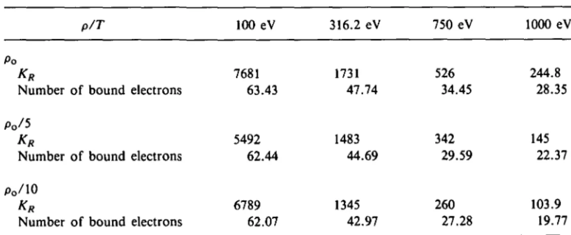
In table 1 we show Rosseland opacities in crnVg and mean numbers of bound elec-trons defined as follows (Rozsnyai 1972):

f IE , - n\ "h1

Nb= £ 2(21 + 1) exp - ^ + 1 (6)

n.i L \ ^ / J

with a being the T.F. chemical potential (equation A16). Although the model is not self-consistent, the differences between the number of bound electrons given by the T.F. semi-classical expression NbF-, and Nb from equation 6 are not large. For instance in the case

TABLE 1. Rosseland opacities (in cm2/g) and numbers of bound electrons of gold Po Number Po/5 KR Number Po/10 KR Number p/T of bound of bound of bound electrons electrons electrons 100 eV 7681 63.43 5492 62.44 6789 62.07 316.2 eV 1731 47.74 1483 44.69 1345 42.97 750 eV 526 34.45 342 29.59 260 27.28 1000 eV 244.8 28.35 145 22.37 103.9 19.77 NjF- = 33.88, Nb = 34.45.

Gold at this temperature and density has been considered by Nardi and Zinamon (1979). They obtained 35 as the most probable charge state (fraction 0.22 of the total ion popula-tion) accompanied by 34 (fraction 0.20) and 36 (fraction 0.15).

The Rosseland value in Nardi and Zinamon (1979) is given in terms of mean free path. Inverting to opacity, one gets for their total opacity (i.e. with (bb) transitions included):

jf Total = 4 3 1 8 c m2/ g >

while for the opacity without (bb):

Kg*" = 148 cmVg.

Our result (table 1) is:

K]total = 525 cmVg.

Following Nardi and Zinamon we illustrate in tables 2-4 the importance of (bb), (bf) and (ff) processes for the values of opacities. For the above cited case of Nardi and Zina-mon (1979) we find in table 3 the Rosseland opacity without (bb) and (ff):

which leads to the same conclusion about the dominant contribution of the (bb) transitions. This dominant contribution of (bb) has been confirmed for all temperatures and

densi-P/T Po Po/5 Po/10 TABLE 2. KR KR KR

Opacities of gold (in 100 eV 5795 5019 6464 cm2/g) with 316.2 eV 1646 1459 1332 <jff(i') neglected 750 eV 512 336 255 1000 eV 238.7 142 101.8

270 T. Bteriski and J. Ligou

TABLE 3. Opacities of gold (in cm2/g) with a(t(") and abb(v) neglected p/T Po Po/5 Po/10 KR KR KR 100 eV 4120 2565 1952 316.2 eV 965 517 350.3 750 eV 191 70.8 43.4 1000 eV 104.6 35.3 20.64 P/T Po Po/5 Po/10 TABLE 4. KR KR KR Opacities of gold 100 eV 297 82.4 43.7 (in cmVg) with 316.2 eV 28 7.0 4.0 <rbb and ab f neglected 750 eV 3.6 1.1 0.73 1000 eV 1.8 0.7 0.47

ties considered by us. The ratio between the total Rosseland opacity and the Rosseland opacity without (bb) and (ff) transitions varies from 1.5 to 5.0 and is larger at higher temperatures and smaller densities. On the other hand the results from table 2, which show opacities calculated without (ff), and the results from table 4 containing opacities without (bb) and (ff), indicate that the role played by the (ff) transitions is small. In all calculations we include scattering but its role has been found to be even less important than that of the (ff) processes. Let us mention, however, that the Rosseland opacities of tables 2-4 are inconvenient for practical purposes and have only illustrating character. This is due to the harmonic nature of this mean value. For more physical definitions of line and continuous Rosseland opacities, see Armstrong & Nicholls (1972).

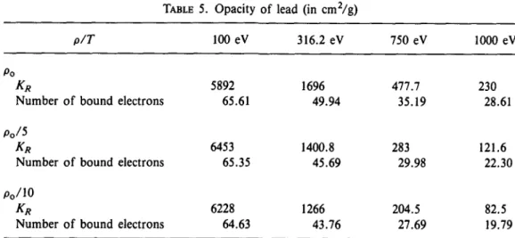
In Table 5 we present total Rosseland opacities and numbers of bound electrons in the case of lead. As regards the opacity, we observe at most the 30% difference between gold and lead. Let us first remark, however, that one should in principle compare opacities for the same pressure and not these at the same density in units of p0. We noticed in

TABLE 5. Opacity of lead (in cm2/g) P/T

Po

KR

Number of bound electrons Po/5

KR

Number of bound electrons Po/10

KR

Number of bound electrons

100 eV 5892 65.61 6453 65.35 6228 64.63 316.2 eV 1696 49.94 1400.8 45.69 1266 43.76 750 eV 477.7 35.19 283 29.98 204.5 27.69 1000 eV 230 28.61 121.6 22.30 82.5 19.79

the case of lead the presence of bound states with large principal quantum number, even up to n = 14. This is connected with the fact that the solid densities of lead and gold are different. For instance in the case of p = po/10 we have for the normalized radius (Appendix A):

while that of gold at p0/10 is:

= 38.56

tfM = 31.55.

This high atomic radius in the case of lead leads to a Coulomb-like behavior of the potential tail and to the existence of high n hydrogenic levels. We repeated the calcula-tions in the two above mentioned cases (T= 1000, p = po/l0, and p = po/5) of lead with

neglected upper bound states of higher n.

We checked that the elimination of high n bound energy levels (n > 10) reduces the Rosseland opacity of about 597o (Blenski & Ligou 1988c). Let us add also that in the case

T = 1000 eV, p = p0/10, the number of (bb) transitions was initially 742 and became

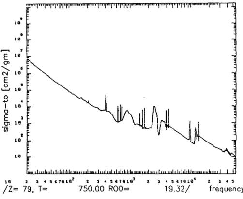
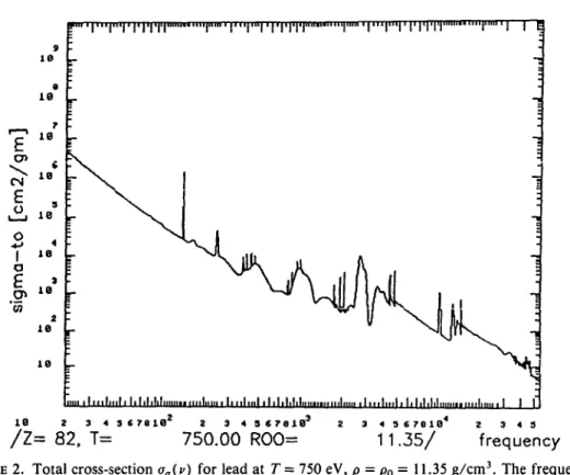
408 when the bound states taken into consideration were limited by the condition n < 10. On figure 1 and figure 2 we present two examples of total cross sections aa{v): the

first (figure 1) for gold at T = 750 eV, p = p0, the second (figure 2) for lead at the same

conditions.

'T""1!' _{MM'l'ir 1 A}

ii.... I,,,I,,.1,1,1,1,1,1,,, ml I,,,I,,,I,I,I, ,,[„,,. .I,,,l,,,l, innnl I I'

10 2 3 4 3 6 7 8 1 0 2 3 4 5 * 7 8 1 0 2 3 4 3 6 7 8 1 0 2 3 4 3

/ Z = 79, T= 750.00 ROO= 19.32/ frequency

FIGURE 1. Total cross-section aa(v) for gold at T = 750 eV, p=po= 19.3 g/cm3. The frequency is ineV.

272 T. Btenski and J. Ligou iiimlniliiililililililiiMiiiiiiiiliiiiiiliiiliiililililililiiiii ilitiii.linliiililililililiiiiiinniiliiiii.l I 10

/ Z = 82, T=

11.35/ frequency

Acknowledgment

Helpful discussions with Dr. B. Cichocki are gratefully acknowledged. We wish to thank Roland Calinon and Marek Swierkosz for their assistance in the initial phase of the nu-merical work for this study.

This paper has been supported by the Swiss Science Fund through subsidy 2.413-0.85.

REFERENCES

ABRAMOVITZ, M. & STEGUN, I. 1965 Handbook of Mathematical Functions (Dover Inc., New York).

ARMSTRONG, B. H. & NICHOLLS, R. W. 1972 Emission, Absorption and Transfer of Radiation in

Heated Atmospheres (Pergamon Press, Oxford).

BETHE, H. A. & SALPETER, E. E. 1957 Quantum Mechanics of One- and Two-Electron Atoms (Springer-Verlag, Berlin).

BtENSKi, T. & CICHOCKI, B. 1988 in preparation.

BLENSKI, T. & LIGOU, J. 1988a Computer Physics Communications 50, 303-311.

BLENSKI, T. & LIGOU, J. 1988b Radiation Opacities for High Z Elements 19th ECLIM, 3rd-7th October 1988 Madrid.

BLENSKI, T. & LIGOU, J. 1988c Average atom calculations of Radiation Opacities for Gold of High Density and Temperature, presented at Fourth International Workshop, Atomic Physics for

Ion Driven Fusion, Orsay, 20-24 June 1988.

CARSON, T. R., MAYERS D. F. & STIBBS, D. W. N. 1968 Mon. Not. R. Astronom Soc. 140, 483.

Cox, A. N. 1965 Stars and Stellar Systems, L. H. Allen and D. B. McLaughlin eds. (University of Chicago, Chicago), Vol. 8, p. 195.

HERMAN, S. & SKILLMAN, S. 1963 Atomic Structure Calculations (Prentice-Hall, Inc., Englewood Cliffs, New Jersey).

LATTER, R. 1955 Phys. Rev. 99, No 6, 1854.

LONG, K. A. & TAHIR, N. A. 1987 Phys. Rev. A 35, No 6, 2631.

MERMIN, D. 1965 Phys. Rev. 127 No 5A, A 1441.

NARDI, E. & ZINAMON, Z. 1979 Phys. Rev. A 20, No 3, 1197.

POMRANING, G. C. 1973 Radiation Hydrodynamics (Pergamon Press, Oxford).

PRITZKER, A., DRESSLER, K. & HAELG, W. 1975a J. Quant. Spectrosc. Radiat. Transfer 15, 1131. PRITZKER, A., HAELG, W. & DRESSLER, K. 1975b / . Quant. Spectrosc. Radiat. Transfer 16, 629. ROZSNYAI, B. F. 1972 Phys. Rev. A 5 No 3, 1137.

SHALITIN, D., STEIN, J. & AKIVA R. 1984 Phys. Rev. A 29, No 5, 2789.

WEBER, S. 1987 Diploma thesis, EPFL, Lausanne.

Appendix A: Thomas-Fermi atom of finite temperature and density (Latter 1955)

The basic assumption is that the phase space distribution of electrons has the form of a local Fermi-Dirac function:

f

.

Ar,p)drdp = -p

where E{f,p) is the classical energy,

E(f,p) = £- - eV(F); (A2) 2m

T is the temperature, a the chemical potential, h the Planck constant, and the factor 2

in equation Al accounts for two spin possibilities. The electron density is found as

• /

p(r) = \d3pfTF.(r,p),

and it is related to the potential by the Poisson equation:

V2KTF.(f) =4irep(r) (A3)

(in equations A2 and A3, the electron charge e is positive). The boundary conditions for equation A3 are:

VT,p.(r) » — for r = \r\ -» 0; (A4) and VFT.F.(r) = 0 for \r\ > r0; (A5) where / 3 V/3 ro= ( - i - ; (A6)

with na being the atomic density.

By the substitution of equation A2 into equation Al, equation A3 is transformed into a nonlinear differential equation:

274 T. Bteriski and J. Ligou

l6ir2e(2mT)3/2 w \eVr_F.(r)

(A7)

n- L 1 j

where

'»<*>=r.--,.

r f j y

",. .• (AS)

Jo^o cxpi^ — x] + 1

We now introduce the dimensionless variables x and x(*):

r = xaobZ-m; (A9)

where

6 = - l — J = 0 . 8 8 5 3 . . . ;

and a0 is the Bohr radius.

The dimensionless form of equation A7 has then the following form:

; (All) with the boundary conditions:

X(O) = 1; (A12) d . . *(*,) (A14)

rfx " xo

The chemical potential is obtained from the condition of electric neutrality of the sphere of radius r0:

2Z4 / 3 Y<xn)

a = —-— EQ . (A16)

b x0

An efficient algorithm of solution to equations A11-A13 consists of transforming them into an integral equation and then using a shooting method. It is described in Latter (1955).

Appendix B: The photon cross-sections

Only final formulas are given in this Appendix. They are obtained from the Fermi Golden Rule (Armstrong & Nicholls 1972) (see also Carson et al. 1968; Blenski & Ligou 1988) and a number of simplifying assumptions:

1) The independent particle model for electronic states 2) Single photon processes

3) Dipole approximation

4) Spherical symmetry and closed shells

5) Fermi-Dirac statistics for occupation of energy levels with the T.F. chemical poten-tial given by equation A16.

aa(v) = abb(v) + abf(v) + aff(v); (Bl) obb(V) = hv £ Labfab{hv -Eb + Ea)\(RnaJa\r\Rnb>lb>\2; (B2) no,loa0 Ea.Eb<0 obf(v) = hv £ Lab6(hv + Ea)\(RnaAa\r\REa+hvAb)\2; (B3) na.laa0 Ea<0 of/(v)=hvZ f dEaLab\{REaAa\r\REa+hvAb)\2; (B4) loa0 Jo where 4ir2

Lab = — a,|8i..i6+i + 8i..i6-i| 2max(la>l6)F(£o)(l - F(Ea + hv));

F(E

)= [

p ( £ y ^ + l ] ; (B5)

ots is the fine structure constant, Ea, Eb are the energies of initial and final states,

re-spectively, la, lb are their corresponding angular quantum numbers; fab(hv - Eb + Ea)

is the line shape function of the transition a -» b (see Appendix C); 6 is the Heaviside function:

fl, x> 0;

6(x) = \

10, x<0.

Rno,\a (r) is the radial part of the electron wave function of the bound state

character-ized by the quantum numbers na and lo.

where YXatma {6,<p) is the spherical harmonic, /?£0,i0 is the radial part of a free state

elec-tron wave function of energy Ea,

. . . * . .( I l M B( 0 , * ) . (B7)

The bound electron wave functions are normalized in the usual way:

276 T. Bteriski and J. Ligou

(Rna,\a\r\Rnb,\b) denotes the radial matrix elements of r:

<Rna,O\r\Rnb,lb> = jdrr2RnaAa(r)rRnbAb(r); (BIO)

The radial wave functions are calculated from the following dimensionless Schrodinger equation:

D(x) - ^ ] J A , , W = 0 (Bll)

where the sign ± corresponds to a free (bound) state;

v(

) = 2 Z - J*M _ *!*>> \

\ X Xo )

and xix) is defined by equation A10.

The functions A , I ( * ) a fe related to the radial wave functions as follows:

where

f -\2Z2/3/b2E0, for bound state;

Ex =\ (B14)

\\2Z2n/b2E0, for free state.

The equations B9-B10 and the above definition lead to:

5nh', Ea,Eh < 0

The numerical solutions of equation Bll are needed for xe [0,x0]. Beyond x0, both bound

and free wave functions may be found analytically in terms of Bessel functions (Abramovitz & Stegun 1965). The formula and numerical schemes for the bound states may be found in BJeriski and Ligou (1988a).

In the case of a positive energy wave functions we have

y(x) = xlAJ^Xx) + BiyiCKx)]; x > x0; (B16)

where j\(z) and.)>i(£) are Bessel functions and A1; B, unknown coefficients. The

inte-gration of equation Bll, for x < x0, only yields the phase shift modulo ir:

The second equation for A] and Bi follows (Carson et al. 1968) from the asymptotic be-haviour of the Bessel functions (Abramovitz & Stegun 1965). One obtains finally:

Jo (B18)

Bi = l +XQ 2 ; (B19)

Ai = D\BU

The matrix elements may be calculated from the dipole form, equation BIO, or from an equivalent expression:

4 72 / 3/ >

' ' • " ' ( B 2 0 )

(±Xft ± X2,) Jo dx I x

where x{x) is defined by equation AlO and the upper (lower) sign corresponds to a free (bound) state.

Appendix C: Thomas-Fermi theory of band formations

Our approach to the absorption band formation is of fully statistical nature. We use the fact that the temperature dependent version of the T.F. theory may be found by minimi-zation of a grand thermodynamical potential fi (Mermin 1965):

8il[p] = 0 (Cl)

As in Shalitin et al. (1984) we consider now small fluctuation of electron phase space density as perturbation to the T.F. phase density/T.F.(r,/?) (equation Al):

f(r,P) =fr.?.(r,p) + 8f(r,p). (C2)

The total electrostatic potential is now:

V{r) = y + Vr.F.(r) + 8V(r); (C3)

with

where

5p(r) = jd

p$f(F,p). (C5)

The first order perturbation to the energy level E, is:

fe, = E, - E7

- = -J\iF{r')\

e8V(F)d

r';

= e J Vi(r)8p(r)dr; (C6)

M ;

(C7

,

278 T. Bteriski and J. Ligou

where ypJF(r) and E, are the wave function and energy of the /'-th bound state of the

T.F. potential. Retaining only the first term in the multipole expansion:

1 _{= - + . . . ; (C8)} \r-r'

one gets:

Vi(F)

= _

UrW-inr.

where

The probability distribution of the density fluctuation bp(r) can be expressed, in the frame of a density functional approach, as being proportional to exp where b2Q is a

bilinear functional of 5p(r). The formalism finally leads to the following probability dis-tribution for the energy fluctuations (Bteriski & Cichocki 1988):

P[{bek}] =Cexp\-^AijbeibeJ] (CIO)

where the matrix Ay depends only on nT F (r).

In this paper, we neglect the off-diagonal elements of Ay and do not take into account nonlocal terms in 52Q. Finally, we average aa(v) with P [{beK}] given by equation CIO

and neglect all the energy dependence except the energy arguments in the Dirac delta ap-pearing in equation B2.

We get for the averaged dbb(v~):

[«(e,)(l - n^jM^hu) (Cll) where

Mhv) = (2ir(bEfj))-1/2exp\ — (hv - A0)2/(bEfj) (C12)

with

A,7 = Ej-r- - Ej*- (C13a)

(bEfj) = (bEf) + (bEf) (C13b) (bEf) = - , , e2 I c

The same formula for <5£",2> (equation C13c) (larger by the numerical factor of 2) has been obtained by Shalitin et al. (1984) by a different way. The present derivation gives, however, in addition to equation C13c, the Gaussian function equation C12 and leaves therefore no ambiguity in the interpretation of (bEfj) (the interpretation of (bEfj) as the halfwidth would lead, for example, to a different numerical factor in equation C12).

Appendix D: Oscillator strength sum rules

The derivation may be found in Bethe and Salpeter (1957):

3 2 / + 1 '

3)

2 / + 1

(Dl)

(D2) The upper indices are related to final states, the lower to the initial ones. The summation is upon all final states.

With our normalization the LHS of equations Dl and D2 have the following explicit forms: dKj Jo Jo (D3) fn',l-\ _ 1 / 3 2 / + 1 / • Jo L £„-,/_ i<0 • (D4)