Computational and visualization techniques for Monte Carlo based SPECT

Computational and Visualization Techniques

for Monte Carlo Based SPECT

A.B. Dobrzeniecki and J.C. Yanch

Whitaker College of Health Sciences and Technology

and Department of Nuclear Engineering, Massachusetts Institute of Technology,

Cambridge, MA, USA

e-mail: andy@rad.mit.edu, jcy@imager.mit.edu

25 January 1993

I

Abstract

Nuclear medicine imaging systems produce clinical images that are inherently noisier and of lower resolution than images from such modalities as MRI or CT. One method for improving our understanding of the factors that contribute to SPECT image degradation is to perform complete photon-level simulations of the entire imaging environment. We have designed such a system for SPECT simulation and modelling

(SimSPECT),

and have been using the system in a number of experiments aimed at improving the collection and analysis of SPECT images in the clinical setting. Based on Monte Carlo techniques,

Sim-SPECT realistically simulates the transport of photons through asymmetric,

3-D patient or phantom models, and allows photons to interact with a number of different types of collimators before being collected into synthetic SPECT images. We describe the design and use of SimSPECT, including the compu-tational algorithms involved, and the data visualization and analysis methods employed.

Keywords: Medical Imaging, SPECT Modelling, Scientific Visualization, Medical Physics.

Contents

1 Introduction 4

2 Background

4

3 SPECT Simulations with SimSPECT

6

3.1

SimSPECT Applications ...

9

3.1.1

Correction for Scatter and Attenuation ...

9

3.1.2

Noise Analysis . .. ...

...

.. .. .. . 10

3.1.3

Collimator Design and Evaluation . . . 10

3.1.4

Radiopharmaceutical Design and Analysis . . . 12

3.2

SimSPECT Algorithms . . . 12

3.2.1

Sim SPECT . . . 13

3.2.2

Sim SPECT(n) . . . 19

3.2.3

SuperSimSPECT . . . 23

3.3

SimSPECT Implementation . . . .. . . 27

4 SimSPECT Performance

28

4.1

Data Requirements . . . 30

4.2 Time Requirements . . . 30

4.3

Comparison with Related Systems . . . 32

5.1

SimVIEW Image Processing . . . 33

5.2

Visualization of SimSPECT Data with SimVIEW . . . 36

6 Summary and Conclusions 39 7 Future Work 39 8 Acknowledgements 40 References 40

List of Figures

1

Capabilities of the SimSPECT system. . . . .

7

2 Comparison of clinical and synthetic SPECT data . . . . 8

3 Simulated hollow spheres phantom data . . . . 9

4 Noise Power Spectrum and RMS noise for a flood phantom . . . 11

5

SimSPECT design . . . 14

6

SuperSimSPECT architecture . . . ... . . . 25

7

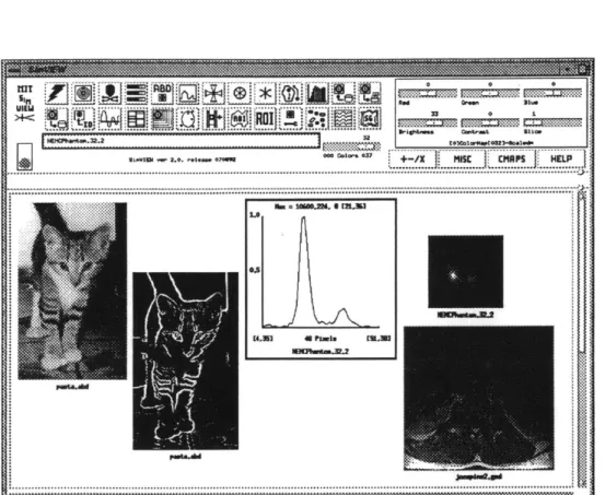
Sim VIEW system screen . . . 34

8

Sim VIEW selection box for SimSPECT data . . . 37

List of Tables

1 Functions performed by SimSPECT modules . . . 29 2 SPECT data storage requirements . . . 30 3 SimSPECT run-times . . . 31

I

1

Introduction

Simulation of the complete nuclear medicine imaging situation for SPECT (Single Photon Emission Computed Tomography) produces synthetic images that are useful in the analysis and improvement of existing imaging systems and in the design of new and improved systems. The simulation methods that we employ are based on probabilistic numerical calculations; they require enormous amounts of computer time and employ highly complex models (the tomographic acquisition of images through intricate collimators). Described here are the techniques we have developed to achieve reasonable simulation times, and the tools we have built to allow interactive and effective analysis and processing of the resultant synthetic images. The computational algorithms involve innovative methods of subdividing the particle transport problem and solving it in parallel on heterogenous computer platforms. The visualization tools for manipulating synthetic images permit interactive exploration of the underlying physical factors affecting image acquisition and quality.

2

Background

Numerous factors affect the ultimate qualitative and quantitative attributes of images acquired from nuclear medicine studies. These factors include the composition of the collimator, the varying scatter and attenuation rates in the source objects, and the controllable imaging parameters, such as source-to-detector distance, energy windows, and energy resolution in the gamma camera. Because the effects of these phenomena cannot be easily studied in an experimental setting (either due to cost or physical impossibility), one way to study such effects is to perform simulations of the entire imaging situation. Such simulations can provide data (via synthetic images) that can be used to individually examine the origins of degradation in nuclear medicine images, to design methods to mitigate such effects (scatter correction and attenuation correction algorithms, etc), and to analyze new imaging systems regarding feasibility and performance characteristics.

Simulations of medical imaging systems can proceed along two paths, using either analytical or statistical models. Analytical solutions are generally avail-able only for highly constrained models, such as spherically symmetric source

objects; such solutions, although exact, are unable handle the many complex interactions that occur between particles and matter during the generation of images [11]. Statistical methods, however, allow a complete and realistic treat-ment of all interactions of radiation with matter, but at the cost of increased computation time. Most statistical simulations employ numerical techniques based on the Monte Carlo formalism to model the transport and interaction of particles within a medium. Monte Carlo techniques, as applied to nuclear medicine [1], produce estimates of the average behavior of particles by tracking a representative number of particles from their birth to their eventual capture, with scatter and other types of interactions modelled along the way. Monte Carlo calculations are so named because of their random nature; that is, the probability of some interaction between a particle and some medium (a scat-tering collision, for example) is dependent on a throw of the dice to determine into what angle the particle is scattered, for example. Monte Carlo trans-port methods also require vast amounts of physical data, such as scattering probabilities as a function of material density and photon energy.

Monte Carlo techniques fall under the general heading of transport theory methods; transport theory attempts to solve problems dealing with the move-ment of particles in space and time, and solves the Boltzmann transport equa-tion. By producing an estimate of the average behavior of all photons by sam-pling the behavior of a representative fraction, Monte Carlo methods provide solutions to transport problems without actually referring to the Boltzmann equation. As larger and larger numbers of photon histories are tracked, the accuracy of the solution to the transport equation becomes more and more ac-curate. Thus, Monte Carlo methods present an inherent tradeoff between the large commitment in computer time and the degree of agreement possible with physical reality. In the work described here, we have focused on reducing the computational costs of Monte Carlo methods, without sacrificing the realism of generated images.

In SPECT modelling, once a statistical simulation of transport processes has been performed, the synthetic images obtained can be analyzed to determine the sources of image degradation due to collimator geometry, photon scatter effects, and other factors. Ideally, the simulation techniques must yield syn-thetic data that are flexible enough to permit many experiments to be carried out with a single set of data; this requirement stems from the large computa-tional times needed to perform any one realistic simulation. That is, if every change in the collection energy window, for example, necessitates a new

sim-I

ulation run, the total time will be prohibitive for investigating energy window effects on resultant images. Thus, we would like the synthetic data from sim-ulations to be useful for a variety of experiments and analyses; the methods for visualizing and manipulating such data should therefore be effective and flexible.

In the following sections, two applications are discussed in detail that address the two research areas mentioned above, specifically the generation of synthetic medical data and their visualization. The first application, named SimSPECT,

allows the generation of physically realistic synthetic Nuclear Medicine images; the methods that are used in SimSPECT to achieve reasonable computational speeds for very large simulations will be presented. The second application,

Sim VIEW, is an image processing and visualization tool that permits the rapid

and effective exploration of the large data sets generated by SimSPECT. Al-though both SimSPECT and SimVIEW are currently being used in a variety of research and development projects, the focus here will not be on applica-tions of the systems, but rather on the algorithms and designs used in building and running the systems (several applications will be presented only to give a general overview of how these systems are used in research and development endeavors). Furthermore, the SimSPECT system is not a single application, but consists of a number of related systems that have been evolving over time; this chronology of changes and algorithmic improvements to SimSPECT will also be presented.

3

SPECT Simulations with SimSPECT

SimSPECT is a simulation package for SPECT imaging systems that achieves the following goals:

e Completely and realistically models interactions between emitted

pho-tons and transport media.

e Allows use of source material and scatter objects of arbitrary composition

and arbitrary 3-D geometrical shape.

e Employs models of collimators that correspond exactly to clinical or

Planar Image

HighRas Collimator: 85,006

hex-packed holes (1.1 ma dia) in a slab of lead 39 cn by 39 cm by 2.3 am thick Compton Scatter Followed by Photon Capture Collimator Source

Objects _{Compton Scatter in Air}

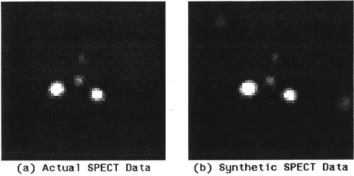
(a) Actual SPECT Data (b) Synthetic SPECT Data

Figure 2: Comparison of clinically obtained phantom data (a) and synthetic

SPECT data (b).

Figure 1 illustrates the capabilities of the SimSPECT system: differing types

of interactions are modelled, complex collimators are employed, asymmetric

source and scattering objects are present, and data acquisition is in three

dimensions. Figure 2a shows a simulated SPECT image of several solid spheres,

filled with a Tc

9 9_M

_{solution, in a cylindrical water phantom. Figure 2b is}

an actual image obtained using a clinical SPECT system. The agreement

between synthetic and actual data is excellent, and verifies the accuracy of the

SimSPECT simulation. Further descriptions and validations of SimSPECT

can be found in [12] and [13].

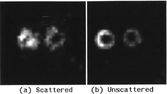
Figure 3 shows the reconstruction of two small hollow spheres containing T

201

in a bath of water, using only those photons that did not scatter in the

phan-tom (Figure3b) and those photons that did undergo at least one interaction

(Figure3a). Such images are not available experimentally, and only through

simulation is it possible to begin to quantitatively assess the degradation and

noise of a final image due to photon scatter (both in the collimator and in the

source/transport media). We are currently using SimSPECT to assemble sets

of gold standard image data for various types of phantoms, radioisotopes and

collimators; using such data sets, concepts and techniques can be tested in a

manner that is not possible with experimenatlly acquired data.

I

(a) Scattered

(b) Unscattered

Figure 3: Hollow spheres phantom. (a) Simulated image using only photons

that have undergone scattering; (b) only photons that have not scattered.

3.1

SimSPECT Applications

Given the capability to completely and realistically model the SPECT imaging

process, certain design and analysis tasks become possible; in this section,

sev-eral research efforts are described that rely on SimSPECT for data generation

and concept validation.

3.1.1

Correction for Scatter and Attenuation

Photon attenuation and scatter are important sources of image degradation

in SPECT, with many methods having been proposed as corrections for such

effects [3, 7]. For example, manipulations of photopeak data often focus on

estimating scatter fractions at various energies, and then either reject photons

with high probabilities of having scattered or reduce their importance [4, 9]

We are currently using SimSPECT to assess the accuracy and performance of

a novel Bayesian estimation method for scatter correction; by knowing precise

scatter fractions and the locations of scattering events for individual photons

(such as in the collimator, in the source object, or in the transport medium),

such a scatter compensation algorithm can be evaluated absolutely without relying on qualitative image characteristics; this work is in progress.

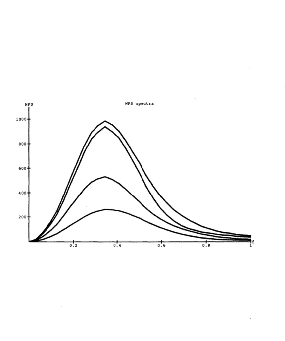
3.1.2 Noise Analysis

A related application of SimSPECT data is the characterization of the noise inherent in SPECT images. Figure 4 shows the noise power spectrum for a flood phantom at differing count levels for synthetic data. Although the noise parameters shown are for images containing scattered and unscattered photons, similar analyses can be readily performed using data containing only scattered photons. Separating scattered photons from unscattered photons is feasible when using SimSPECT synthetic images. Such studies, which are in progress, are expected to yield details on the nature and correlation of noise in SPECT images, and to further validate the accuracy of SimSPECT simulations. In addition, we plan to evaluate the effects on SPECT noise of various computational improvements to the Monte Carlo process (such as importance sampling, which is a variance reduction technique that increases computational efficiency in Monte Carlo transport methods [5]).

3.1.3

Collimator Design and Evaluation

Collimator designs are often difficult and expensive to test experimentally. For example, by making the septal thickness smaller for a given collimator, the ef-ficiency of photon collimation can be increased. However, as septal distances shrink, the number of photons that scatter through the collimator and reach the scintillation crystal increases. Such scattered and detected particles de-crease the quality of resulting images, and an accurate measure of this effect can aid in assessing the effectiveness of a particular collimator design. The following are areas in which such simulations of collimators are important and are being done (or planned) using SimSPECT:

* In many studies involving small animals, higher dosages of radiophar-maceuticals are allowed than for human patients; such higher fluxes of particles mean that less efficient collimators can be used, but also that septal distances can be increased to limit image degradation due to scat-ter. The optimal tradeoff between collimator efficiency and image quality

NPS NPS spectra 1000 800 600 400 200-0.2 0.4 0.6 0.8

Figure 4: Noise Power Spectrum for a flood phantom for scattered and

un-scattered photons at differing count levels.

can be determined via simulation prior to constructing a small-animal camera.

* Radioisotopes that emit low energy gammas (such as

P25)

often have desirable properties for use in small-animal imaging. However, these low energy photons are heavily absorbed in lead collimators, and result in excessively noisy images of poor quality. Thus, materials other than lead may be appropriate for collimators for I.2s imaging, and the properties of such collimators (and their design) can be assessed by simulation trials. " Focusing (cone beam) collimators can improve the collection efficiency of a given imaging agent; however, many aspects of focusing collimators have not been studied in detail. For example, depth-of-field effects that result from focusing the emitted photons can cause severe image blurring, and through simulations these effects can be estimated or compensated for.

3.1.4

Radiopharmaceutical Design and Analysis

A final application of SimSPECT involves the analysis of novel radiopharma-ceuticals designed for the detection of coronary artery disease (atherosclerosis); such lipid-based agents are still under development [8], and will probably pro-duce images of extremely low contrast and high noise. Using simulations of the entire imaging system, the limiting target-to-background ratios can be spec-ified for a given radiopharmaceutical such that the resultant SPECT images are clinically productive. The determination of these minimal performance requirements is currently being carried out using SimSPECT.

3.2

SimSPECT Algorithms

The essential photon tracking and interaction algorithms contained in

Sim-SPECT are from an embedded Monte Carlo transport code, MCNP.

Devel-oped at Los Alamos Scientific Laboratory, MCNP represents the state-of-the-art in terms of the physics, cross-section data, and models necessary for photon Monte Carlo simulations [2]. MCNP contains photon cross-section tables for materials with Z = 1 to Z = 94, and these data allow MCNP to simulate inter-actions involving coherent and incoherent scattering, photoelectric absorption

with emission of characteristic xrays, and pair production with emission of annihilation quanta. Thousands of hours of development and use have ren-dered MCNP a transport code which is thoroughly debugged and validated [10]. MCNP also has a generalized input file facility which allows specification of an infinite variety of source and detector conditions, without having to make modifications to the transport code itself. This user-defined input file defines the size, shape and spectrum of the radiation source, the composition and configuration of the medium through which photons are transported, and the detector geometry and type. Using the MCNP geometrical primitives, a user can construct three dimensional source and transport media whose complexity and realism approach the physical objects being modelled (a human brain, for example, including gray/white matter, blood vessels, ventricles, skull, etc). All aspects of photon transport in the source objects and the collimator are modelled in SimSPECT. The detection crystal is not modelled, but once a pho-ton reaches the face of the crystal, after having passed through the collimator, the photon's energy and spatial position are modified to simulate the effects of a given scintillation detector. That is, the photon's energy is sampled against an inverse probability density function (PDF) with a variance derived from the FWHM for that type of detector. For example, given a photon impinging on a scintillation crystal with energy E, the energy after sampling against the inverse PDF is E'; performing the sampling many times for the same value of E, and plotting the E' values, gives a gaussian curve centered on E with a FWHM equal to K kev. This curve represents the energy spreading that is encountered when detecting monoenergetic particles by an actual scintilla-tion detector; for GaAs detectors K is on the order of several key, whereas for the common NaI detectors K ranges from 10 to 20 key. Likewise, spatial spreading is performed on the photon's position when it reaches the face of the scintillation crystal; this convolution step simulates the blurring that is apparent in actual detectors'. The energy spreading and spatial blurring steps are performed differently in each of the SimSPECT systems; these differences are discussed in Section 3.

iThe spatial blurring phenomenon is an extremely small effect; it is not the point spread phenomenon due to detector geometry.

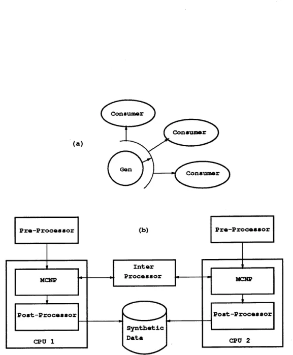
(a)

Figure 5:

(a)

SimSPECT concept of photon Generators and Consumers. Photons emerging from the source/transport media in the photon Generator are cloned and redirected to photon Consumers for interaction with a colli-mator and contribution to a tomographic image. (b) General schematic of the

3.2.1

SimSPECT

Development of the SimSPECT system began with the creation and addition to the core MCNP code of a pre-processor, inter-processor, and post-processor. The pre-processor permits user-friendly generation of source and transport ob-jects, and eliminates the need to directly specify complex geometrical forms such as collimators2_{. The inter-processor modifies the internal tracking and}

manipulation of photons such that synthetic images can be created, and con-trols this task so that it can be accomplished using multiple CPUs. The post-processor assembles the final synthetic SPECT data, and manages ad-ministrative information regarding the simulation. The general architecture of the SimSPECT system is shown in Figure 5b (for a run utilizing two CPUs). The need for a SimSPECT pre-processor was, simply, to create a less cum-bersome mechanism for specifying the relevant parameters for SPECT sim-ulations. These parameters are placed in a special input file which the pre-processor converts into an expanded data file that is then read by the

Sim-SPECT system to determine configuration and simulation details. Collimators

can be described to the pre-processor by indicating the type of collimator (par-allel hole, cone-beam, etc), the number of holes in the collimator, the shape of the holes (round, hexagonal, square, etc), the packing of the holes (rectangu-lar or hexagonal packing), the septal distance between holes, and the overall size of the collimator (FOV and depth). Patient/phantom models and source distributions are also defined in the input file, as are other parameters such as the number of tomographic views to collect, the number of CPUs to use, and the number of photons to track.

The post-processor likewise satisfies the rudimentary need of managing large amounts of simulation data. The post-processor assembles simulation data into relevant image files, and handles the restarting of long simulation runs that have been terminated due to power failures, network errors and other occurrences. During a simulation run, when a photon reaches the detection crystal, the post-processor increments the corresponding pixel value in the relevant synthetic image; a different image is created for photons that have scattered versus those that have not scattered, and for photons that are within

Designing a cone beam (focusing) collimator with hexagonal holes packed in an hexago-nal requires over 10,000 lines in the MCNP input file, whereas using the pre-processor such a collimator can be specified with only a few directives.

a user-defined energy window versus those outside the window3_{. Determining}

whether a photon is within an energy window is carried out after the photon's energy is sampled against an inverse PDF that models the crystal's energy resolution properties.

The inter-processor is a key component of the SimSPECT system, and has been evolving over time to allow simulation runs to proceed with the greatest speed, efficiency and effectiveness. The design of the inter-processor was predicated on the observation that in order to simulate tomography for asymmetric source and problem geometries, it is necessary to run the simulation n times to collect n tomographic images. Thus, in order to simulate p disintegrations in a source object per tomographic view, it is necessary to generate and track a total of np photons. If the average time to follow a single particle from birth to eventual capture or escape is t, then the total time for a simulation requiring p disintegrations per tomographic view is T = npt. For a typical number of disintegrations (p = 100 x 106), a standard number of planar tomograms (n =

60), and an average photon tracking time (using SimSPECT and MCNP) on a fast, single-CPU workstation (t = 2 msec), the total time required to perform such a baseline SPECT simulation is approximately T = 139 CPU days.

These long run-times are clearly prohibitive for exploring SPECT imaging systems. Typically, with 100 x 106 disintegrations per tomographic view, the resultant images contain approximately 10, 000 counts per view.

There are several obvious ways to reduce the time required to collect n tomo-graphic views, but none is completely satisfactory or applicable. For example, one method is simply to put an array of n collimators/detectors around the source geometry and thus reduce the total number of photons to be tracked to just p. However, this method is not viable because collimators are geometri-cally complex and require significant amounts of computer memory to model; also, if n is close to the value used in clinical SPECT (n = 30 to 60), there is significant collimator overlap in space which makes it difficult to correctly track photons4. The initial method we have chosen for simulating tomography in

3_{Specifically, five image files are created per tomographic view for photons that have}

reached the detector: 1) all photons, 2) photons that have not scattered and are inside the energy window, 3) photons that have have scattered and are within the energy selection window, 4) photons that have not scattered and are outside the energy window, and 5) photons that have scattered and are outside the energy selection window.

4

Because SimSPECT uses MCNP's internal geometry modelling facilities, which do not allow structures to overlap in space, it is impossible with the current system to represent all collimator positions simultaneously during a single simulation run.

an efficient and rapid manner (in SimSPECT) makes use of multiple processes running on separate CPUs and is schematically illustrated in Figure 5a. One process is designated the photon Generator, which tracks photon interactions within the source and transport media (patient or phantom). When a particle leaves this space and passes through a virtual sphere surrounding the space, its position, direction, energy, and scatter order are saved. The photon is then cloned and allowed to interact with the collimator for all views with which it would interact. This step is carried out by one or more photon Consumers using separate CPUs, as shown in Figure 5b. Thus, only a single model of the collimator is required per Consumer; during the photon cloning process, particles are redirected to this single model of the collimator, but counted for the actual tomographic view corresponding to the original photon direction. This method achieves a degree of coarse-grained parallelism, and can produce tomographic simulations in a time less than for the baseline case, i.e, T,

<

npt. Specifically, the total time required to track p photons per tomographic views through their entire lifetime in SimSPECT is

T,

=

p(tg

+

qth + ),

(

q

with q being the number CPUs available, p the number of photons to be tracked (the average number of disintegrations to be simulated for a given tomographic view), n the number of tomographic views to be acquired, tg the

average time required to process a single photon through a Generator, te the average time required to process a single photon through a Consumer, and th

the average overhead (time) per photon due to the use of multiple CPUs. Note that the total time, T, for a simulation run does not represent the sum of all processing time on all CPUs, but rather is the largest linear block of time for the simulation. Thus, given q CPUs, T, is time we would measure on a clock as being required to complete a simulation task, although the total amount of time used by all the CPUs would be somewhere between T, and qT,. T, is

therefore referred to as the total linear time.

As the number of processors used goes up, processing time per photon decreases because more cloned photons are tracked in parallel. However, each additional processor increases the amount of time that is spent managing the multiple processors and communicating among them (the total overhead time). That is, as the number of processors goes up, the processing time per photon decreases

and the overhead time increases per photon, until the increased overhead is not offset by the decreased processing time. This balance point is found by setting

BT,

a

0. (2)

Combining (1) and (2) yields

qopt = C

(3)

where q,,t is the optimal number of Consumer processes that results in the shortest linear time for execution of a simulation run5.

Based on observations of the performance of the SimSPECT system for a number of different problems and running on a variety of hardware platforms, we estimate the following values for the parameters necessary to calculate qt and T,; these values are normalized for a machine with a MIPS CPU with a

rating of 3.0 MFLOPS

p

= 100 x 106

photons,

q = _{2, 4, 6, or 8 CPUs,} n = 60 tomographic views, (4) t= 1.0 msec, te= 0.7 msec, th = 0.3 msec.

Thus, a typical SimSPECT simulation run with two processors (one photon Generator, one photon Consumer), requires 26 days of linear CPU time.

The optimal number of processors, qopt, is approximately 12 (one Generator,

11 Consumers), for which T, would be 9.4 CPU days.

sSeveral simplifying assumptions have been made for this analysis, for example, that the speed of each CPU is identical, and that the overhead time per photon is a constant.

For comparison, the baseline method of performing a similar simulation (ac-quiring one projection image at a time) requires

T,

= pn(tg

+

tc),

(5)

and for parameters given in (4) above, this yields a T, of over 118 CPU days! Clearly, both the baseline approach and SimSPECT require enormous amounts of computational time to complete a simulation run.

3.2.2

SimSPECT(n)

In a version of SimSPECT named SimSPECT(n), we have reduced the required number of tomographic views that must be simulated by an order of magnitude. This is done by cloning a given photon and sending it to a Consumer process for those photon directions that are nearly perpendicular to the surface of the collimator'. For a typical clinical SPECT acquisition, the distance from the center of the object being scanned (the patient), to the face of the collimator is from 20 cm to 50 cm. Given a collimator with a planar size of 40 cm by 40 cm, it can be shown that any photon impinging on a collimator/detector could have interacted with about half of all other possible collimator positions. That is, in cloning the photons from the photon Generator for the Consumer processes, about half the total number of tomographic views

(n)

must actually be tracked through a collimator; the other half of the photons miss completely the virtual collimator's position. However, if the photon's direction is not within a few degrees of perpendicularity of the collimator, the photon is nearly always absorbed in the collimator; a characteristic xray may result instead of an absorption event, but as these xrays have energies of approximately 80 keo, they will typically not be included in the energy window. Thus, many cloned photons are processed that never contribute meaningfully to the final synthetic image.

Based on SimSPECT runs, we observed that by not tracking photons that were outside a cosine angle of 0.99 of the collimator's face, the resulting images were indistinguishable from those where photons for all directions were cloned and tracked. This is possible because after selection of particles within even a large energy window (30%), the photons that impinged on a collimator with a cosine

angle less than 0.99, and passed through to the detector, had a final energy so low that the particle was always excluded from the energy window. Thus, in SimSPECT(n) there is the capability to set a cosine angle for photon cloning, and this greatly reduces the simulation times with no loss of data fidelity7. For example, a typical simulation with a cosine angle of 0.99 will result in an effective value for n (nff) of 2. Thus, for a SimSPECT(n) run utilizing two processors (one Generator and one Consumer), and with the parameters given in (4), the total linear time for simulation is Tm, = 2.6 CPU days (as compared to a time of 26 CPU days with basic SimSPECT). The optimal number of processors in this case, as given by

(3)

with n ff = 2, is

approxi-mately 3; using more processors than this increases the linear time to complete a simulation task.

The following is another way to understand how SimSPECT(n) reduces the number of photons that must be tracked. Because only a single model of the collimator exists in each Consumer process (due to complexity and size con-straints), every photon that emerges from a source object and passes through the transport media must be redirected to this single collimator; the redirec-tion step preserves the incidence angle of the photon with a collimator located at the original tomographic view. After being redirected, if the photon passes through the single collimator model, it contributes to the image that corre-sponds to the tomographic view to which the photon was originally headed (before redirection). But, given many tomographic views, a randomly ori-ented photon emerging from the source and transport objects can potentially interact with more than one collimator; for 60 tomographic views, a 40 cm by 40 cm field-of-view collimator, and a source-to-detector distance of 20 cm,

collimators at up to 25 different tomographic positions can interact with a given photon. In the original SimSPECT system, each photon emerging from a Generator process was cloned in a Consumer process and allowed to inter-act with all 25 collimator positions. However, in SimSPECT(n), the number of cloned photons is reduced to include only those that would have interacted with a given collimator position by impinging on that collimator within some angle. As this angle (or deviation from a perpendicular path) is reduced, the number of photons that must be cloned drops dramatically. The use of such a technique is valid because, as described above, particles that are not im-pinging on a collimator in a nearly perpendicular direction rarely get to the

7_{0f course, when performing simulations where photon scatter and passage through the}

collimator is important, the cosine angle can still be reduced, perhaps even to 0.0 (all photon directions are cloned and tracked).

8I

scintillation crystal with an energy above the cutoff value8.

SimSPECT and SimSPECT(n) use UNIX interprocess communication (IPC) protocols for managing the distributed computation of photon interactions. As shown in Figure 5a, the single Generator is located on one CPU, and as photons emerge from the phantom/source objects, the photons are cloned and redirected to Consumer processes running on other (or the same) CPUs; each Consumer is responsible for accepting photons redirected to some range of contiguous tomographic views. For example, if 60 views are being acquired, and 4 Consumers are running, each Consumer accepts, on average, photons headed for approximately 15 tomographic views. The inter-processor controls the dispatching of cloned photons (refer to Figure 5b).

The IPC communication functions contained in the inter-processor are used predominantly to transmit photon data (position, direction, energy and scatter order). The communications between Consumers and the Generator are via non-blocking sockets; that is, socket connections are polled to determine their ability to accept a read or write request, rather than waiting for such an acceptance on a given socket. Also, each socket connection serves as both a send and a receive channel, and when any SimSPECT process sends a packet across a socket connection, an acknowledgement is returned by the receiving process; this form of handshaking ensures the integrity of transmitted data, as well as providing a method for determining if a receiving process is functioning properly.

In the Generator, after a photon is born and tracked through the source and transport objects, the photon is ready to be sent to a particular Consumer; if the next Consumer in the queue is still occupied tracking a previous photon,

the Generator tries other Consumers in turn until a successful transfer of the

photon is made. This scheme has two advantages; the first is that it levelizes

the load among Consumer processes, and the second is that it is resistant to

the failure or degradation of any single Consumer process. After a photon

reaches the scintillation crystal in a Consumer process, the post-processor

records the photon's final energy, direction, tomographic view, object scatter

order, and collimator scatter order in a data file which is assembled into a final

set of synthetic images.

8

This acceptance angle is a user-defined parameter, and the SimSPECT system described in [13] is the SimSPECT(n) system referred to here. However, the SimSPECT system in [13] did not implement the ListMode data features described in this section for SimSPECT(n).

The Generator process, and each Consumer process, can be run on separate machines, as long as IPC protocols are available on those machines. Thus, after the SimSPECT system is recompiled on two differing hardware platforms, for example, each machine is available to run either a Generator process or Consumer processes for a single simulation task. Configuring the layout of the SimSPECT system is currently done manually, and requires the user to explicitly indicate how many Consumer processes are required and on what machines the Consumers are to be located. Likewise, should the system need to be restarted in whole or in part (due to a network failure, for example), the restart procedure must be initiated manually by the user.

Unlike SimSPECT, the SimSPECT(n) systems employs a novel method for storing generated SPECT data. In SimSPECT, when a photon reaches the detection crystal, it is counted to a single pixel in the relevant synthetic im-age. Pixel areas are square and non-overlapping, and once a resolution and energy window are chosen, the SimSPECT simulation proceeds with all pho-tons being coverted into counts in respective pixels; this method does not preserve detailed information regarding the photon's scatter order, its energy, or its position. Once simulated SPECT images are acquired, its is only known whether an individual photon underwent any scattering interactions, whether the photon's final energy was within a fixed energy window, and whether the photon's final position fell within the boundaries of some fixed-size pixel. Such pixel-based simulation data is stored in so-called ImageMode files. Thus, be-cause SimSPECT generates ImageMode data, a new simulation run must be be performed each time a new image resolution is desired, or a new energy selection window is needed. In SimSPECT(n), we have replaced ImageMode data collection with ListMode data collection.

In generating ListMode files, the post-processor stores detailed photon infor-mation into sequential list files for all photons that have reached the detection crystal. That is, into a binary file are placed a given photon's position (x and y coordinates are normalized to the range 0.0 to 1.0 -the z dimension is always in the plane of the detector), the photon's absolute energy (no energy sampling against an inverse PDF is performed), the number of scattering interactions in the source objects and transport media, and the number of scattering interac-tions in the collimator. These five values are stored as binary float numbers, and a single ListMode file is created for each tomographic view.

ListMode files are not SPECT images, as is apparent; a way is needed to transform such lists of photons into meaningful images. The Sim VIEW

sys-I

tem, described in detail in Section 5, includes powerful and flexible functions for processing ListMode data. Basically, SimVIEWallows a set of ListMode to-mographic data files to be transformed into pixel-based images (ImageMode data) through user-specified directives regarding final image resolution, en-ergy resolution, scatter orders, and final count levels; the transformation from ListMode data to actual images is instantaneous, versus days of run-time to generate the ListMode data in the first place.

The advantages of simulated SPECT data in ListMode files are obvious; final image resolution can be chosen after a long simulation run has been completed; the energy window (or windows) can be changed and the effects on resultant images can be seen immediately; the energy resolution can be modified to sim-ulate scintillation crystals with differing properties; and finally, the percentage can be set of the photons contained in a ListMode file that are accessed, thus creating images with specified final count levels. In summary, synthetic data in ListMode format allows many more experiments to be carried out after a simulation has been completed than for ImageMode data. The main disadvantage with ListMode data collection is that the data files are greater in size than for ImageMode data. In Section 4, a comparison is made of the

differing storage requirements for ListMode and ImageMode data.

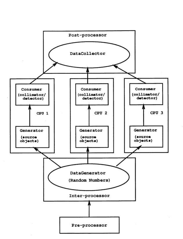
3.2.3 SuperSimSPECT

Although the improvement in processing time is significant from SimSPECT to SimSPECT(n) we are currently working on a version, named

SuperSim-SPECT, that achieves an even greater degree of parallelism and speed. This

version is based on the observation that the optimal configuration for

Sim-SPECT(n) uses only 3 processors, which is rather low; this is due to the

Gen-erator process being a bottleneck for the rest of the simulation as the number of Consumers increase. Typically, tracking a photon through a Consumer process requires about 30% the time of tracking a photon through the single

Generator process. However, as there is only one Generator in the

Sim-SPECT and SimSim-SPECT(n) systems, the time required to process a photon

through the source objects and transport media (in the Generator) becomes the principle barrier to achieving greater levels of parallelism in the simulation system.

pre-serve the photon cloning and manipulation tasks that were built into the Con-sumer and Generator code, we have created the architecture for the Super-SimSPECT system that is shown in Figure 6. Central to the design of this new system was the observation that photons could be tracked in parallel through multiple Generators, as long as a single process controlled the distribution of photon births in the multiple Generators. The module that controls photon births and distributes the tasks of tracking the photons through the source ob-jects and transport media is the DataGenerator shown in Figure 6. Simply, the DataGenerator process is a sequential random number generator that controls the birth of photons in source objects. After a photon is created, the DataGenerator locates the first available GeneratorConsumer pair that is capable to track the photon through the souce objects and transport media (in the Generator), and through the collimator (in the Consumer). Commu-nication between the DataGenerator and the GeneratorConsumer pairs is via non-blocking, polled sockets. Each GeneratorConsumer pair exists on a single CPU, and the pair communicates internally via direct function calls'. Within each Consumer, photons are still cloned and processed for all tomographic views that are subtended by the the acceptance angle criterion. The pre-processor module for the SuperSimSPECT system is very similar to that for the SimSPECT(n) system, except configuration parameters are slightly more complex; typically, the DataGenerator and DataCollector are placed on the same CPU, and each GeneratorConsumer pair is assigned to a separate CPU. The inter-processor module controls the generation of ran-dom numbers that define photon births, and manages the task of distributing photon tracking in parallel by the multiple GeneratorConsumer pairs. The post-processor module is also similar to the one in

SimSPECT(n),

except that photons reaching the scintillation detector are collected by the DataCollector (using non-blocking, polled, IPC sockets), and assembled into final ListMode files (one per tomographic view).

The main benefit of the SuperSimSPECT architecture is the ability to greatly increase the parallelism in the system before overhead costs become dominant. In addition, SuperSimSPECT possesses many of the same advantages as the

9

The Generator and Consumer processes in a GeneratorConsumer pair could have been separated as they are in the SimSPECT(n) system, allowed to exist on separate CPUs, and linked via IPC sockets. However, because of the increased parallelism in the

Super-SimSPECT system, the simplicitly of the tightly coupled GeneratorConsumer pairs was

judged to be more important than the marginal gains in computational efficiency of decou-pling the pairs.

SimSPECT(n) system, namely robustness regarding degradation in a subpro-cess (GeneratorConsumer pair), and collection of flexible ListMode data. A disadvantage with the SuperSimSPECT system is that the parallel tasks are highly coarse-grained, with each GeneratorConsumer pair requiring signif-icant amounts of memory. However, such memory requirements simply limit the number of SimSPECT tasks that can be run on any single CPU. This limitation is not significant if many CPUs are available with sufficient memory per CPU (as on most workstations and SIMD multi-CPU systems).

In the future, after the SuperSimSPECT system has been completed, we are contemplating a version that runs on a multi-CPU computer and uses shared memory constructs to decrease the number of collimator and patient models required, and thus increases parallelism and computational performance. For the SuperSimSPECT architecture shown in Figure 6, simulation times are given by

1

TU = -p(tg

+

ntc)

+

qpth, (6) q

with q being the number CPUs available, p the number of photons to be tracked (the average number of disintegrations to be simulated for a given tomographic view), n the effective number of tomographic views to be acquired, tg the average time required to process a single photon through a Generator in a GeneratorConsumer pair, tc the average time required to process a single photon through a Consumer in a GeneratorConsumer pair, and th the

average overhead (time) per photon due to the use of multiple CPUs.

To determine the optimal number of processors

(or

GeneratorConsumer pairs), set

T=

0

₍₇₎

aq'

which yields

q

-

t

tc

(8)

rth

In order to to calculate qpt and T., the following parameter values are used'0

p

= 100 x 106

photons,

q = _{2, 4, 6, or 8 CPUs,}

nef= 60 effectivetomographic views, (9)

t = 1.0 msec,

c= 0.7 msec,

th = 0.1 msec.

Thus, for the parameters in (9), and with nfeff = 2, and q = 4, we have T,, = 1.2 CPU days, and qt is approximately 5. However, if th can be reduced to 0.05 msec, this would give qt = 7, and for q = 8 and neff =

2, a total simulation time of T = 0.8 CPU days may be achievable. th

could be reduced by, for example, using a message-passing formalism to reduce the dead-time inherent in data transfers from the DataGenerator to busy GeneratorConsumer pairs.

In SuperSimSPECT, simulated SPECT data will be collected in ListMode files, one file per tomographic view. However, in order to reduce storage re-quirements, instead of saving all the photon parameters as 4-byte float num-bers, only energy, x position, and y position will be saved as floats; scatter order in the collimator, and scatter order in the source objects and transport media, will be saved as 1-byte integers. This will reduce overall data storage requirements by 60% as compared to SimSPECT(n), with no loss of informa-tion.

3.3

SimSPECT Implementation

In this section, the technical software details of the various SimSPECT systems are described.

10Note that these are the same values as in (4), except for the overhead time per photon, which is reduced in SuperSimSPECT because of the simplified parallel layout of the system and the smaller volume of data that needs to be transmitted over the socket channels. The value shown for th is still only an estimate, however, and needs to be measured after the system is completed and tested.

I

The SimSPECT systems are programmed in a modular style, with changes, removals, and additions having been made to the core Monte Carlo transport module (MCNP). As used in SimSPECT, MCNP resides in approximately 280 files (with each file implementing approximately a single subroutine), while 25 files make up the modified or non-MCNP code; these modified or non-MCNP files contain the SimSPECT pre-processor, inter-processor, and post-processor,

and comprise 10,000 lines of C code; the embedded MCNP module is 90,000 lines of Fortran code". Operating system calls are made via UNIX functions, and the IPC communication module in the inter-processor uses the UNIX socket library; all graphics calls are made through the X Window system and associated libraries (OSF/Motif, X Toolkit Intrinsics, and X Extensions). In-teractions between the portions of SimSPECT coded in C with those portions coded in Fortran are via direct function calls in linked object files. The single executable SimSPECT file is approximately 2.5 megabytes (MB) in size, and requires 15 to 35 MB of RAM when running (depending upon the complexity of the patient/phantom model and the collimator). Although the architectures are different among the SimSPECT, SimSPECT(n), and SuperSimSPECT sys-tems, the programming structures and functional layouts are quite similar. Table 1 provides a breakdown of functions among the major SimSPECT mod-ules.

We currently run our SimSPECT systems on various single-CPU machines, and certain multi-CPU systems. The single-CPU computers are Sun SPARCs and Silicon Graphics IRIS and VGX workstations, and the multi-CPU systems are a Silicon Graphics VGX Tower with 8 processors and a Sun 670MP with 4 processors. We have observed excellent performance of the SimSPECT systems on coarse-grained platforms, both connected single-CPU machines, and multi-CPU SIMD systems.

Storage requirements and format specifications for the simulation data and im-ages produced by the SimSPECT systems are discussed in in the next section. "This measurement of MCNP code is exaggerated by about 50% because the MCNP code exists in numerous files and almost every file contains a large common block of global declarations; such duplicated common blocks are handled in C via a single "include" file.

SimSPECT

SimSPECT(n)

SuperSimSPECT

SimSPECT-PMB

SimSPECT

SimSPECT(n)

SuperSimSPECT

SimSPECT-PMB

Specification of collimator, source geometry and distribution, transport media, tomographic views, total disintegrations, computation distribution, resolution, energy variance, energy windows.

Specification of collimator, source geometry and distribution, transport media, tomographic views, total disintegrations, computation distribution.

Specification of collimator, source geometry and distribution, transport media, tomographic views, total disintegrations, computation distribution. Specification of collimator, source geometry and distribution, transport media, tomographic views, total disintegrations, computation distribution.

Inter-processor Functions

Full photon cloning from single Generator to multiple Consumers.

Photon cloning within acceptance angle from sin-gle Generator to multiple Consumers.

Distribution of photon tracking tasks from single DataGenerator to multiple GeneratorConsu-mer pairs; collection of simulation data in single

DataConsumer.

Photon cloning within acceptance angle from sin-gle

Generator

to multiple Consumers.

Post-processor Functions

SimSPECT Data storage in ImageMode files; real-time im-age display.

SimSPECT(n) Data storage in ListMode files.

SuperSimSPECT Data storage in compact ListMode files.

SimSPECT-PMB Data storage in ImageMode files; real-time im-age display.

Table 1: Functions performed by SimSPECT modules. SimSPECT-PMB is

included for completeness and refers to the version of the SimSPECT system

described and validated in [13].

I

I Pre-processor Functions Simulation Type

I

60 Projection Views

SPECT Acquisition Type

64 x 64

128 x 128

256 x 256

50k

200k

50k

200k

50k

200k

SimSPECT

4.92

4.92

19.66

19.66

78.64

78.64

SimSPECT(n)

96.00

384.00

96.00

384.00

96.00

384.00

SuperSimSPECT

38.40

153.60

38.40

153.60

38.40

153.60

Clinical System

0.49

0.49

1.97

1.97

7.86

7.86

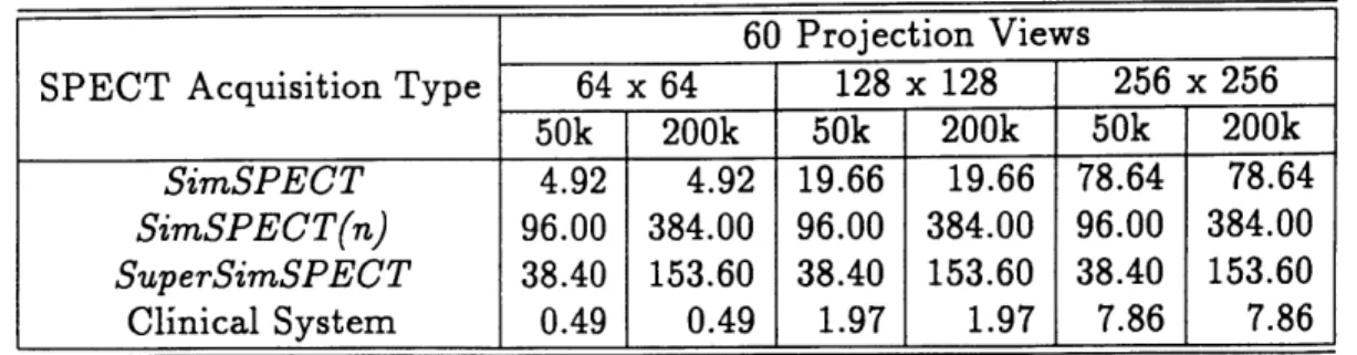
Table 2: SPECT data storage requirements for 60 tomograms at varying

res-olutions; total counts in each tomographic image are either 50,000 or 200,000,

as indicated (after energy selection). Sizes are in megabytes per study.

4

SimSPECT Performance

In this section, details are provided regarding the computational efficiency and

data storage requirements for the SimSPECT, SimSPECT(n), and

SuperSim-SPECT systems. A comparison is also made with selected other simulation

systems that model the acquisition of SPECT data.

4.1

Data Requirements

Storing synthetic SPECT data can require large amounts of space on magnetic

media such as hard disks. Table 2 indicates the megabyte amounts of space

required for various types of actual and simulated SPECT data.

Note that for the SimSPECT system, data are stored in pixel-based

Image-Mode files, whereas for SimSPECT(n) and SuperSimSPECT the data are

stored as lists of photons in ListMode files. For the clinical system, data

are stored in binary image files. As can be seen from the table, the storage

requirements for simulated SPECT data are significant, especially for

List-Mode data. However, the greater flexibility of ListList-Mode data more than

offsets these increased storage costs. Currently, we collect all simulation data

in ListMode format, and plan to continue this trend.

di

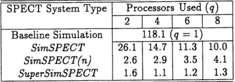
Table 3: SimSPECT run-times in linear CPU-days.

4.2

Time Requirements

Besides the fidelity of the simulated SPECT data and the ease with which software models can be prepared, the remaining important consideration in performing photon-level simulations of SPECT imaging systems is the compu-tational time required to generate adequate data and images. Table 3 presents a summary of the run-times for various SimSPECT systems and configura-tions. These data are calculated from the equations provided in Section 3, and for the SimSPECT and SimSPECT(n) systems, the agreement of the data with actual observed run-times is good; note that the SuperSimSPECT times are based on calculations only, as this system has not been completed to-date. The following parameters and normalizations have been used in calculating the run-times in Table 3. First, all values are for simulations that acquire 60 tomographic views. Second, the acceptance angle used results in an nff of 2. Third, the total number of disintegrations is 100 x 106 (resulting in approximately 10,000 counts per tomographic image within a +10% energy window. Fourth, all times are normalized to a machine with a MIPS CPU with a rating of 3.0 MFLOPS. Also, all run-times are given in linear CPU-days; to calculate total CPU-days (or the total amount of CPU time used), the data in the table should be multiplied by the number of processors used. As can be seen from Table 3, generating simulated SPECT images is compu-tationally expensive. Although these run-times appear formidable, the use of ListMode files imparts a degree of flexibility to the synthetic data such that many experiments can be performed using a single data set. Also, SimSPECT run-times are quite dependent on the type of patient or phantom model being used. For example, in an application where we simulated activity in small

SPECT System Type Processors Used (q)

2 4 6 8

Baseline Simulation 118.1 (q = 1) SimSPECT 26.1 14.7 11.3 10.0

SimSPECT(n)

2.6

2.9

3.5

4.1

lesions located on a rabbit aorta, 10, 000 counts in each tomographic view was more than adequate; however, for a large cylindrical water phantom filled with activity and containing several "cold" spheres with no activity, the number of counts per view for adequate 64 x 64 pixel images was over 300,000. These differences in minimal count levels are due to the differences in the volumes containing the activity. The larger the volume that contains a source material, the greater the number of photons that must be sampled and tracked from that volume in order to achieve acceptable photon statistics in each pixel.

4.3

Comparison with Related Systems

Numerous systems have been developed for simulating the acquisition of nu-clear medicine data. Numerical and analytical techniques have been tried, with analytical techniques requiring such severe restrictions on the problem formulation as to be essentially unusable for models requiring inhomogenous or asymmetric media. Numerical techniques, based predominantly on the use of Monte Carlo methods, have only recently progressed to the point of allowing fully 3-D, asymmetric models of source and transport objects to be used in conjuction with realistic models of collimators.

Examining only systems that allow realistic problems to be specified and then simulated (versus exhaustive collections of experimental data, or systems using constrained geometries), the hybrid approach of Kim et al [6] uses asymmetric models of source and transport objects. Although fast simulation times are achieved, this systems lacks the ability to model photon interactions within a collimator, and requires experimentally-derived data to simulate photon scat-ter as function of mascat-terial depth.

Zubal and Herrill [14] have built the most sophisticated system to-date, allow-ing asymmetric, 3-D models of patients to be used along with compton scatter interactions in the source objects. Advanced variance reduction methods are used to reduce simulation times, and an anatomically-correct, highly-detailed software patient phantom (acquired from CT studies) is used to generate sim-ulated SPECT data. Although data are provided only for the acquisition of planar images, and no details are given as to how tomographic images may be obtained, we estimate a production rate of approximately 1,000 detected pho-tons per tomgraphic view per CPU hour for the Zubal and Herrill system; this compares to the rate of 400 photons per hour per view for the SimSPECT(n)