The Connection Machine
by
William Daniel Hillis
M.S., B.S., Massachusetts Institute of Technology (1981, 1978)
Submitted to the Department of
Electrical Engineering and Computer Science in partial fulfillment of the
requirements for the degree of Doctor of Philosophy
at the
Massachusetts Institute of Technology June 1985
@W. Daniel Hillis, 1985
The author hereby grants to M.I.T. permission to reproduce and to distribute publicly copies of this thesis document in whole or in part.
Signature of Author. Department of Electrical Engineering and Computer Science May 3, 1985
Certified byG
Prc tsor Gerald Sussmnan, Thesis Supervisor
Acceptd by 'hairman, Ifepartment Committee
MASSACHUSETTS INSTiTUTE OF TECHNOL.OGY
The Connection Machine by
W. Daniel Hillis
Submitted to the Department of
Electrical Engineering and Computer Science
on May 3, 1985
in partial fulfillment of the requirements for the degree of
Doctor of Philosophy
Abstract
Someday, perhaps soon, we will build a machine that will be able to perform the functions of a human mind, a thinking machine. One of the many prob-lems that must be faced in designing such a machine is the need to process large amounts of information rapidly, more rapidly than is ever likely to be possible with a conventional computer. This document describes a new type of computing engine called a Connection Machine, which computes through the interaction of many, say a million, simple identical process-ing/memory cells. Because the processing takes place concurrently, the machine can be much faster than a traditional computer.
Thesis Supervisor: Professor Gerald Sussman
Contents
1 Introduction
1.1 We Would Like to Make a Thinking Machine
1.2 Classical Computer Architecture Reflects Obsolete Assumptions
Concurrency Offers a Solution ... 0. ... ....
Deducing the Requirements From an Algorithm The Connection Machine Architecture... Issues in Designing Parallel Machines... Comparison With Other Architectures... The Rest of the Story... Bibliographic Notes for Chapter 1.0... .. . a. 9. 0. 6. 1. 9. a. a. 0. 1. . 10 .. . a. 0. 0. 9. 9. 9. a. 0. 0. 9. 9. 15 21 . .. 25 28 30 31 2 How to Program a Connection Machine 2.1 Connection Machine Lisp Models the Connection Machine... 2.2 Alpha Notation... . ... 2.3 Beta Reduction... ... 2.4 Defining Data Structures with Defstruct (Background) .. R.. .. . .... 2.5 2.6 2.7 2.8 An Example: The Path-Length Algorithm... Generalized Beta (Optional Section)... CmLisp Defines the Connection Machine... . Bibliographic Notes for Chapter 2... . . . .a. .0... 33 33 38 42 42 .. . 1. . 44 46 48 . . .48 3 Design Considerations 50 3.1 The Optimal Size of a Processor/Memory Cell.. ... . 51
3.2 The Communications Network...8.9...54
3.3 Choosing a Topology... ... 55
3.4 Tour of the Topology Zoo...a.I... 56
3.5 Choosing A Routing Algorithm.... ... ... 59
3.6 Local versus Shared Control... ... ... 60
3.7 Fault Tolerance... ... 62
3.8 Input/Output and Secondary Storage.. ... 63
3.9 Synchronous versus Asynchronous Design... ... 64
3.10 Numeric versus Symbolic Processing ... ... ... 64
3.11 Scalability and Extendability .. op. .. .. . .. .. ... 65 1.3 1.4 1.5 1.6 1.7 1.8 1.9 6 6 9
3.12 Evaluating Success ... W... 3.13 Bibliographic Notes for Chapter 3...
Prototype The Chip...
The Processor Cell . . . . . The Topology. .I.. ... Routing Performance . . . . The Microcontroller . . . . Sample Operation: Addition
5 Data Structures for the Connection Mac
5.1 Active Data Structures ... ... ... 5.2 5.3 5.4 5.5 5.6 5.7 5.8 5.9 5.10 5.11 5.12 5.13 5.14 hine . . . . .l . . Sets ... ...
Bit Representation of Sets Tag Representation of Sets Pointer Representation of Sets Shared Subsets... Trees.4....0... Optimal Fanout of Tree Butterflies... Sorting On A Butterfly . . .0 Induced Trees... Strings...0... Arrays... Matrices... . ... 5.15 Graphs. . . ..
5.16 Bibliographic Notes for Chapt cr5 6 Storage Allocation and Defect
6.1 Free List Allocation...
6.2 Random Allocation0... 6.3 Rendezvous Allocation . . 6.4 Waves... 6.5 Block Allocation... .... 6.6 Garbage Collection..0.... 6.7 Compaction . . Tolerance . . . 1 . . . . .q . . . 111 111 113 114 115 117 118 . . . .a.I.a.0.a. . .120 4The 4.1 4.2 4.3 4.4 4.5 4.6 87 87 87 88 89 91 92 93 95 .100 101 102 104 105 107 108 110 66 68 69 70 71 75 80 84 85 . . .
6.8 Swapping ... .... .... ... .... .... a.. 122 6.9 Virtual Cells... ... 123 6.10 Bibliographic Notes for Chapter 6... . . . ... 124 7 New Computer Architectures and Their Relationship to Physics; or,
Why Computer Science is No Good 125
7.1 Connection Machine Physics...t...1..o.f...127
7.2 New Hope for a Science of Computation... . ... 129 7.3 Bibliographic Notes for Chapter 7...131
Chapter 1
Introduction
1.1
We Would Like to Make a Thinking Machine
Someday, perhaps soon, we will build a machine that will be able to perform the func-tions of a human mind, a thinking machine. One of the many problems that must be faced in designing such a machine is the need to process large amounts of information rapidly, more rapidly than is ever likely to be possible with a conventional computer. This document describes a new type of computing engine called a Connection Machine, which computes through the interaction of many, say a million, simple identical pro-cessing/memory cells. Because the processing takes place concurrently, the machine can be much faster than a traditional computer.
Our Current Machines Are Too Slow
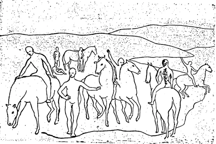
While the construction of an artificial intelligence is not yet within our reach, the ways in which current computer architectures fall short of the task are already evident. Consider a specific problem. Let us say that we are asked to describe, in a single sentence, the picture shown in Figure 1.1. With almost no apparent difficulty a person is able to say something like "It is a group of people and horses." This is easy for us. We do it almost effortlessly. Yet for a modern digital computer it is an almost impossible task. Given such an image, the computer would first have to process the hundreds of thousands of points of visual information in the picture to find the lines, the connected regions, the textures of the shadows. From these lines and regions it would then construct some sort of three-dimensional model of the shapes of the objects and
their locations in space. Then it would have to match these objects against a library of
known forms to recognize the faces, the hands, the folds of the hills, etc. Even this is not sufficient to make sense of the picture. Understanding the image requires a great deal of commonsense knowledge about the world. For example, to recognize the simple waving lines as hills, one needs to expect hills; to recognize the horses' tails, one needs to expect a tail at the end of a horse.
Even if the machine had this information stored in its memory, it would probably not find it without first considering and rejecting many other possibly relevant pieces
'p
' .
-~ -- r
of information, such as that people often sit on chairs, that horses can wear saddles, and that Picasso sometimes shows scenes from multiple perspectives. As it turns out, these facts are all irrelevant for the interpretation of this particular image, but the computer would have no a priori method of rejecting their relevance without considering them. Once the objects of the picture are recognized, the computer would then have to formulate a sentence which offered a concise description, This involves understanding which details are interesting and relevant and choosing a relevant point of view. For example, it would probably not be satisfactory to describe the picture as "Two hills, partially obscured by lifeforms," even though this may be accurate.
We know just enough about each of these tasks that we might plausibly undertake to program a computer to generate one-sentence descriptions of simple pictures, but the process would be tedious and the resulting program would be extremely slow. What the human mind does almost effortlessly would take the fastest existing computers many days. These electronic giants that so outmatch us in adding columns of numbers are equally outmatched by us in the processes of symbolic thought.
The Computer versus the Brain
So what's wrong with the computer? Part of the problem is that we do not yet fully understand the algorithms of thinking. But, part of the problem is speed. One might suspect that the reason the computer is slow is that its electronic components are much slower than the biological components of the brain, but this is not the case. A transistor can switch in a few nanoseconds, about a million times faster than the millisecond switching time of a neuron. A more plausible argument is that the brain has more neurons than the computer has transistors, but even this fails to explain the disparity in speed. As near as we can tell, the human brain has about 1010 neurons, each capable of switching no more than a thousand times a second. So the brain should be capable of about 1013 switching events per second. A modern digital computer, by contrast, may have as many as 109 transistors, each capable of switching as often as
1o9 times per second. So the total switching speed should be as high as 1018 events per
seconds, or
10,000
times greater than the brain. This argues the sheer computational power of the computer should be much greater than that of the human. Yet we know the reality to bejust
the reverse. Where did the calculation go wrong?1.2
Classical Computer Architecture Reflects Obsolete
As-sumptions
One reason that computers are slow is that their hardware is used extremely ineffi-ciently. The actual number of events per second in a large computer today is less than a tenth of one percent of the number calculated above. The reasons for the inefficiency are partly technical but mostly historical. The basic forms of today's architectures were developed tinder a very different set of technologies, when different assumptions applied than are appropriate today. The machine described here, the Connection Ma-chine, is an architecture that better fits today's technology and, we hope, better fits
the requirements of a thinking machine.
A modern large computer contains about one square meter of silicon. This square meter contains approximately one billion transistors which make up the processor and memory of the computer. The interesting point here is that both the processor and memory are made of the same stuff. This was not always the case. When von Neumann and his colleagues were designing the first computers, their processors were made of relatively fast and expensive switching components such as vacuum tubes, whereas the memories were made of relatively slow and inexpensive components such as delay lines or storage tubes. The result was a two-part design which kept the expensive vacuum tubes as busy as possible. This two-part design, with memory on one side and processing on the other, we call the von Neumann architecture, and it is the way that we build almost all computers today. This basic design has been so successful that most computer designers have kept it even though the technological reason for the memory/processor split no longer makes sense.
The Memory/Processor Split Leads to Inefficiency
In a large von Neumann computer almost none of its billion or so transistors are doing any useful process'ng at any given instant. Almost all of the transistors are in the
memory section of the machine, and only a few of those memory locations are being
accessed at any given time. The two-part architecture keeps the silicon devoted to processing wonderfully busy, but this is only two or three percent of the silicon area. The other 97 percent sits idle. At a million dollars per square meter for processed, packaged silicon, this is an expensive resource to waste. If we were to take another measure of cost in the computer, kilometers of wire, the results would be much the same: most of the hardware is in memory, so most of the hardware is doing nothing most of the time.
As we build larger computers the problem becomes even worse. It is relatively straightforward to increase the size of memory in a machine, it is far from obvious how to increase the size of the processor. The result is that as we build bigger machines with more silicon, or equivalently, as we squeeze more transistors into each unit of area, the machines have a larger ratio of memory to processing power and are consequently even less efficient. This inefficiency remains no matter how fast we make the processor because the length of the computation becomes dominated by the time required to move data between processor and memory. This is called the "von Neumann bottleneck." The bigger we build machines, the worse it gets.
1.3 Concurrency Offers a Solution
The obvious answer is to get rid of the von Neumann architecture and build a more homogeneous computing machine where memory and processing are combined. It is not difficult today to build a machine with hundreds of thousands or even millions of tiny processing cells which has a raw computational power that is many orders of magnitude greater than the fastest conventional machines. The problem lies in how to couple the raw power with the applications of interest, how to program the hardware to the job. How do we decompose our application into hundreds of thousands of parts that can be executed concurrently? How do we coordinate the activities of a million processing elements to accomplish a single task? The Connection Machine architecture was designed as an answer to these questions.
Why do we even believe that it is possible to perform these calculations with such a high degree of concurrency? There are two reasons. First, we have the existence proof of the human brain, which manages to achieve the performance we are after with a large number of apparently very slow switching components. Second, we have many specific examples in which particular computations can be achieved with high degrees of concurrency by arranging the processing elements to match the natural structure of the data.
Image Processing: One Processor per Pixel
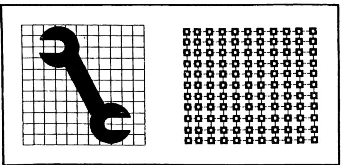
In image processing, for example, we know that it is possible to perform two-dimensional filtering operations efficiently using a two-dimensionally connected grid of processing elements. In this application it is most natural to store each point of the image in its own processing cell. A one thousand by one thousand point image would use a million processors. In this case, each step of the calculation can be performed
lo-Figure 1.2: In a machine vision application, a separate processor /memory cell processes each point in the image. Since the computation is two-dimensional the processors are connected into a two-dimensional grid.
cally within a pixel's processor or through direct communication with the processors' two-dimensionally connected neighbors. (See Figure 1.2.) A typical step of such a computation involves calculating for each point the average value of the points in the immediate neighborhood. Such averages can be computed simultaneously for all points in the image. For instance, to compute the average of each point's four immediate neighbors requires four concurrent processing steps during which each cell passes a value to the right, left, below, and above. On each of these steps the cell also receives a value from the opposite direction and adds it to its accumulated average. Four million
arithmetic operations are computed in the time normally required for four. VLSI Simulation: One Processor per Transistor
The image processing example works out nicely because the structure of the problem matches the communication structure of the cells. The application is two-dimensional, the hardware is two-dimensional. In other applications the natural structure of the problem is not nearly so regular and depends in detail on the data being operated
upon. An example of such an application outside the field of artificial intelligence is the simulation of an integrated circuit with hundreds of thousands of transistors.
Figure 1.3: In the VLSI simulation application a separate processor/memory cell is used to simulate each transistor. The processors are connected in the pattern of the circuit.
Such problems occur regularly in verifying the design of a very large scale integrated circuit. Obviously, the calculation can '>e done concurrently since the transistors do it concurrently, A hundred thousand transistors can be simulated by a hundred thousand processors. To do this efficiently, the processors would have to be wired into the same pattern as the transistors. (See Figure 1.3.) Each processor would simulate a single transistor by communicating directly with processors simulating connected transistors. When a voltage changes on the gate of a transistor the processor simulating the transistor calculates the transistor's response and communicates the change to processors simulating connected transistors. If many transistors are changing at once, then many responses are calculated concurrently, just as in the actual circuit. The natural connection pattern of the processors would depend on the exact connection pattern of the circuit being simulated.
Semantic Networks: One Processor per Concept
The human brain, as far as we know, is not particularly good at simulating transistors. But it does seem to be good at solving problems that require manipulating poorly struc-tured data. These manipulations can be performed by processors that are connected
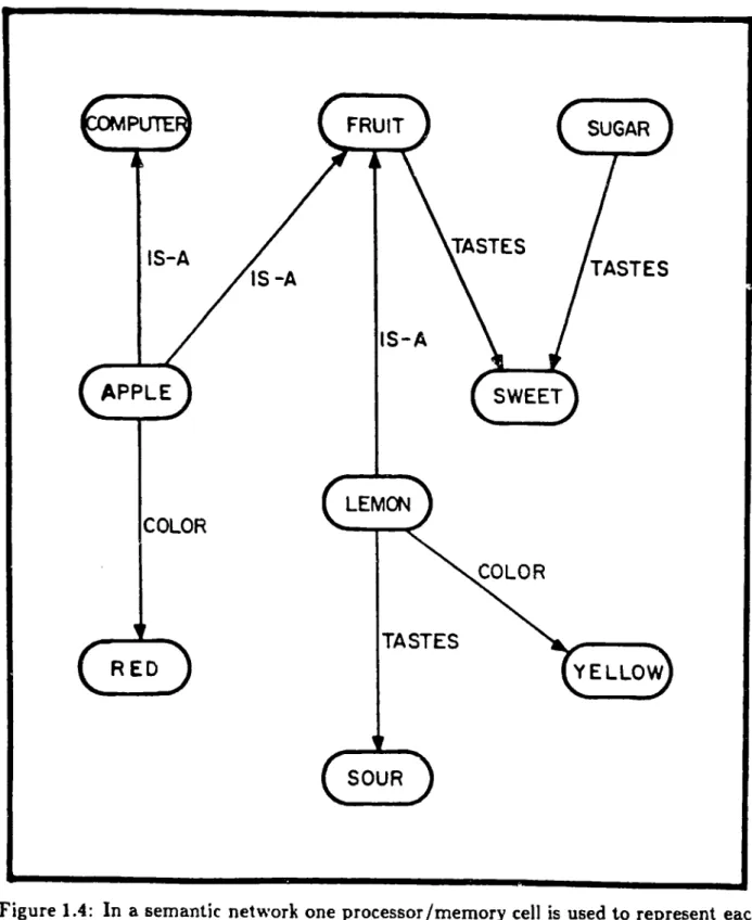
into patterns that mimic patterns of the data. For example, many artificial intelligence programs represent data in the form of semantic networks. A semantic network is a labeled graph where each vertex represents a concept and each edge represents a re-lationship between concepts. For example, Apple and Red would be represented by nodes with a Color-of link connecting between them. (See Figure 1.4.) Much of the knowledge that one might wish to extract from such a network is not represented ex-plicitly by the links, but instead must be inferred by:searching for patterns that involve multiple links. For example, if we know that My-Apple is an Apple, we may infer that My-Apple is Red from the combination of the Is-a link between My-Apple and Apple and the Color-of link between Apple and Red.
In a real-world database there are hundreds of thousands of concepts and millions of links. The inference rules are far more complex than simple Is-a deductions. For example, there are rules to handle exceptions, contradictions, and uncertainty. The system needs to represent and manipulate information about parts and wholes, spatial and temporal relationships, and causality. Such computations can become extremely complicated. Answering a simple commonsense question from such a database, such as
"Will my apple fall if I drop it?" can take a serial computer many hours. Yet a human answers questions such as this almost instantly, so we have good reason to believe that it can be done concurrently.
This particular application, retrieving commonsense knowledge from a semantic network, was one of the primary motivations for the design of the Connection Ma-chine. There are semantic network-based knowledge representation languages, such as NETL [Fahlman], which were specifically designed to allow the deductions necessary for retrieval to be computed in parallel. In such a system each concept or assertion can be represented by its own independent processing element. Since related concepts must communicate in order to perform deductions, the corresponding processors must be connected. In this case, the topology of the hardware depends on the information stored in the network. So, for example, if Apple and Red are related, then there must be a connection between the processor representing Apple and the processor repre-senting Red so that deductions about Apples can be related to deductions about Red. Given a collection of processors whose connection pattern matches the data stored in the network, the retrieval operations can be performed quickly and in parallel.
There are many more examples of this sort. For each, extreme concurrency can be achieved in the computation as long as the hardware is connected in such a way to match the particular structure of the application. They could each be solved quickly on a machine that provides a large number of processing memory elements whose connection
-A
ICOLOR
ACOLOR
Figure 1.4; In a semantic network one processor/memory cell is used to represent each concept and the connections between the cells represent the relationships between the concepts.
pattern can be reconfigured to match the natural structure of the application.
1.4
Deducing the Requirements From an Algorithm
We will consider a specific concurrent algorithm in detail and use it to focus on the architectural requirements for a parallel machine. Finding the shortest length path between two vertices in a large graph will serve as the example. The algorithm is
appropriate because, besides being simple and useful, it is similar in character to the many "spreading activation" computations in artificial intelligence. The problem to be solved is this:
Given a graph with vertices V and edges E C V x V, with an arbitrary
pair of vertices a, b E V, find the length k of shortest sequence of connected
vertices a,v1,v27,...b such that all the edges (a,vx),(vI,v2), ... (vk - 1, b) E E
are in the graph.
For concreteness, consider a graph with 10 vertices and an average of 102 randomly connected edges per vertex. (For examples of where such graphs might arise, see [Quillian],
[Collins,
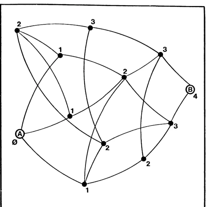
Loftus], [Waltz]). In such a graph, almost any randomly chosen pair of vertices will be connected by a path of not more than three edges.The algorithm for finding the shortest path from vertex A to vertex B begins by labeling every vertex with its distance from A. This is accomplished by labeling vertex
A with 0, labeling all vertices connected to A with 1, labeling all unlabeled vertices
connected to those vertices with 2, and so on. (See Figure 1.5.) The process terminates as soon as vertex B is labeled, The label of B is then the length of the shortest connecting path. Any path with monotonically decreasing labels originating from B will lead to A in ths number of steps. A common optimization of this algorithm is to propagate the labels from A and B simultaneously until they meet, but for the sake of clarity we will stick to its simplest form.
Ideally we would be able to describe the algorithm to the computer something like this:
Algorithm I: "Finding the length of shortest path from A to B"
1. Label all vertices with
+joo.
2. Label vertex A with 0,3. Label every vertex, except A, with 1 plus the minimum of its neighbor's labels and itself. Repeat this step until the label of vertex B is finite.
3
W4
Figure 1.5: Algorithm I finds the length of the shortest path from vertex A to vertex B by labeling each point with its distance from A.
4. Terminate. The label of B is the answer.
We will use this path-length algorithm as an example to motivate the structure of the Connection Machine.
Algorithms of this type are slow on a conventional computer. Assuming that each step written above takes unit time, Algorithm I will terminate in time proportional to the length of the connecting path. For the 104 vertex random graph mentioned above,
Step 3 will be repeated two or three times, so about six steps will be required to find the path length. Unfortunately, the steps given above do not correspond well with the kinds of steps that can be executed on a von Neumann machine. Direct translation of the algorithm into Lisp gives this a very inefficient program. The program runs in time proportional to the number of vertices, times the length of the path, times the average degree of each vertex. For example, the graph mentioned above would require several million executions of the inner loop. Finding a path in a test graph required about an hour of CPU time on a VAX-11/750 computer.
Besides being slow, a serial program would implement the dissimilar operations with similar constructs, resulting in a more obscure rendition of the original algorithm. For example, in the algorithm, iteration is used only to specify multiple operations that need to take place in time-sequential order, which is where the sequencing is critical to the algorithm. In a serial program everything must take place in sequence. The iteration would be used not only to do things that are rightfully sequential, but also to operate all of the elements of a set and to find the minimum of a set of numbers.
A good programmer could, of course, change the algorithm to one that would run faster. For example, it is not necessary to propagate labels from every labeled vertex, but only from those that have just changed. There are also many well-studied opti-mizations for particular types of graphs. We have become so accustomed to making such modifications that we tend to make them without even noticing. Most program-mers given the task of implementing Algorithm I probably would include several such optimizations almost automatically. Of course, many "optimizations" would help for some graphs and hurt for others. For instance, in a fully connected graph the extra overhead of checking if a vertex had just changed would slow things down. Also, with optimizations it becomes more difficult to understand what is going on. Optimization
trades speed for clarity and flexibility.
Instead of optimizing the algorithm to match the operation of the von Neumann machine, we could make a machine to match the algorithm. Implementing Algorithm I directly will lead us to the architecture of the Connection Machine.
Requirement 1: Many Processors
To implement the path-length algorithm directly, we need concurrency. As Algorithm I is described, there are steps when all the vertices change to a computed value simul-taneously. To make these changes all at once, there must be a processing element associated with each vertex. Since the graph can have an arbitrarily large number of vertices, the machine needs an arbitrarily large number of processing elements. Un-fortunately, while it is fine to demand infinite resources, any physical machine will be only finite. What compromise should we be willing to make?
It would suffice to have a machine with enough processors to deal with most of the problems that arise. How big a machine this is depends on the problems. It will be a tradeoff between cost and functionality.
We are already accustomed to making this kind of tradeoff for the amount of memory on a computer. Any real memory is finite, but it is practical to make the memory large enough that our models of the machine can safely ignore the limitations. We should be willing to accept similar limitations on the number of processors. Of course, as with memory, there will always be applications where we have to face the fact of finiteness. In a von Neumann machine we generally assume that the memory is large enough to hold the data to be operated on plus a reasonable amount of working storage, say in proportion to the size of the problem. For the shortest path problem we will make similar assumptions about the availability of processors. This will -be the first design requirement for the machine, that there are enough processing elements to be allocated as needed, in proportion to the size of the problem.
A corollary of this requirement is that each processing element must be as small and as simple as possible so that we can afford to have as many of them as we want. In particular, it can only have a very small amount of memory. This is an important design constraint, It will limit what we can expect to do within a single processing element. It would not be reasonable to assume both "there are plenty of processors" and "there is plenty of memory per processor." If the machine is to be built, it must use roughly the same number of components as conventional machines. Modern production technology gives us one "infinity" by allowing inexpensive replication of components. It is not fair to ask for two.
Requirement II: Programmable Connections
In the path-length algorithm, the pattern of inter-element communication depends on the structure of the graph. The machine must work for arbitrary graphs, so every
processing element must have the potential of communicating with every other pro-cessing element. The pattern of connections must be a part of the changeable state of the machine. (In other problems we will actually want to change the connections dynamically during the course of the computation, but this is not necessary for the path-length calculation.)
From the standpoint of the software the connections must be programmable, but the processors may have a fixed physical wiring scheme. Here again there is an analogy with memory. In a conventional computer the storage elements for memory locations 4 and 5 are located in close physical proximity, whereas location 1000 may be physically on the other side of the machine, but to the software they are all equally easy to access. If the machine has virtual memory, location 1000 may be out on a disk and may require much more time to access. From the software this is invisible. It is no more difficult to move an item from location 4 to 1000 than it is from 4 to 5. We would like a machine that hides the physical connectivity of the processors as thoroughly as the von Neumann computer hides the physical locality of its memory. This is an important part of molding the structure of our machine to the structure of the problem. It forms the second requirement for the machine, that the processing elements are connected by software.
This ability to configure the topology of the machine to match the topology of the problem will turn out to be one of the most important features of the Connection Machine. (That is why it is called a Connection Machine.) It is also the feature that presents the greatest technical difficulties. To visualize how such a communications network might work, imagine that each processing element is connected to its own message router and that the message routers are arranged like the crosspoints of a grid, each physically connected to its four immediate neighbors (Figure 1.6). Assume that one processing element needs to communicate with another one that is, say, 2 up and 3 to the right. It passes a message to its router which contains the information to be transmitted plus a label specifying that it is to be sent 2 up and 3 over. On the basis of that label, the router sends the message to its neighbor on the right, modifying the label to say "2 up and 2 over." That processor then forwards the message again, and so on, until the label reads "0 up and 0 over." At that point the router receiving the message delivers it to the connected processing element.
In practice, a grid is not really a very good way to connect the routers because routers can be separated by as many as 2(g'n) intermediaries, It is desirable to use much more complicated physical connection schemes with lots of short-cuts so that the maximum distance between any two cells is very small. We also need to select the
Figure 1.6: A simple (but inefficient) communications network topology
routing algorithms carefully to avoid "traffic jams" when many messages are traveling through the network at once. These problems are discussed in detail in Chapter 4. The important thing here is that processing elements communicate by sending mes-sages through routers. Only the routers need to worry about the physical connection topology. As long as two processing elements know each other's address, they can communicate as if they were physically connected. We say there is a virtual connection
between them, The virtual connection presents a consistent interface between proces-sors. Since the implementation details are invisible, the software can remain the same
as technology changes, wires break, and hardware designers think of new tricks.
In the path-length algorithm, a vertex must communicate with all of its neighbors. The fanout of the communication is equal to the number of neighbors of the vertex. Since a vertex may have an arbitrary number of connected edges, the fanout of a processing element must be unlimited. Similarly, a vertex may receive communication from an arbitrarily large number of edges simultaneously. A processing element must be able to send to and receive from an arbitrary number of others.
Does this mean that each processing element must be large enough to handle many messages at once? Will it need arbitrary amounts of storage to remember all of its connections? Providing large amounts of storage would contradict the need to keep the
Trees Allow Arbitrary Fanout
The term "fanout tree" comes from electrical engineering. A related fanout problem comes up electrically because it is impossible to measure a signal without disturbing it. This sounds like a mere principle of physics, but every engineer knows its macroscopic consequences. In standard digital electronics, for instance, no gate can directly drive more than about ten others. If it is necessary to drive more than this then it can be accomplished by a tree of buffers. One gate drives ten buffers, each of which drive ten more, and so on, until the desired fanout is achieved. This is called a fanout tree.
There is a software equivalent to this in languages like Lisp, where large data struc-tures are built out of small, fixed-sized components. The Lisp "cons cell" has room for only two pointers. Sequences of arbitrary many elements are represented by stringing together multiple cons cells. Lisp programmers use linear lists more often than trees, because they are better suited for sequential access. Balanced trees are used when the time to access an arbitrary element is important.
The use of trees to represent a network with fanout is illustrated in Figure 1.7. No-tice that each node is connected to no more than three others. (Lisp gets away with two because the connections are not bidirectional, so it does not store the "backpointers.") Since a balanced tree with N leaves requires 2N - 1 nodes, the number of 3-connected processing elements required to represent any graph is equal to twice the number of edges minus the number of vertices. The tree structure "wastes" memory by storing the internal structure of the tree, just as the Lisp list "wastes" a factor of two in storage oy storing the links from one node to the next. But because each vertex of the graph is represented by a tree of processing elements rather than by a single processing element, there is storage and processing power at each vertex in proportion to the number of connected edges. This solves the problem of how to handle multiple messages arriving
at once. Each processing element only needs to handle a maximum of three messages. It also keeps the elements small since each needs only the addresses that correspond to three virtual connections. There is a cost in time: a vertex must communicate data through its internal tree before the data can be communicated out to the connected vertices. This internal communication requires O(log V) message transmission steps, where V is the degree of the vertex.
1.5 The Connection Machine Architecture
in the preceding sections we have identified two requirementz for a machine to solve the path-length problem:
Representation cf
A Simple Virtual Copy Network
IS-A
LEMON SOUR
Figure 1.7: Use of trees to represent a network with fanout (this is the representation of the semantic network shown in Figure 1,4)
* Requirement I: There are enough processing elements to be allocated as needed, in proportion to the size of the problem.
* Requirement II: The processing elements can be connected by software.
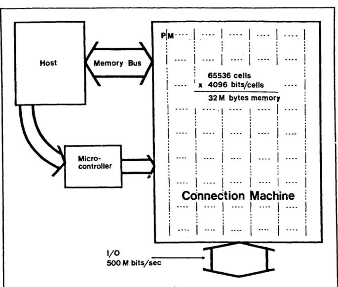
The Connection Machine architecture follows directly from these two requirements. It provides a very large number of tiny processor/memory cells, connected by a pro-grammable communications network. Each cell is sufficiently small that it is incapable of performing meaningful computation on its own. Instead multiple cells are connected together into data-dependent patterns called active data structures which both repre-sent and process the data. The activities of these active data structures are directed from outside the Connection Machine by a conventional host computer. This host com-puter stores data structures on the Connection Machine in much the same way that a conventional machine would store them in a memory. Unlike a conventional memory, though, the Connection Machines has no processor/memory bottleneck. The memory cells themselves do the processing. More precisely, the computation takes place through the coordinatea interaction of the cells in the data structure. Because thousands or even millions of processing cells work on the problem simultaneously, the computation proceeds much more rapidly than would be possible on a conventional machine.
A Connection Machine connects to a conventional computer much like a conven-tional memory. Its internal state can be read and written a word at a time from the conventional machine. It differs from a conventional memory in three respects. First, associated with each cell of storage is a processing cell which can perform local com-putations based on the information stored in that cell. Second, there exists a general intercommunications network that can connect all the cells in an arbitrary pattern, Third, there is a high-bandwidth input/output channel that can transfer data between the Connection Machine and peripheral devices at a much higher rate than would be possible through the host.
A connection is formed from one processing memory cell to another by storing a
pointer in the memory. These connections may be set up by the host, loaded through
the input/output channel, or determined dynamically by the Connection Machine itself. In the prototype machine described in Chapter 4, there are 65,536 processor
/memory
cells, each with 4,096 bits of memory. This is a small Connection Machine. The block diagram of the Connection Machine with hosts, processoi /memory cells, communica-tions network, and input/output is as shown in Figure 1.8.
The control of the individual processor/memory cells is orchestrated by the host of the computer. For example, the host may ask each cell that is in a certain state
Host Memory Bus 65536 cells - --- x 4096 bits/cells --32 M bytes memory Micro- ----
---
----
---- ----controllerConnection Machine
1/0 500 M bits/secto add two of its memory locations locally and pass the resulting sum to a connected cell through the communications network. Thus, a single command from the host may result in tens of thousands of additions and a permutation of data that depends on the pattern of connections. Each processor/memory cell is so small that it is essentially incapable of computing or even storing any significant computation on its own. Instead, computation takes places in the orchestrated interaction of thousands of cells through
the communications network.
1.6
Issues in Designing Parallel Machines
The remainder of the thesis is devoted primarily to the dual questions of how to use the architecture to solve problems and how to implement the architecture in terms of available technology. In other words, how do we program it, and how do we build it? First we must establish that we are programming and building the right thing, Parallel processing is inevitable. But what form will it take? So little is known about parallel computation that informed intelligent architects will make very different decisions when confronted with the same set of choices. This section will outline three of the most important choices in designing any parallel machine:
* General versus fixed communication; " Fine versus coarse granularity; and
* Multiple versus single instruction streams.
Although each issue may be characterized by the extreme schools of thought, each offers a spectrum of choices, rather than a binary decision. Each choice is relatively independent, so in principle there is a different type of computer architecture for each combination of choices.
Fixed versus General Communication
Some portion of the computation in all parallel machines involves communication among the individual processing elements. In some machines, such communication is allowed in only a few specific patterns defined by the hardware. For example, the processors may be arranged in a two-dimensional grid, with each processor cornnected to its north, south, east, and west neighbors. A single operation on such a machine could send a number from each processor to its northern neighbor, Proposed con-nection patterns for such fixed-topology machines include rings, n-dimensional cubes,
and binary trees. The alternative to a fixed topology is a general communications network that permits any processor to communicate with any other. An extreme ex-ample of an architecture with such a general communications scheme is the hypothetical "para-computer," [Schwartz, 1980] in which every processor can simultaneously access a common shared memory. In a para-computer, any two processors can communicate by referencing the same memory location.
Depending on how a general communications network is implemented, some pairs of processors may be able to communicate more quickly than others, since even in general communications schemes the network has an underlying unchanging physical pattern of wires and cables, which can be visible to the programmer in different degrees. At the other extreme, a fixed-topology machine may be programmed to emulate a general machine with varying difficulty and efficiency.
The primary advantage of fixed-topology machines is simplicity. For problems where the hardwired pattern is well matched to the application, the fixed-topology machines can be faster. Examples of such matches are the use of a two-dimensional grid pattern for image processing, and a shuffle-exchange pattern for Fast Fourier Transforms. The general communications machines have the potential of being fast and easier to program for a wider range of problems, particularly those that have less structured patterns of communication. Another potential advantage is that the connection pattern can change dynamically to optimize for particular data sets, or to bypass faulty components.
Coarse-Grained versus Fine-Grained
In any parallel computer with multiple processing elements, there is a trade-off between the number and the size of the processors. The conservative approach uses as few as possible of the largest available processors. The conventional single processor von Neumann machine is the extreme case of this. The opposite approach achieves as much parallelism as possible by using a very large number of very small machines. We can characterize machines with tens or hundreds of relatively large processors as
"coarse-grained" and machines with tens of thousands to millions of small processors
as "fine-grained." There are also many intermediate possibilities.
The fine-grained processors have the potential of being faster because of the larger degree of parallelism. But more parallelism does not necessarily mean greater speed. The individual processors in the small-grained design are necessarily less powerful, so many small processors may be slower than one large one. For almost any application there are at least some portions of the code that run most efficiently on a single pro-cessor. For this reason, fine-grained architectures are usually designed to be used in
conjunction with a conventional single-processor host computer.
Perhaps the most important issue here is one of programming style. Since serial
processor machines are coarse-grained, the technology for programming coarse-grained machines is better understood. It is plausible to expect a Fortran compiler to optimize code for, say, sixteen processing units, but not for sixteen thousand. On the other hand, if the algorithm is written with parallel processing in mind from the start, it may be that it divides naturally into the processors, of a fine-grained machines. For example, in a vision application it may be most natural to specify a local algorithm to be performed on each point in an image, so a 1000 x 1000 image would most naturally fit onto a million processor machine.
Single versus Multiple Instruction Streams
A Multiple Instruction Multiple Data (MIMD) machine is a collection of connected autonomous computers, each capable of executing its own program. Usually a MIMD machine will also include mechanisms for synchronizing operations between processors when desired. In a Single Instruction Multiple Data (SIMD) machine, all processors are controlled from a single instruction stream which is broadcast to all the processing elements simultaneously, Each processor typically has the option of executing an in-struction or ignoring it, depending on the processor's internal state. Thus, while every processing element does not necessarily execute the same sequence of instructions, each processor is presented with the same sequence. Processors not executing must "wait out" while the active processors execute.
Although SIMD machines have only one instruction stream, they differ from MIMD machines by no more that a multiplicative constant in speed. A SIMD machine can simulate a MIMD machine in linear time by executing an interpreter which interprets each processor's data as instructions. Similarly, a MIMD machine can simulate a SIMD. Such a simulation of a MIMD machine with a SIMD machine (or vice versa) may or may not be a desirable thing to do, but the possibility at least reduces the question
from one of philosophy to one of engineering: Since both types of machines can do the
same thing, which can do it faster or with less hardware?
The correct choice may depend on the application. For well-structured problems with regular patterns of control, SLMD machines have the edge, because more of the hardware is devoted to operations on the data, This is because the SIMD machine, with only one instruction stream, car share most of its control hardware among all processors. In applications where the control flow required of each processing element is complex and data-dependent, MIMD architecture may have an advantage. The
shared instruction stream can follow only one branch of the code at a time, so each possible branch must be executed in sequence, while the uninterested processor is idle. The result is that processors in a SIMD machine may sit idle much of the time.
The other issue in choosing between a SIMD and a MIMD architecture is one of programmability. Here there are arguments on both sides. The SIMD machine eliminates problems of synchronization. On the other hand, it does so by taking away the possibility of operating asynchronousiy. Since either type of machine can efficiently emulate the other, it may be derirable to choose one style for programming and the other for hardware.
Gordon Bell [BellJ has characterized SIMD and MIMD machines as having differ-ent characteristic "synchronization times" and has pointed out that differdiffer-ent MIMD machines have different characteristic times between processor synchronization steps varying from every few instructions to entire tasks. There are also SIMD machines that allow varying amounts of autonomy for the individual processing elements and/or several instruction streams, so once again this issue presents a spectrum of possible choices.
1.7
Comparison With Other Architectures
Different architectures make different choices with respect to the key decisions outlined above. In this section, we contrast the Connection Machine architecture with some other approaches to building very high performance computers. The most important distinguishing feature of the Connection Machine is the combination of fine granularity and general communication. The Connection Machine has a very large number of very small processors. This provides a high degree of parallelism and helps solve resource-allocation problems. Also, the communications network allows the connectivity of these processors to be reconfigured to match a problem. This ability to "wire up" thousands of programmable processing units is really the heart of the Connection Machine con-cept. Below we summarize some of the approaches taken by other architectures. For references to specific examples see the bibliographic notes at the end of the chapter.
Fast von Neumann Machines
There are a large number of ongoing efforts to push the performance of conventional serial machines. These involve the use of faster switching devices, the use of larger and more powerful instruction sets, the use of smaller and simpler instruction sets, improvements in packaging, and tailoring the machines to specific applications. Even
if the most exotic of these projects are completely successful, they will not come close
to meeting our performance requirements. When performing simple computations on
large amounts of data, von Neumann computers are limited by the bandwidth between memory and processor. This is a fundamental flaw in the von Neumann design; it cannot be eliminated by clever engineering.
Networks of Conventional Machines
Other researchers have proposed connecting dozens or even hundreds of conventional computers by shared memory or a high bandwidth communications network. Several of these architectures are good candidates for machines with orders of magnitude in increased performance. Compared to the Connection Machine, these architectures have a relatively small number of relatively large machines. These machines have a much lower ratio of processing power to memory size, so they are fundamentally slower than the Connection Machine on memory intensive operations.
Machines with Fixed Topologies
Much closer to the Connection Machine in the degree of potential parallelism are the tessellated or recursive structures of many small machines. The most common topolo-gies are the two-dimensional grid or torus. These machines have fixed interconnection topologies, and their programs are written to take advantage of the topology. When the structure of the problem matches the structure of the machine, these architectures can exhibit the same or higher degree of concurrency as the Connection Machine, Unlike the Connection Machine, their topologies cannot be reconfigured to match a particu-lar problem. This is particuparticu-larly important in problems such as logic simulation and semantic network inference, for which the topology is highly irregular.
Database Processors
There have been several special-purpose architectures proposed for speeding up database
search operations. Like the Connection Machine, these database processors are de-signed to perform data-intensive operations under control of a more conventional host computer. Although these machines are designed to process a restricted class of queries on larger databases, they have many implementation issues in common with the Con-nection Machine. The study of these architectures has produced a significant body of theory on the computational complexity of parallel database operations.
Marker Propagation Machines
The Connection Machine architecture was originally developed to implement the marker-propagation programs for retrieving data from semantic networks [Fahlman, 1979). The Connection Machine is well suited for executing marker-type algorithms, but it is considerably more flexible than special-purpose marker propagators. The Connec-tion Machine has a computer at each node which can manipulate address pointers and send arbitrary messages, It has the capability to build structures dynamically. These features are important for applications other than marker-passing.
Cellular Automata and Systolic Arrays
A systolic array is a tessellated structure of synchronous cells that perform fixed se-quences of computations with fixed patterns of communication. In the Connection Machine, by contrast, both computations and the communications patterns are
pro-grammable. In the Connection Machine, uniformity is not critical. Some cells may be defective or missing. Another structure, similar to the systolic array, are cellular automata. In an abstract sense, the Connection Machine is a universal cellular au-tomaton, with art additional mechanism added for non-local communication. In other words, the Connection Machine hardware hides the details. This additional mechanism makes a large difference in performance and ease of programming.
Content Addressable Memories
The Connection Machine may be used as a content addressable or associative memory, but it is also able to perform non-local computations through the communications network. The elements in content addressable memories are comparable in size to connection memory cells, but they are not generally programmable. When used as a content addressable memory, the Connection Machine processors allow more complex matching procedures.
1.8
The Rest of the Story
The remainder of this document discusses in detail how to program and build Con-nection Machines. Chapter 2 describes a programming language based on Lisp which provides an idealized model of what a Connection Machine should do in the same sense that a conventional programming language provides an idealized model of a conven-tional machine. Chapter 3 discusses some of the issues that arise in implementing the
architecture and hardware. Chapter 4 describes the details of an actual prototype. Chapter 5 is a discussion of active data structures and ;D description of some of the fundamental algorithms for the Connection Machine. Chapter 6, on storage allocation, shows how these data structures can be built and transformed dynamically. It also discusses the related issue of why a Connection Machine can work even when some of its components do not. The final chapter, Chapter 7, is a philosophical discussion of computer architecture and what the science of computation may look like in the future, Most of the references to related works have been moved out of the text and into the Bibliographic Notes at the end of each chapter. There is also an annotated bibliography at the end of the document which gives for each reference some justification of why it might be worth reading in this context.
1.9
Bibliographic Notes for Chapter 1
The quest to make a thinking machine is not new. The first reference of which I am aware in the literature is in The Politic
[Aristotle],
where Aristotle speaks of au-tonomous machines that can understand the needs of their masters as an alternative to slavery. For centuries this remained only a dream, until the 1940's, when an increased understanding of servo-mechanisms led to the establishment of the field of cybernetics [Wiener, 1948],[Ashby,
1956). Cybernetic systems were largely analog. Soon after-ward the development of digital computing machinery gave rise to comparisons with the symbolic functions of the mind [Turing, 1950], [von Neumann, 1945], which led, in the early 1960's, to the development of the field of artificial intelligence [Minsky, 1961),[Newell, 1963]. For a very readable history of these developments see
[Boden,
1977]. For insight to the motivation of the two-part von Neumann design (including some amusing predictions of things like potential applications and memory sizes), I suggest reading some of the original documents [Burks, 1946-1957),|Goldstein,
1948],[von
Neumann, 1945). For a good ,.ief introduction to semantic networks see [Woods, 1975). For examples of specific semantic network representation schemes see (Brachman, 1978],
[Fahlman,
1979],[Hewitt,
1980],[Shapiro,
1976],[Szolovitz,
1977], and in particular forsemantic networks designed to be accessed by parallel algorithms see IQuillian, 1968], [Fahlman, 1979],
[Woods,
19781. For discussions of the semantics of semantic networkssee
[Brachman,
1978],[Hendrix,
1975],[Woods,
1975]. There are many other knowledgerepresentation schemes in artificial intelligence that were designed with parallelism in mind, for example, "connectionist" theories
[Feldman,
1981], k-lines[Minsky,
1979], word-expert parsing[Small,
1980), massively parallel parsing[Waltz,
1985], and schemamechanisms [Drescher, 1985], classifier systems
[Holland,
19591. It may also be that parallelism is applicable to the access of the highly-structured knowledge in expert systems [Stefik, 1982]. One of the most exciting potential'application areas of the machine is in systems that actually learn from experience. Such applications would be able to use to advantage the Connection Machine's ability to dynamically change its own connections. For examples of recent approaches to learning see[Winston,
19801, [Hopfield, 1982), [Minsky, 1982).For a recent survey of parallel computing see [Haynes, 1982] and
[Bell,
1985]. My discussion of the issues in this chapter follows the taxonomy introduced in [Schwartz, 1983]. For a fun-to-read paper on the need for raw power and parallelism see[Moravec,
1979]. The phrase "von Neumann bottleneck" comes from Backus's Turing Lecture [Backus, 1978], in which he eloquently sounds the battle cry against word-at-a-time thought.For examples of alternative parallel architectures the reader is referred to the anno-tated bibliography at the end of the thesis. The references therein may be divided as follows. Large- to medium-grain machines: [Bell, 1985], |Bouknight, 1972],
[Buehrer,
1982), [Chakravarthy, 1982), [Davidson, 1980, [Gajski, 1983],[Gottlieb,
1982, 1983, [Halstead, 1978, 1979, 1980, [Hewitt, 1980, [Keller, 1978, 1979],[Kuch,
1982],[Lund-strom, 1980], [Rieger, 1979, 1980, [Schwartz, 1980, [Shin, 1982], [Slotnick, 1978, [Stolfo, 1982], [Sullivan, 1977], [Swan, 1977], [Treleaven, 1980], [Trujillo, 1982], [Ward, 1978], [Widdoes, 1980). Small-grain machines: [Batcher, 1974, 1980],
[Browning,
1980],
[Burkley,
1982), [Carroll, 1980), [DiGiacinto, 1981],[Fahlman,
1981), [Gilmore, 1982], [Gritton, 1977], [Holland, 1959, 1960, [Lee, 1962, [Mago, 1979, [Schaefer, 1982], [Shaw, 1982], [Snyder, 1982], [Surprise, 1981]. Database machines: [Copeland, 1973], [Hawthorn, 1982], [Kung, 1980, [Ozkarahan, 1974. Data flow:[Arvind,
1978, 1983], [Dennis, 1977, 1980]. Special purpose machines:|Chang,
1978],[Forster,
1982], [Hawkins, 1963], [Kung, 1980], [Lipovski, 1978], [Meadows, 1974], [Parhami, 1972], [Reeves, 1981], [Siegel, 1981]. Content addressable memories: [Lee, 1962, 1963).For some comparisons of the performance of various machines see [Dongarra, 1984],
[Tenenbaum,
1983], and[Hawthorn,
1982]. Not all computations can be speeded up byChapter 2
How to Program a Connection Machine
2.1
Connection Machine Lisp Models the Connection Machine
It is easy to forget how closely conventional languages correspond to the hardware of a conventional computer, even for "high-level" languages like Lisp. The control flow in Lisp, for example, is essentially an abstract version of the hardware instruction fetching mechanism of a serial machine. Objects are pointers, CAR and CDR are indirect address-ing. Function invocation is a subroutine call. Assignment is storing into memory. This close correspondence between Lisp and the machine on which it is implemented accounts for much of the language's power and popularity. It makes it easy to write compilers. It makes the language easier to think about and, more important, it allows the performance of algorithms to be compared and estimated without reference to the details of a particular machine. The language captures what is common and essential to a wide range of serial computers, while hiding the details that set them apart.Connection Machine Lisp (CmLisp) is an extension of Common Lisp, designed to support the parallel operations of the Connection Machine. It is intended to be for the Connection Machine architecture what Lisp is for the serial computer: an expression of the essential character of the architecture that leaves out the details of implementation. In the sense that Fortran or Lisp are abstract versions of a conventional computer, Cm-Lisp is an abstract version of the Connection Machine. Just as these languages hide such details of the computer as word length, instruction set, and low-level storage con-ventions, CmLisp hides the details of the Connection Machine. Just as conventional languages reflect the architecture of conventional computers, CmLisp reflects the
archi-tecture of the Connection Machine. The structure of the language follows the structure
of the hardware.
An example of this correspondence is the relatively conventional control structure of Cmbisp, which is very similar to languages like FP and APL. in CmLisp, as in the Connection Machine itself, parallelism is achieved through simultaneous operations over composite data structures rather than through concurrent control structures. in this sense Cmbisp is a relatively conservative parallel language, since it retains the program flow and control constructs of a normal serial Lisp, but allows operations to