HAL Id: lirmm-01402222
https://hal-lirmm.ccsd.cnrs.fr/lirmm-01402222
Submitted on 24 Nov 2016
HAL is a multi-disciplinary open access archive for the deposit and dissemination of sci-entific research documents, whether they are pub-lished or not. The documents may come from teaching and research institutions in France or abroad, or from public or private research centers.
L’archive ouverte pluridisciplinaire HAL, est destinée au dépôt et à la diffusion de documents scientifiques de niveau recherche, publiés ou non, émanant des établissements d’enseignement et de recherche français ou étrangers, des laboratoires publics ou privés.
NIRS-EEG joint imaging during transcranial direct
current stimulation: online parameter estimation with
an autoregressive model
Mehak Sood, Pierre Besson, Makii Muthalib, Utkarsh Jindal, Stéphane
Perrey, Anirban Dutta, Mitsuhiro Hayashibe
To cite this version:
Mehak Sood, Pierre Besson, Makii Muthalib, Utkarsh Jindal, Stéphane Perrey, et al..
NIRS-EEG joint imaging during transcranial direct current stimulation: online parameter estimation
with an autoregressive model. Journal of Neuroscience Methods, Elsevier, 2016, 274, pp.71-80.
Accepted Manuscript
Title: NIRS-EEG joint imaging during transcranial direct current stimulation: online parameter estimation with an autoregressive model
Author: Mehak Sood Pierre Besson Makii Muthalib Utkarsh Jindal Stephane Perrey Anirban Dutta Mitsuhiro Hayashibe
PII: S0165-0270(16)30216-3
DOI: http://dx.doi.org/doi:10.1016/j.jneumeth.2016.09.008 Reference: NSM 7597
To appear in: Journal of Neuroscience Methods
Received date: 13-3-2016 Revised date: 24-9-2016 Accepted date: 26-9-2016
Please cite this article as: Sood Mehak, Besson Pierre, Muthalib Makii, Jindal Utkarsh, Perrey Stephane, Dutta Anirban, Hayashibe Mitsuhiro.NIRS-EEG joint imaging during transcranial direct current stimulation: online parameter estimation with an autoregressive model.Journal of Neuroscience Methods http://dx.doi.org/10.1016/j.jneumeth.2016.09.008
This is a PDF file of an unedited manuscript that has been accepted for publication. As a service to our customers we are providing this early version of the manuscript. The manuscript will undergo copyediting, typesetting, and review of the resulting proof before it is published in its final form. Please note that during the production process errors may be discovered which could affect the content, and all legal disclaimers that apply to the journal pertain.
NIRS-EEG joint imaging during transcranial direct current stimulation:
online
parameter
estimation
with
an
autoregressive
model
Mehak Sood# (Author)
Electronics and Communication Engineering International Institute of Information Technology Hyderabad, India
Pierre Besson# (Author) EUROMOV
Université de Montpellier Montpellier, France
Makii Muthalib (Author)
EUROMOV
Université de Montpellier Montpellier, France
Utkarsh Jindal (Author)
Electronics and Communication Engineering International Institute of Information Technology Hyderabad, India
Stephane Perrey (Author)
EUROMOV
Université de Montpellier Montpellier, France
Anirban Dutta* (Corresponding Author) INRIA and Université de Montpellier Montpellier, France
Present Address: Department of Biomedical Engineering University at Buffalo SUNY
Bonner Hall #215J, Buffalo, USA 14228 Ph. No.: +1-716-645-2207
Email:[email protected]
Mitsuhiro Hayashibe* (Author) INRIA and Université de Montpellier Montpellier, France
#equal contribution, junior authors *equal contribution, senior authors
Total text pages: 20 Total figures: 5 Total tables:1
Highlights
Transient coupling between EEG 0.5Hz-11.25Hz band-power and NIRS oxy-hemoglobin signal in the low frequency (≤0.1Hz) regime is proposed during tDCS.
Time varying autoregressive (ARX) model is presented to track this transient coupling relationship during tDCS.
Online parameter estimation of the ARX model is presented with a Kalman filter.
Time varying poles associated with the ARX model were comparable across the healthy subjects during tDCS.
Time varying zeros associated with the ARX model varied across the healthy subjects during tDCS.
Abstract— Background: Transcranial direct current stimulation (tDCS) has been shown to
perturb both cortical neural activity and hemodynamics during (online) and after the stimulation, however mechanisms of these tDCS-induced online and after-effects are not known. Here, online resting-state spontaneous brain activation may be relevant to monitor tDCS neuromodulatory effects that can be measured using electroencephalography (EEG) in conjunction with near-infrared spectroscopy (NIRS). New Method: We present a Kalman Filter based online parameter estimation of an autoregressive (ARX) model to track the transient coupling relation between the changes in EEG power spectrum and NIRS signals during anodal tDCS (2mA, 10min) using a 4x1 ring high-definition montage. Results: Our online ARX parameter estimation technique using the cross-correlation between log (base-10) transformed EEG band-power (0.5-11.25 Hz) and NIRS oxy-hemoglobin signal in the low frequency (≤0.1Hz) range was shown in 5 healthy subjects to be sensitive to detect transient EEG-NIRS coupling changes in resting-state spontaneous brain activation during anodal tDCS. Conventional sliding window cross-correlation calculations suffer a fundamental problem in computing the phase relationship as the signal in the window is considered time-invariant and the choice of the window length and step size are subjective. Here, Kalman Filter based method allowed online ARX parameter estimation using time-varying signals that could capture transients in the coupling relationship between EEG and NIRS signals. Conclusion: Our new online ARX model based tracking method allows continuous assessment of the transient coupling between the electrophysiological (EEG) and the hemodynamic (NIRS) signals representing resting-state spontaneous brain activation during anodal tDCS.
Keywords—cross-correlation, tDCS, NIRS, EEG, ARX model, hemodynamics, neurovascular coupling, autoregulation
1. Introduction
Transcranial Direct Current Stimulation (tDCS) is a non-invasive way of modulating cortical excitability [1] and spontaneous brain activity [2]. It is a form of non-invasive brain stimulation (NIBS) which uses low direct electrical currents delivered directly to the brain area of interest through electrodes placed on the scalp. Anodal tDCS generally increases cortical neuronal excitability and activity [1], however the mechanisms are not known. Here, online resting-state spontaneous brain activation may be relevant to monitor tDCS neuromodulatory effects, specifically the relationship between cortical neural activity and regional hemodynamics, which can be respectively monitored using electroencephalography (EEG) in conjunction with functional near-infrared spectroscopy (NIRS).
During cortical activation, the electric currents from the excitable membranes superimpose at a given location in the extracellular medium and generate a potential which can be recorded as electroencephalogram (EEG) signals from scalp with excellent temporal resolution (milliseconds) and reasonable spatial resolution (usually around 6–9cm but can be improved to 2–3cm with Current Source Density estimates) [3]. Anodal tDCS after-effects have been shown to be limited to the alpha frequency (8–12 Hz) band of EEG signals [2]. The respective neural activity due to changes in cortical excitability requires a supply of oxygen and glucose that is delivered via the process of neurovascular coupling (NVC). NVC closely relates, spatially and temporally, to the regional hemodynamic response [4], which can be captured by functional magnetic resonance imaging (fMRI) [5][6] and functional
NIRS neuroimaging [7][8].Functional NIRS allows us to monitor the regional hemodynamic
response non-invasively with reasonable spatial (~1cm, 0.5–2cm depth penetration [9]) and good temporal resolution [10]. Fast NIRS sampling at 250Hz is possible technically and relevant for fast and localized event-related optical signals [11]. However the time course of the regional hemodynamic response via NVC is much slower (in order of seconds) that limits the overall temporal resolution of the conventional NIRS method [12].
Preliminary studies have shown that anodal tDCS increases regional cerebral blood flow [13] and evokes neuronal and hemodynamic responses in the brain tissue [7], where widespread effects of tDCS on human NVC, vasomotor reactivity (VMR), and cerebral autoregulation have been found [14][15][16]. Some of these tDCS effects may be montage specific, such that a decrease in VMR after anodal tDCS [15] may be related to an extra cephalic montage (e.g., cathode placed on shoulder) affecting the brainstem [14]. Therefore, in the present study, we used a 4x1 ring high-definition tDCS (HD-tDCS) montage, where
HD-tDCS constrains the electric field between the active anode electrode at the center and the four surrounding return electrodes (~4cm apart) in a ring montage [17], to study local online resting-state spontaneous brain activation using the coupling between electrophysiological (EEG band power) and hemodynamic (NIRS oxy-hemoglobin: oxy-Hb) signals.
Prior EEG work has shown that spontaneous fluctuations in the alpha band (8–14 Hz) activity captures the momentary state of visual cortex excitability [18], which is the same frequency band that captured tDCS after-effects [2]. Furthermore, during awake resting-state joint EEG-NIRS measurements, slow (0.07-0.13 Hz) hemodynamic (oxy-Hb) oscillations have been shown to temporarily (duration ~100 sec) couple with slow EEG (alpha and/or beta power) power fluctuations in the sensorimotor cortex (SMC) areas [19]. The driving mechanisms responsible for these slow (0.07-0.13 Hz) hemodynamic oscillations is unclear; however, Nikulin et al [20] recently showed that monochromatic ultra-slow oscillations (MUSO) around 0.1 Hz in the EEG signals were related to the NIRS oxy-Hb signals, and the authors hypothesized that EEG MUSO represents an electric counterpart of the hemodynamic responses. Such fluctuations in the local cerebral oxygenation levels measured by oxygen polarography has been postulated to be driven by local cerebral autoregulation mechanisms [21], which plays an important role in oxygen delivery where impaired cerebral oxygenation oscillations may indicate a neurologic pathology [22]. Indeed, spontaneous dynamic cerebral autoregulation primarily reflected in the NIRS oxy-Hb (and total Hb) signal [22] can be a powerful tool to assess tDCS-induced cerebral vasodilation and autoregulation [23].
In principal accordance, we developed in our prior work [24] a phenomological model to capture the capacity of cerebral blood vessels to dilate during anodal tDCS due to neuronal (primarily synaptic) activity. Here, the coupling between the oxy-Hb time-series and log-10 (base-10) transformed (log10) mean-power (in 0.5-11.25 Hz) time-course of EEG during
anodal tDCS was shown [7], and the corticospinal excitability changes could be elucidated with NIRS-EEG joint-imaging [25]. Specifically, our prior work on four chronic (>6 months) ischemic stroke case series showed non-stationary effects of anodal tDCS on log10
mean-power of EEG within 0.5-11.25Hz frequency band that correlated with the NIRS oxy-Hb response [7]. An important aspect of the temporal profile of the NIRS oxy-Hb response was an initial dip at the beginning of anodal tDCS that corresponded with an increase in the log10
mean-power of EEG within 0.5-11.25Hz frequency band [7], which was explained by the ‘metabolic hypothesis’ of NVC [4]. However, an objective method for online tracking of the transient coupling relation between EEG and NIRS during tDCS could provide information on the momentary state of cortical excitability [18] and bidirectional interactions within the
neurovascular unit [26] that would be important for determining the dose of tDCS neuromodulation. Limitations of existing sliding window cross-correlation calculations [7][20][19] and conventional autoregressive-moving average models [27] that are sensitive to the subjective choice of the window length and step size for continous monitoring of such non-stationary coupling relationship, have prevented development of such an online tracking model. Such window based cross-correlation calculations also have a fundamental problem in computing the phase relationship between NIRS and EEG, as the signal in the window is considered as time-invariant.
For the precise continous online monitoring of the EEG and NIRS phase changes, it is required to use the framework of online tracking with an iterative update function which can assume the EEG and NIRS signals as time-varying. Therefore, in this methods paper, we developed and experimentally tested on 5 healthy subjects a computational autoregressive (ARX) model for online parameter estimation with a Kalman filter to track resting-state transient coupling relations between log10 mean-power EEG band (0.5-11.25 Hz) and NIRS
oxy-Hb signals (≤0.1 Hz) acquired simultaneously from the left SMC during anodal HD-tDCS.
2. Materials and Methods
2.1 Subjects
Five healthy male subjects (age 36.6±13.13, all right-handed) volunteered to participate in this study after informed consent, and all experiments were conducted in accordance with the Declaration of Helsinki. The subjects had no known neurological or psychiatric history, nor any contraindications to tDCS. During the experiment, the subjects were comfortably seated with eyes-open in an armchair with adjustable height.
2.2 Experimental setup
The set-up of the HD-tDCS electrodes, EEG, and NIRS optodes was mounted on the surface of the scalp according to the 10/10 system (see Figure 1a) [28]. The anodal HD-tDCS (Startim®, Neuroelectrics NE, Barcelona, Spain) was configured in a 4x1 ring montage with the anode placed in the center (C3) in a region overlying the left SMC, and the return electrodes were placed approximately 4 cm away at FC1, FC5, CP5 and CP1 in the 10/10 system (see Figure 1b) [28]. In the rest of the document, ‘tDCS’ means ‘anodal HD-tDCS’ since we only performed anodal tDCS for this human study.
NIRS: Measurements of changes in eyes-open resting-state oxy-Hb and deoxy-hemoglobin (deoxy-Hb) concentrations from the bilateral SMC were made from a 16-channel continuous-wave NIRS system (Oxymon MkIII, Artinis, Zetten, The Netherlands) at a sampling frequency of 10 Hz. The receiver-transmitter distance of 3cm was chosen based on Monte Carlo prediction of near-infrared light propagation [29] where sensitivity (S) at depth (d) is given by a “rule-of-thumb” formula, S = 0.75*0.85d [30]. The receivers (Rx) were placed on
the FC3 and CP3 for the left hemisphere, and FC4 and CP4 for the right hemisphere (see Figure 1a). Transmitters (Tx) were placed diagonally, i.e., at P1, P5, C1, C5, F5 and F1 for the left hemisphere and at P6, P2, C6, C2, F2 and F6 for the right hemisphere, as shown in Figure 1a.
EEG: Twenty-three channels of eyes-open resting-state raw unreferenced (active electrode) EEG signals were recorded (ActiveTwo, Biosemi B.V., The Netherlands). EEG artifacts related to tDCS are possible, e.g., due to slow time varying electrode impedance changes primarily between 0–2Hz [31], and requires adequate artefact rejection during signal conditioning. The twenty three EEG channels included AF3, AFz, AF4, Fz, FCz, FC2, FC6, FCC5h, FCC3h, Cz, C4, CCP5h, CCP3h, CPz, CP2, CP6, Pz, POz, O1, Oz, O2, Fp1, Fp2 in the 10/10 system (see Figure 1a) [28].
2.3 Experimental protocol
The experiment was divided into three epochs (pre-, during-, and after HD-tDCS) for the purposes of this computational work. Different epochs were marked by sending markers using TCP/IP to the Startim® (Neuroelectrics NE, Barcelona, Spain), and simultaneous acquisition of all the sensor (EEG and NIRS) signals were TTL-synchronized at the ActiveTwo (Biosemi B.V., Netherlands) and Oxymon MkIII (Artinis, Zetten, The Netherlands) systems using custom-written code in Matlab (Mathworks Inc., USA). The Pre-tDCS epoch had 3 minutes of rest to have a baseline acquisition. During the HD-Pre-tDCS epoch, 2mA current was delivered using PISTIM electrodes (Neuroelectrics NE, Barcelona, Spain) with 3.14cm² (1 cm radius) contact surface. HD-tDCS was delivered for 10 minutes with ramp-up of 30 seconds. All the synchronized sensor data files were saved and analyzed off-line after the completion of the two sessions.
2.4 EEG and NIRS data pre-processing
The raw unreferenced (active electrodes) EEG data was preprocessed offline using EEGLAB open-source Matlab (Mathworks Inc., USA) toolbox [32]. The data was first
referenced to the ‘average reference' and then artefactual epochs ("non-stereotyped" or "paroxysmal" noise such as those induced by generalized head and electrode movements, tDCS voltage ramping epochs, high amplitude random fluctuations in broadband EEG activity near HD-tDCS electrodes) were removed following visual inspection of the data. Then, further artefact rejection was performed with Independent Component Analysis (ICA) which provides a powerful tool for eliminating several non-brain artifacts from EEG data including low frequency tDCS-related artifacts [32][31]. We followed the method outlined by Delorme et al. [33] in EEGLAB: (1) detection thresholds were set such that roughly 10% of data trials were detected, (2) visually inspected the data trials marked as artefactual, and (3) then manually spectral thresholded outside of 5 standard deviations above the mean. Then, log10 transformed mean power (‘bandpower’ in Matlab) of ICA-cleaned EEG within
0.5-11.25 Hz frequency range was computed [7]. The log (base-10) transformed (log10) EEG
mean-power time-series was down sampled to 10 Hz to match the sampling frequency of the NIRS oxy-Hb data. Then, the baseline corrected NIRS oxy-Hb time-series as well as the log10
EEG mean-power time-series were 5th order Butterworth zero-phase digital low-pass filtered at 0.1 Hz cut-off frequency to isolate the slow oscillations [19].
2.5 Autoregressive (ARX) modeling
In this method study, to evaluate our Kalman Filter based method that allowed online parameter estimation of an autoregressive (ARX) model, we investigated NIRS oxy-Hb signal and log10 EEG band power within 0.5-11.25 Hz frequency range at the HD-tDCS site
(anode at C3 and cathodes at FC1, FC5, CP5, CP1, see Figure 1a) from co-located EEG (FCC5h, FCC3h, CCP5h, CCP3h) and NIRS (T1-R2, T1-R1, T2-R2, T2-R1) sensors (see Figure 1a and 1b). The ARX model is a common method to represent output signals from an unknown system by using a linear combination of past output signal values and past input values. The respective sensor signals at the HD-tDCS site were averaged before being used for ARX modeling. We applied the ARX model approach to evaluate the degree of coupling between log10 EEG band (0.5-11.25 Hz) power and NIRS oxy-Hb dynamics in the slow
oscillation regime (≤0.1 Hz) [19]. Here, log10 EEG band (0.5-11.25 Hz) power was used as
the input signal and NIRS oxy-Hb dynamics was used as an output signal under the hypothesis that tDCS-modulated neuronal activation induced tonic vasodilation can affect the cerebral oscillations in the slow frequency range (≤0.1 Hz) in healthy subjects [23]. Our prior work developed a phenomological model to show the capacity of blood vessels to dilate during anodal tDCS due to neuronal (primarily synaptic) activity [24].
2.5.1 Model Structure
The linear time variant system can be described by an autoregressive model with exogenous input (ARX) [34].
A z y t B z u t e t (1)
with transfer function ( ) ( )
( ) B z G z A z , where A z
1 a z1 1 a z2 2.. a zl l
( 1 (1 ) 1 2 ) .. n n n m m B z b z b z b z (2)In equation (1), y(t) is the output and u(t) is the input at any discrete-time instant, t, where t ranges over the integers. The z1 is backward shift operator and z y t1
is equivalent toy t
1
. Also, e t is the zero mean Gaussian white noise affecting the system. The
model has (l m 1) parameters/coefficients in total, i.e.,
a1 a bl, 1 b n where m,
l is thenumber of poles, m is the number of zeros plus 1, and n is the number of input samples that
occur before the input affects the output, also called the dead time in the system.
Substituting equation (2) in (1), and expanding, the output of the ARX model can be parameterized as
1 1 ( , ) ( ) ( 1) l m i j i j y t a y t i b u t j n e t
(3)where
a1 a bl, 1 bm
Tand the size of depends on the complexity of the model. Thus, the selection of model order and structure becomes a crucial step in the estimation of unknown parameters in . The system identification toolbox in Matlab (The MathWorks Inc., USA) was used to find an optimal model order and structure( , , )l m n . The pre-tDCS recording with EEG power as input and NIRS oxy-Hb signal as output provided the estimate of the model order and structure( , , )l m n . A range of ARX polynomial models were investigated for all the subjects and the “simpler” model in terms of model order that gave comparable unexplained output variance (in %) to the “best” model for all the subjects was selected. Here, the elements of are time varying as it relates the variations in EEG power to NIRS response. At a given time instant, t, the model estimates are predicted using equation (3), assuming that the system is stationary or slowly time varying (e.g., during awake resting-state [19]) in the prediction horizon.State space representation of the ARX model is required for the Kalman filter implementation [34] where we considered an ARX ( , )l m model without the dead time since dead time was assumed constant and not estimated. The state space form was:
Process Equation: 1 1
k k k
x
A x
B u
(4) Measurement Equation:k k
y
C x
(5) where k represents the current time step. In equation (4), the state vector at the current time step,xk x1 xqT,qmax ,
l m , and uk1 is the model input at the previous time step.A
(q q ) relates the state vector at previous time step, xk1, to that of current time step, x . kB
( 1)q relates the model input at the previous time step, uk1, to the state vectorat the current time step, x . The measurement of the system output at the current time step is k
given byy . k
(1q)
C relates the state vector at the current time step, x , to the k
measurement at the current time step, y . Here, , ,k A B C may change with each time step of
iteration, but in this study we assumed them constant for simplification.
2.5.3 Kalman filter for ARX online parameter estimation
A Kalman filter is an efficient filter which consists of a set of mathematical equations that implement a predictor-corrector type estimator. A Kalman filter is optimal in the sense that it minimizes the estimated error covariance—when some conditions are met. It is recursive in nature and can efficiently estimate the internal states and parameters of a discrete time system from a series of noisy measurements. Here, the coefficients relating the past measurements of NIRS oxy-Hb signal as output and past measurements of EEG power as input are the model parameters that are to be identified. Therefore, the state vector,x , was
augmented with the unknown model parameters, , that are to be identified. Here, by regarding the unknown model parameters as elements of the state vector, the basic Kalman filter algorithm was followed for the estimation of the state vector as well as the model parameters. Consequently, the meta-state vector,
w
k
x
k;
k
T, was created for the basicwere assumed to be locally time-invariant when compared to the process. Consequently, the augmented Kalman filter system was given by,
Process Equation:
1,
1
k k kw
F w
u
(6) where,
-1 -1 1 1 -1(
,
,
k k)
k k kf x
u
F w
u
,and f is a function of the state vector, xk-1, and the model input, uk-1, at the previous
time step. Measurement Equation: k k
y
Hw
(7) where, 1 ( ) 0 l m H C Now, the recursive estimation of the state space model can be performed using the prediction and correction steps of the basic Kalman filter algorithm where,
Prediction Step:
1 1
ˆ
kˆ
k,
kw
F w
u
(8) 1 1D
T k k k k kP
P D
Q
(9) Correction Step: 1P H (H P H
T T)
k k k k k k kK
R
(10)ˆ
kˆ
k+K (y -H
k k kˆ
k)
w
w
w
(11)(I-K H )P
k k k kP
(12)Here, in the equation (8) of the prediction step, the a priori estimate of the meta-state vector at the current time step, wˆk, is given by the process equation (6) using the a posteriori estimate of the meta-state vector at the previous time step, wˆk1. Also, the a posteriori
estimate of the error covariance from the previous step,Pk1, is propagated as per equation (9)
to the a priori estimate of the current step,Pk, where Qk1is a diagonal matrix containing the
process noise covariance, and Dkis the process Jacobian with respect to the meta-state vector elements, , [ ]
1 1
[ ]ˆ
,
i k k i j jF
D
w
u
w
(13)In the equation (10) of the correction step, K is the Kalman filter gain which is k
computed from the a priori estimate of the error covariance of the current step,Pk, the scalar measurement noise covariance, R , and the mapping matrix, H , from the equation (7) k
computed at the current time step, Hk. Using K , the Kalman filter gain, the a posteriori k
estimate of the meta-state vector at the current time step, ˆw , as well as the a posteriori k
estimate of the error covariance at the current time step,P , are computed in equations (11) k
and (12) respectively. However, the limitation in this approach is the degradation of Kalman filter’s performance in estimating time varying parameters as the basic Kalman filter algorithm refers to the entire history of past measurements [34]. Since tDCS may lead to transients in NIRS oxy-Hb signal, therefore tracking of this becomes important with the model parameters. In order to track this transient activity, a forgetting factor lambda, λ, was introduced in the basic Kalman filter algorithm [34],
1
/
T k k k kP
D P D
(14) 1(
)
T T k k k k k kK
P H H P H
(15)When the forgetting factor is closer to 1 then the filter will forget fewer past measurements where a trade-off between the smoothness of tracking and the lag in detecting the changes in model parameters should be considered [34]. Usually, λ ∈ [0.9, 1] is suitable for most applications.
2.5.4 Validation of Time-Varying ARX Model Estimation with a Kalman Filter
The elements of the meta-state vector,
;
T
k k k
w
x
, were initialized to zero. The initial output estimate was also set to zero. The estimate of the error covariance was initialized to identity matrix,P0 . In simulation, the invariant parameter tracking was evaluated first with the Kalman filter to investigate the stability of the model. Then, in order
to investigate the Kalman filter’s robustness to the time varying phenomenon, the model parameters were slowly changed to simulate tracking of time-varying properties of non-stationary signals. The advantage of simulation is that the true parameters are known and therefore can be compared with the estimated ones. The ARX model structure was chosen as(l3,m3,n1)for simulations. Thus, six parameters,
a a a b b b1, 2, 3, ,1 2, 3
T, were estimated via the Kalman filter algorithm in simulation. Here, a pseudo random binary sequence was chosen as the model input [34].Following validation using simulated signals, the time-varying ARX model estimation with a Kalman filter was applied to the 5 healthy subjects EEG-NIRS data and the online tracking results were compared with that from conventional sliding window cross-correlation calculations [19]. Here, a moving window size of 100sec with an overlap of 0.1 second and the number of lag of ±20sec (Matlab function ‘crosscorr’) was selected for conventional sliding window cross-correlation calculations based on prior work [19], which identified short-lasting coupling of ~100sec duration with <20sec lead/lag time. Cross-correlation values were set to zero within ±3 standard deviations for the estimation error assuming the signals to be uncorrelated.
3. Results
Figure 2a shows that the simulated [29] electric field in the left SMC gray matter surface during anodal HD-tDCS. The electric field simulation was limited to the left SMC, as mentioned in a related prior work [35], and no affect of the electric field on the brainstem structures was found. Figure 2b shows the simulated [29] measurement sensitivity distribution of the NIRS optodes at the left SMC gray matter surface where the penetration depth was roughly 1.5cm below the scalp between a NIRS emitter and receiver in concurrence with the “thumb rule” (penetration depth is approximately one-half of the distance between NIRS emitter and receiver [36]).
During validation of our online parameter estimation with a simulated time-varying ARX model, the mean absolute error of the parameter estimates with respect to true parameter value were 0.008±0.0130, 0.007±0.0105, 0.004±0.0036, 0.003±0.0185, 0.003±0.0174, 0.004±0.0204 for the parameters a a a b b b1, 2, 3, ,1 2, 3, respectively.
After validating our Kalman filter approach for time-varying ARX model estimation, the system identification toolbox in Matlab (The MathWorks Inc., USA) was used to find the best model order from the pre HD-tDCS experimental data. The ARX model
(l4,m5,n5) was found to be the simplest model across all the 5 subjects. Therefore,
the ARX model (l4,m5) with 4 poles, 6 zeros, and a constant dead time,n5 (i.e., total 0.5sec dead time for 5 sample time-periods of 0.1sec), was used for the online tracking of the coupling relationship between log10 EEG band (0.5-11.25Hz) power as input and NIRS
oxy-Hb signal as the output in the slow frequency range (≤0.1 Hz). A small (0.5sec) constant dead time meant that we tracked primarily in-phase and out-of-phase coupling between NIRS oxy-Hb signal (as output) and log10 EEG band (0.5-11.25 Hz) power signal (as input) which has
been shown to be present during awake resting-state measurements [19].
In accordance, Figure 3a shows with an illustrative example (subject 5) the short-duration (~100sec) in-phase and out-of-phase coupling between NIRS oxy-Hb signal and log10 EEG band (0.5-11.25 Hz) power signal around 294sec and 428sec. The ARX
parameters values found for the 5 subjects at the start of HD-tDCS (pre HD-tDCS) and after the end of HD-tDCS session (post HD-tDCS) are given in Table 1. Also, the Prediction Error (Measured signal - Modeled signal) during ARX online tracking is shown in Figure 3b for the same illustrative example (subject 5) and the root mean square error (RMSE) between the measured and modeled NIRS oxy-Hb signal (output) during HD-tDCS is presented in Table 1 for all the subjects.
The variation in the ARX parameters due to this change in the cross-correlation
between log10 EEG band (0.5-11.25 Hz) power and NIRS oxy-Hb signal was compared with
sliding cross-correlation calculations [19][15], as shown in Figure 4a, for the same subject. In Figure 4b, transients in the time-series of zeros of the ARX model, found around 294sec and 428sec (also see the zoomed views in Figure 3a), are shown with conventional cross-correlation function (and its estimation error bounds) that measured the similarity between NIRS oxy-Hb signal and 20sec shifted (lagged) copies of EEG band (0.5Hz-11.25Hz) power signal within the 100sec window centered at 294sec (see top panel of Figure 4b) and 428sec (see bottom panel of Figure 4b).
4. Discussion
This is the first study to develop an online autoregressive (ARX) model based tracking method to continuously monitor the transient coupling between the electrophysiological (EEG) and the hemodynamic (NIRS) signals during anodal HD-tDCS. In 5 healthy subjects, we presented a Kalman Filter based online parameter estimation of an ARX model with 4 poles, 6 zeros, and a constant dead time of 0.5sec, that was found suitable
(RMSE=0.11±0.06 shown in Table 1) to capture the transfer function from log10 EEG band
(0.5-11.25 Hz) power alterations to NIRS oxy-Hb signal changes in the slow frequency range (≤0.1 Hz) during anodal HD-tDCS of the left SMC. This online ARX parameter estimation using a Kalman filter provided a more convenient method to capture this time-varying EEG to NIRS transfer function when compared to sliding cross-correlation calculations [19], which suffers a fundamental problem in computing the phase relationship as the signal in the window is considered as time-invariant, and the choice of the window length and step size are subjective.
During EEG signal conditioning, removal of the tDCS related artifacts or noise is important for subsequent ARX parameter estimation. For this purpose, we endeavoured to identify tDCS-related drift artifacts (primarily between 0–2Hz [31]) in the EEG time series for removal using the ICA function in EEGLAB by spectral thresholding outside of 5 standard deviations above the mean. We used a Kalman Filter based online ARX parameter estimation that does not require selection of a window length and step size, and is robust to Gaussian measurement noise [37]. In fact, Kalman filter is the best linear estimator given the mean and the standard deviation of the noise. In case of non-Gaussian measurement noise with its covariance matrices found from phantom studies [31], the noise can also be appropriately modeled using a more advanced (unscented) Kalman Filter [37] to make the parameter estimation insensitve to the modeled noise. Other advanced algorithms have also been proposed to handle non-Gaussian noise, e.g., recursive algorithm [38] and Gaussian sum filter [39]. The ARX parameter estimation approach presented in this paper is amenable to such advanced Bayesian estimation techniques when necessary based on the data quality.
Table 1 shows the transfer function at the start and at the end of HD-tDCS where the poles (a a a a ) are the roots of the denominator of the transfer function. Indeed, the poles 1, 2, 3, 4 associated with the output side, i.e. NIRS oxy-Hb signal, have a direct influence on the dynamic properties of the system which were comparable across the 5 healthy subjects pre- and post- HD-tDCS. The zeros (b b b b b ) are the roots of the numerator of the transfer 1, 2, ,3 4, 5 function which are associated with the input side, i.e., log10 EEG band (0.5-11.25 Hz) power.
The zeros varied during HD-tDCS, as shown in Table 1 (also, Figure 4a for subject 5), which indicated HD-tDCS effects on the log10 EEG band (0.5-11.25 Hz) power. In accordance, the
standard deviation when compared to the mean, i.e. the the coefficient of variation in Table 1, is lower for poles (a a a a1, 2, 3, 4) and higher for zeros (b b b b b1, 2, ,3 4, 5) that shows the slow
the slow oscillation rhythm of the EEG band power signal during HD-tDCS. When we visually compared the pre- and during- HD-tDCS NIRS oxy-Hb signal and EEG band power signal for a single subject (subject 5) in Figure 4a, this observation is consistent where – (1) EEG signal rhythm was more affected by HD-tDCS, such as in-phase and out-of-phase alterations, when compared to a consistent NIRS oxy-Hb rhythm and (2) NIRS amplitude was more altered by HD-tDCS, e.g. at the beginning (0-200sec) of HD-tDCS, than its rhythm during HD-tDCS – which needs further investigation in the future for physiological interpretation.
These observation from Figure 4a that the zeros of the ARX model were substantially modulated at the beginning of the HD-tDCS that corresponded with the initial response of oxy-Hb and deoxy-Hb to HD-tDCS (shown in Figure 5) points to ‘metabolic hypothesis,’ i.e., HD-tDCS-evoked local neuronal activity increased energy metabolism which then drives vasodilation increasing the regional cerebral blood flow (CBF) and oxy-Hb drastically [4]. Indeed, an initial dip in oxy-Hb (and an increase in deoxy-Hb) due to oxygen metabolism can be seen in Figure 5 that was also found in our prior work on stroke subjects [7]. Not only at the beginning (0-200sec) of HD-tDCS, but also following (>200sec) that initial response during HD-tDCS, our online parameter estimation continuously identified transient coupling relations between EEG band power and NIRS oxy-Hb signals primarily with the alterations in the zeros (b b b b b1, 2, ,3 4, 5) of the transfer function. The cross-correlation (~zero lag)
between log10 EEG band (0.5-11.25 Hz) power (as input) and NIRS oxy-Hb signal (as output)
in the slow frequency regime (≤0.1 Hz) fluctuated between negative correlation (top panel of Figure 4b) and positive correlation (bottom panel of Figure 4b) in the healthy subjects (Subject 5 shown in Figure 4) that was also found in our prior work on stroke subjects [7]. Here, after that initial response (0-200sec) possibly related to ‘metabolic hypothesis,’ close to zero lag cross-correlation supports a ‘neurogenic hypothesis,’ i.e., regional CBF and energy metabolism are driven in parallel following that initial response to HD-tDCS (i.e., >200sec) when vasodilation/constriction are driven in a feedforward manner [10]. A cross-correlation function (see Figure 4b) also demonstrated statistically significant (±3 standard deviations for the estimation error assuming the signals to be uncorrelated) cross-correlation at other lags which may be related to the transient bidirectional interactions [26] between the neuronal and the hemodynamic components during HD-tDCS.
Bidirectional interactions between the neuronal and the hemodynamic components can be caused due to indirect (via neuro-glio-vascular unit - ‘metabolic hypothesis’) and direct
(e.g. feedforwad ‘neurogenic hypothesis’, glial effects [40]) effects of tDCS where glucose utilization in astrocytes can result in an increase in the extracellular lactate levels which when taken up by the neurons can promote membrane depolarization, excitability alterations, and its after-effects [41]. Also, direct tDCS effects on endothelial cell-dependent responses is possible [42] besides neuro-glio-vascular unit mediated responses [26]. Although low-dimensional physiological models of the neuro-glio-vascular unit may be necessary to elucidate such bidirectional interactions from multimodal neuroimaging data [43],
nevertheless, system identification techniques presented in this paper possibly with a time varying (positive and negative) dead time are required for online tracking of this transient coupling between EEG band power and NIRS oxy-Hb time-series for titrating tDCSs’ online excitability alterations and after-effects [25] for its closed-loop control [26]. Moreover, subject-specific alterations of ARX poles and zeros with different dead time may be relevant for diagnosing neurovascular dysfunction in clinical populations since electrophysiological signatures of the resting brain state [44] may be dysfunctional in cerebrovascular occlusive disease [45], which needs to be investigated using computational models [46] in future works. In conclusion, our novel Kalman Filter based method was shown for online parameter estimation of an ARX model between EEG band power and NIRS oxy-Hb signals from the left SMC during resting-state anodal HD-tDCS. In future studies, this same approach will be used to capture tDCS induced transient EEG-NIRS coupling during task related brain activation as well as other transient coupling relationships, e.g., to investigate dynamic cerebral autoregulation, cerebrovascular reactivity, and neurovascular coupling in health and disease [27].
Author Contributions
AD MM SP contributed to the conception of this scientific investigation while MH AD contributed to the conception of the computational method – AD and MH equal contribution. MS substantially contributed to the data analysis alongwith UJ while PB substantially contributed to the data acquisition alongwith MM – MS and PB equal contribution. AD, MM, MH, SP have contributed to the interpretation of the results, writing and reviewing of the manuscript. All authors have approved the final version prior to submission and are in agreement.
Acknowledgement
MS and UJ were supported by Franco-Indian INRIA-DST project funding. MM and this experimental work was funded by the LabEx NUMEV (ANR-10-LABX-20).
References
[1] M. A. Nitsche and W. Paulus, “Excitability changes induced in the human motor cortex by weak transcranial direct current stimulation,” J. Physiol., vol. 527 Pt 3, pp. 633–639, Sep. 2000.
[2] G. F. Spitoni, R. L. Cimmino, C. Bozzacchi, L. Pizzamiglio, and F. Di Russo, “Modulation of spontaneous alpha brain rhythms using low-intensity transcranial direct-current stimulation,” Front. Hum. Neurosci., vol. 7, p. 529, 2013.
[3] B. Burle, L. Spieser, C. Roger, L. Casini, T. Hasbroucq, and F. Vidal, “Spatial and temporal resolutions of EEG: Is it really black and white? A scalp current density view,” Int. J. Psychophysiol. Off. J. Int. Organ. Psychophysiol., vol. 97, no. 3, pp. 210–220, Sep. 2015. [4] H. Girouard and C. Iadecola, “Neurovascular coupling in the normal brain and in hypertension, stroke, and Alzheimer disease,” J.
Appl. Physiol. Bethesda Md 1985, vol. 100, no. 1, pp. 328–335, Jan. 2006.
[5] U. Amadi, A. Ilie, H. Johansen-Berg, and C. J. Stagg, “Polarity-specific effects of motor transcranial direct current stimulation on fMRI resting state networks,” Neuroimage, vol. 88, no. 100, pp. 155–161, Mar. 2014.
[6] C. Peña-Gómez, R. Sala-Lonch, C. Junqué, I. C. Clemente, D. Vidal, N. Bargalló, C. Falcón, J. Valls-Solé, Á. Pascual-Leone, and D. Bartrés-Faz, “Modulation of large-scale brain networks by transcranial direct current stimulation evidenced by resting-state functional MRI,” Brain Stimulat., vol. 5, no. 3, pp. 252–263, Jul. 2012.
[7] A. Dutta, A. Jacob, S. R. Chowdhury, A. Das, and M. A. Nitsche, “EEG-NIRS Based Assessment of Neurovascular Coupling During Anodal Transcranial Direct Current Stimulation - a Stroke Case Series,” J. Med. Syst., vol. 39, no. 4, p. 205, Apr. 2015.
[8] R. McKendrick, R. Parasuraman, and H. Ayaz, “Wearable functional near infrared spectroscopy (fNIRS) and transcranial direct current stimulation (tDCS): expanding vistas for neurocognitive augmentation,” Front. Syst. Neurosci., p. 27, 2015.
[9] Y. Fukui, Y. Ajichi, and E. Okada, “Monte Carlo prediction of near-infrared light propagation in realistic adult and neonatal head models,” Appl. Opt., vol. 42, no. 16, pp. 2881–2887, Jun. 2003.
[10] A. Devor, S. Sakadžić, V. J. Srinivasan, M. A. Yaseen, K. Nizar, P. A. Saisan, P. Tian, A. M. Dale, S. A. Vinogradov, M. A. Franceschini, and D. A. Boas, “Frontiers in optical imaging of cerebral blood flow and metabolism,” J. Cereb. Blood Flow Metab. Off. J.
Int. Soc. Cereb. Blood Flow Metab., vol. 32, no. 7, pp. 1259–1276, Jul. 2012.
[11] G. Gratton, M. Fabiani, P. M. Corballis, D. C. Hood, M. R. Goodman-Wood, J. Hirsch, K. Kim, D. Friedman, and E. Gratton, “Fast and localized event-related optical signals (EROS) in the human occipital cortex: comparisons with the visual evoked potential and fMRI,”
NeuroImage, vol. 6, no. 3, pp. 168–180, Oct. 1997.
[12] G. Gratton and M. Fabiani, “Fast Optical Imaging of Human Brain Function,” Front. Hum. Neurosci., vol. 4, Jun. 2010.
[13] X. Zheng, D. C. Alsop, and G. Schlaug, “Effects of transcranial direct current stimulation (tDCS) on human regional cerebral blood flow,” NeuroImage, vol. 58, no. 1, pp. 26–33, Sep. 2011.
[14] J. List, A. Lesemann, J. C. Kübke, N. Külzow, S. J. Schreiber, and A. Flöel, “Impact of tDCS on cerebral autoregulation in aging and in patients with cerebrovascular diseases,” Neurology, vol. 84, no. 6, pp. 626–628, Feb. 2015.
[15] F. Vernieri, G. Assenza, P. Maggio, F. Tibuzzi, F. Zappasodi, C. Altamura, M. Corbetto, L. Trotta, P. Palazzo, M. Ercolani, F. Tecchio, and P. M. Rossini, “Cortical neuromodulation modifies cerebral vasomotor reactivity,” Stroke J. Cereb. Circ., vol. 41, no. 9, pp. 2087–2090, Sep. 2010.
[16] C. Terborg, F. Gora, C. Weiller, and J. Röther, “Reduced vasomotor reactivity in cerebral microangiopathy : a study with near-infrared spectroscopy and transcranial Doppler sonography,” Stroke J. Cereb. Circ., vol. 31, no. 4, pp. 924–929, Apr. 2000.
[17] A. Datta, V. Bansal, J. Diaz, J. Patel, D. Reato, and M. Bikson, “Gyri –precise head model of transcranial DC stimulation: Improved spatial focality using a ring electrode versus conventional rectangular pad,” Brain Stimulat., vol. 2, no. 4, pp. 201–207, Oct. 2009.
[18] V. Romei, V. Brodbeck, C. Michel, A. Amedi, A. Pascual-Leone, and G. Thut, “Spontaneous Fluctuations in Posterior α-Band EEG Activity Reflect Variability in Excitability of Human Visual Areas,” Cereb. Cortex N. Y. NY, vol. 18, no. 9, pp. 2010–2018, Sep. 2008. [19] G. Pfurtscheller, I. Daly, G. Bauernfeind, and G. R. Müller-Putz, “Coupling between intrinsic prefrontal HbO2 and central EEG beta power oscillations in the resting brain,” PloS One, vol. 7, no. 8, p. e43640, 2012.
[20] V. V. Nikulin, T. Fedele, J. Mehnert, A. Lipp, C. Noack, J. Steinbrink, and G. Curio, “Monochromatic Ultra-Slow (~0.1Hz) Oscillations in the human electroencephalogram and their relation to hemodynamics,” NeuroImage, Apr. 2014.
[21] R. Cooper, H. J. Crow, W. G. Walter, and A. L. Winter, “Regional control of cerebral vascular reactivity and oxygen supply in man,” Brain Res., vol. 3, no. 2, pp. 174–191, Dec. 1966.
[22] H. W. Schytz, A. Hansson, D. Phillip, J. Selb, D. A. Boas, H. K. Iversen, and M. Ashina, “Spontaneous low-frequency oscillations in cerebral vessels: applications in carotid artery disease and ischemic stroke,” J. Stroke Cerebrovasc. Dis. Off. J. Natl. Stroke Assoc., vol. 19, no. 6, pp. 465–474, Dec. 2010.
[23] H. Obrig, M. Neufang, R. Wenzel, M. Kohl, J. Steinbrink, K. Einhäupl, and A. Villringer, “Spontaneous low frequency oscillations of cerebral hemodynamics and metabolism in human adults,” NeuroImage, vol. 12, no. 6, pp. 623–639, Dec. 2000.
[24] A. Dutta, S. R. Chowdhury, A. Dutta, P. N. Sylaja, D. Guiraud, and M. . Nitsche, “A phenomological model for capturing cerebrovascular reactivity to anodal transcranial direct current stimulation,” in 2013 6th International IEEE/EMBS Conference on Neural
Engineering (NER), 2013, pp. 827–830.
[25] U. Jindal, M. Sood, S. R. Chowdhury, A. Das, D. Kondziella, and A. Dutta, “Corticospinal excitability changes to anodal tDCS elucidated with NIRS-EEG joint-imaging: An ischemic stroke study,” Conf. Proc. Annu. Int. Conf. IEEE Eng. Med. Biol. Soc. IEEE Eng.
Med. Biol. Soc. Annu. Conf., vol. 2015, pp. 3399–3402, Aug. 2015.
[26] A. Dutta, “Bidirectional interactions between neuronal and hemodynamic responses to transcranial direct current stimulation (tDCS): challenges for brain-state dependent tDCS,” Front. Syst. Neurosci., p. 107, 2015.
[27] A. S. M. Salinet, T. G. Robinson, and R. B. Panerai, “Effects of cerebral ischemia on human neurovascular coupling, CO2 reactivity, and dynamic cerebral autoregulation,” J. Appl. Physiol. Bethesda Md 1985, vol. 118, no. 2, pp. 170–177, Jan. 2015.
[28] V. Jurcak, D. Tsuzuki, and I. Dan, “10/20, 10/10, and 10/5 systems revisited: their validity as relative head-surface-based positioning systems,” NeuroImage, vol. 34, no. 4, pp. 1600–1611, Feb. 2007.
[29] D. Guhathakurta and A. Dutta, “Computational pipeline for NIRS-EEG joint imaging of tDCS-evoked cerebral responses – an application in ischemic stroke,” Neural Technol., vol. 10, p. 261, 2016.
[30] G. E. Strangman, Z. Li, and Q. Zhang, “Depth sensitivity and source-detector separations for near infrared spectroscopy based on the Colin27 brain template,” PloS One, vol. 8, no. 8, p. e66319, 2013.
[31] A. Roy, B. Baxter, and B. He, “High-definition transcranial direct current stimulation induces both acute and persistent changes in broadband cortical synchronization: a simultaneous tDCS-EEG study,” IEEE Trans. Biomed. Eng., vol. 61, no. 7, pp. 1967–1978, Jul. 2014. [32] A. Delorme and S. Makeig, “EEGLAB: an open source toolbox for analysis of single-trial EEG dynamics including independent component analysis,” J. Neurosci. Methods, vol. 134, no. 1, pp. 9–21, Mar. 2004.
[33] A. Delorme, T. Sejnowski, and S. Makeig, “Enhanced detection of artifacts in EEG data using higher-order statistics and independent component analysis,” NeuroImage, vol. 34, no. 4, pp. 1443–1449, Feb. 2007.
[34] Q. Zhang, M. Hayashibe, P. Fraisse, and D. Guiraud, “FES-Induced Torque Prediction With Evoked EMG Sensing for Muscle Fatigue Tracking,” IEEEASME Trans. Mechatron., vol. 16, no. 5, pp. 816–826, Oct. 2011.
[35] H.-I. Kuo, M. Bikson, A. Datta, P. Minhas, W. Paulus, M.-F. Kuo, and M. A. Nitsche, “Comparing cortical plasticity induced by conventional and high-definition 4 × 1 ring tDCS: a neurophysiological study,” Brain Stimulat., vol. 6, no. 4, pp. 644–648, Jul. 2013. [36] D. T. Delpy, M. Cope, P. van der Zee, S. Arridge, S. Wray, and J. Wyatt, “Estimation of optical pathlength through tissue from direct time of flight measurement,” Phys. Med. Biol., vol. 33, no. 12, pp. 1433–1442, Dec. 1988.
[37] “Wiley: Optimal State Estimation: Kalman, H Infinity, and Nonlinear Approaches - Dan Simon.” [Online]. Available: http://as.wiley.com/WileyCDA/WileyTitle/productCd-0471708585.html. [Accessed: 30-Jun-2016].
[38] N. J. Gordon, D. J. Salmond, and A. F. M. Smith, “Novel approach to nonlinear/non-Gaussian Bayesian state estimation,” IEE Proc.
F Radar Signal Process., vol. 140, no. 2, pp. 107–113, Apr. 1993.
[39] D. Alspach and H. Sorenson, “Nonlinear Bayesian estimation using Gaussian sum approximations,” IEEE Trans. Autom. Control, vol. 17, no. 4, pp. 439–448, Aug. 1972.
[40] H. Monai, M. Ohkura, M. Tanaka, Y. Oe, A. Konno, H. Hirai, K. Mikoshiba, S. Itohara, J. Nakai, Y. Iwai, and H. Hirase, “Calcium imaging reveals glial involvement in transcranial direct current stimulation-induced plasticity in mouse brain,” Nat. Commun., vol. 7, p. 11100, 2016.
[41] B. S. Chander and V. S. Chakravarthy, “A Computational Model of Neuro-Glio-Vascular Loop Interactions,” PLoS One, vol. 7, no. 11, p. e48802, Nov. 2012.
[42] V. M. Pulgar, “Direct electric stimulation to increase cerebrovascular function,” Front. Syst. Neurosci., vol. 9, p. 54, 2015. [43] K. Chhabria and V. S. Chakravarthy, “Low-Dimensional Models of ‘Neuro-Glio-Vascular Unit’ for Describing Neural Dynamics under Normal and Energy-Starved Conditions,” Stroke, p. 24, 2016.
[44] D. Mantini, M. G. Perrucci, C. Del Gratta, G. L. Romani, and M. Corbetta, “Electrophysiological signatures of resting state networks in the human brain,” Proc. Natl. Acad. Sci. U. S. A., vol. 104, no. 32, pp. 13170–13175, Aug. 2007.
[45] D. Phillip, H. K. Iversen, H. W. Schytz, J. Selb, D. A. Boas, and M. Ashina, “Altered Low Frequency Oscillations of Cortical Vessels in Patients with Cerebrovascular Occlusive Disease – A NIRS Study,” Front. Neurol., vol. 4, Dec. 2013.
[46] S. Dagar, S. R. Chowdhury, R. S. Bapi, A. Dutta, and D. Roy, “Near-Infrared Spectroscopy – Electroencephalography-Based Brain-State-Dependent Electrotherapy: A Computational Approach Based on Excitation–Inhibition Balance Hypothesis,” Stroke, p. 123, 2016.
a) b) Figure 1. a) Set-up of HD-tDCS electrodes, EEG, and NIRS optodes in 10/10 system. b) NIRS-EEG montage at the HD-tDCS site (red ellipse) overlying the left primary sensorimotor cortex (SMC).
a) b)
Figure 2. a) Electric field (V/m) estimated at the gray matter surface due to 2mA anodal HD-tDCS. b) Measurement sensitivity distribution of the NIRS optodes at the gray matter surface.
a) b)
Figure 3. a) An illustrative example (subject 5) showing the log10 EEG band (0.5-11.25 Hz) power as
the input (in black), NIRS oxy-Hb signal that was measured (in blue) as well as the predicted NIRS oxy-Hb signal using the ARX online tracking method (in dotted red). b) Prediction Error (Measured signal - Modeled signal) during ARX online tracking is shown. Inset: Short-duration (~100sec) in-phase and out-of-in-phase coupling between the NIRS oxy-Hb signal and EEG band (0.5-11.25 Hz) power signals around 294sec and 428sec are shown with zoomed view that corresponded with the transients in the ARX model parameters (see also Figure 4a).
a) b)
Figure 4. a) An illustrative example (subject 5) of the correspondence between the ARX parameter tracking (time series of the poles and zeros shown in the top two panels) and the sliding cross-correlation function (bottom panel) for NIRS oxy-Hb signal as the output and log10 EEG band (0.5-11.25 Hz) power as the input in the slow frequency range (< 0.1 Hz).
Transients (shown with ellipse) in the time-series of zeros (middle panel) can be found around 294sec and 428sec that corresponded with that found from conventional sliding cross-correlation function (bottom panel). b) Cross-correlation function shows a short-duration (window length=100sec) negative coupling around 294sec (top panel) while positive coupling occurs around 428sec (bottom panel). Cross-correlation function measured the similarity between NIRS oxy-Hb signal and upto 20sec shifted (lagged) copies of EEG band (0.5-11.25 Hz) power signal in the slow frequency regime (< 0.1 Hz) where the dashed horizontal lines show ±3 standard deviations for the estimation error assuming the signals to be uncorrelated.
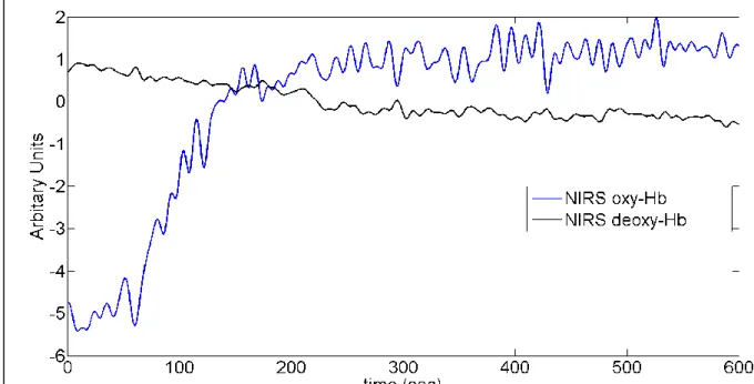
Figure 5. An illustrative example (subject 5) showing NIRS oxy-Hb (in blue) and NIRS deoxy-Hb (in black) signals. Small increase in deoxy-Hb signal and decrease in oxy-Hb signal was found at the beginning due to anodal HD-tDCS-evoked local neuronal activity increasing oxygen metabolism, that then caused vasodilation increasing regional cerebral blood flow and an increase in oxy-Hb signal, which then reduced deoxy-Hb signal, i.e., ‘metabolic hypothesis’ of neurovascular coupling.
Table 1
(Std. Dev. is standard deviation, CV is coefficient of variation )
pre HD-tDCS Parameters Subject 1 Subject 2 Subject 3 Subject 4 Subject 5 Mean±Std. Dev. (CV= Std. Dev/mean) 1 a 3.24 3.25 3.24 3.23 3.21 3.23±0.02 (±0.006) 2 a -3.73 -3.77 -3.76 -3.74 -3.72 -3.74±0.02 (±0.005) 3 a 1.78 1.77 1.79 1.72 1.71 1.75±0.04 (±0.023) 4 a -0.25 -0.26 -0.25 -0.24 -0.29 -0.26±0.02 (±0.077) 1 b 0.025 0.018 0.096 0.001 0.270 0.08±0.11 (±1.375) 2 b 0.016 0.001 0.061 0.664 0.001 0.15±0.29 (±1.933) 3 b 0.001 0.182 0.001 0.001 0.001 0.04±0.08 (±2.000) 4 b 0.001 0.147 0.001 0.001 0.001 0.03±0.07 (±2.333) 5 b 0.001 0.001 0.001 0.001 0.001 0.01±0.00 (±0.000) post HD-tDCS Parameters Subject 1 Subject 2 Subject 3 Subject 4 Subject 5 Mean±Std. Dev. (CV = Std. Dev/mean) 1 a 3.26 3.19 3.25 2.99 2.76 3.09±0.21 (±0.068) 2 a -3.79 -3.72 -3.74 -3.27 -2.98 -3.5±0.36 (±0.103) 3 a 1.79 1.84 1.73 1.59 1.62 1.71±0.10 (±0.059) 4 a -0.26 -0.32 -0.24 -0.31 -0.40 -0.31±0.06 (±0.194) 1 b -0.013 0.008 -0.014 -0.134 0.0752 -0.02±0.08 (±4.000) 2 b 0.029 -0.019 0.043 0.557 -0.006 0.12±0.25 (±2.083) 3 b -0.003 0.007 -0.029 -0.743 -0.225 -0.20±0.32 (±1.600) 4 b -0.028 0.009 -0.014 0.371 0.167 0.10±0.17 (±1.700) 5 b 0.015 -0.006 0.014 -0.051 -0.006 0.01±0.03 (±3.000) during HD-tDCS Parameter Subject 1 Subject 2 Subject 3 Subject 4 Subject 5 Mean±Std. Dev. (CV = Std. Dev/mean)