HAL Id: hal-01223573
https://hal.inria.fr/hal-01223573v2
Submitted on 15 Feb 2016
HAL is a multi-disciplinary open access
archive for the deposit and dissemination of
sci-entific research documents, whether they are
pub-lished or not. The documents may come from
teaching and research institutions in France or
abroad, or from public or private research centers.
L’archive ouverte pluridisciplinaire HAL, est
destinée au dépôt et à la diffusion de documents
scientifiques de niveau recherche, publiés ou non,
émanant des établissements d’enseignement et de
recherche français ou étrangers, des laboratoires
publics ou privés.
Are Static Schedules so Bad ? A Case Study on
Cholesky Factorization
Emmanuel Agullo, Olivier Beaumont, Lionel Eyraud-Dubois, Suraj Kumar
To cite this version:
Emmanuel Agullo, Olivier Beaumont, Lionel Eyraud-Dubois, Suraj Kumar. Are Static Schedules so
Bad ? A Case Study on Cholesky Factorization. IEEE International Parallel & Distributed Processing
Symposium (IPDPS 2016), May 2016, Chicago, IL, United States. �hal-01223573v2�
Are Static Schedules so Bad ?
A Case Study on Cholesky Factorization
Emmanuel Agullo, Olivier Beaumont, Lionel Eyraud-Dubois and Suraj Kumar Inria
LaBRI, University of Bordeaux – France
[email protected] , [email protected] , [email protected] , [email protected]
Abstract—Our goal is to provide an analysis and comparison of static and dynamic strategies for task graph scheduling on platforms consisting of heterogeneous and unrelated re-sources, such as GPUs and CPUs. Static scheduling strategies, that have been used for years, suffer several weaknesses. First, it is well known that underlying optimization prob-lems are NP-Complete, what limits the capability of finding optimal solutions to small cases. Second, parallelism inside processing nodes makes it difficult to precisely predict the performance of both communications and computations, due to shared resources and co-scheduling effects. Recently, to cope with this limitations, many dynamic task-graph based runtime schedulers (StarPU, StarSs, QUARK, PaRSEC) have been proposed. Dynamic schedulers base their allocation and scheduling decisions on the one side on dynamic information such as the set of available tasks, the location of data and the state of the resources and on the other hand on static information such as task priorities computed from the whole task graph. Our analysis is deep but we concentrate on a single kernel, namely Cholesky factorization of dense matrices on platforms consisting of GPUs and CPUs. This application encompasses many important characteristics in our context. Indeed, it involves 4 different kernels (POTRF, TRSM, SYRK and GEMM) whose acceleration ratios on GPUs are strongly different (from 2.3 for POTRF to 29 for GEMM) and it consists in a phase where the number of available tasks if large, where the careful use of resources is critical, and in a phase with few tasks available, where the choice of the task to be executed is crucial. In this paper, we analyze the performance of static and dynamic strategies and we propose a set of intermediate strategies, by adding more static (resp. dynamic) features into dynamic (resp. static) strategies. Our conclusions are somehow unexpected in the sense that we prove that static-based strategies are very efficient, even in a context where performance estimations are not very good.
Keywords- Runtime Systems, Scheduling, Accelerators, Cholesky, Heterogeneous Systems, Unrelated Machines.
I. INTRODUCTION
With the advent of multicore nodes and the use of ac-celerators, scheduling becomes notoriously difficult. Indeed, several phenomena are added to the inherent complexity of the underlying NP-hard optimization problem. First, the performance of the resources are strongly heterogeneous. For instance, in the case of the Cholesky factorization, some kernels are up to 29 times faster on GPUs with respect to CPUs whereas other kernels are only accelerated by a
factor of 2. In the literature, unrelated resources are known to make scheduling problems harder (see [1] for a survey on the complexity of scheduling problems and [2] for a recent survey in the case of CPU and GPU nodes). Second, internal node parallelism as well as shared caches and buses makes it difficult to precisely predict the execution time of a kernel on a resource, due to co-scheduling effects. These two observations led to the development of several dynamic schedulers, that make allocation and scheduling decisions at runtime, such as StarPU [3], StarSs [4], QUARK [5] or PaRSEC [6]. More specifically, these runtime schedulers see the application as a directed acyclic graph (DAG) of tasks where vertices represent tasks to be executed and edges dependencies between those tasks. Task priorities on this DAG are computed offline, for instance based on their estimated distance to the last task. Then, at runtime, the scheduler takes the scheduling and allocation decisions based on the set of ready tasks (tasks whose all data and control dependencies have been solved), on the availability of the resources (estimated using expecting processing and communication times), and on the priorities of the tasks. The HEFT heuristic [7] is certainly the most popular of this class of algorithms.
In this paper, our goal is to precisely assess the advantages and limitations of static (executed with possibly wrong estimations of execution times) and dynamic (computed online with basic greedy heuristics) strategies. We also design and evaluate a large set of intermediate solutions, by providing more static information to dynamic schedulers and by incorporating dynamic features into static schedules. Our study is rather deep than broad. In order to compare both approaches, we concentrate on a single dense linear algebra kernel, namely the Cholesky factorization (see description in Algorithm 1) on a single computing node consisting of CPUs and GPUs, and we compare and analyze the results under a variety of problem sizes for a large set of sophisticated schedulers. To simplify the comparison of the different approaches, throughout the text, we assume that it is possible to overlap communications with computations, and we do not explicitly take into account communication costs.
The outline of the paper is the following. Section II describes the tile Cholesky factorization algorithm and our
experimental framework. In Section III, we briefly describe works related to known static and dynamic schedulers for dense linear algebra kernels, together with known upper bounds for the Cholesky factorization. In Section IV, we discuss static strategies. In order to obtain the best possible schedule, we propose to use a constraint program (CP) whose use is limited to small and medium size problems due to its high cost. Then, we study the stability of optimal schedules under perturbations in kernel execution times. Using a large set of simulations, we prove that the optimal static schedule is in fact robust to realistic perturbations, and we furthermore add a dynamic work stealing strategy to better cope with those perturbations. In Section V, we study the behavior of the dynamic schedulers that can be found typically in runtime systems such as StarPU. We prove that these runtime systems make poor use of slow (CPU) resources, restricting their use to POTRF kernels for which they are best suited. This is due to very conservative allocation strategies, that we alleviate using sophisticated prediction schemes in order to improve their efficiency. In Section VI, we introduce a new class of dynamic schedulers, that are easy to implement. We prove that it is possible to improve their efficiency when injecting simple qualitative knowledge about the application. Then, we compare the best variants of all three approaches in Section VII and we prove that static schedule based strategies are better than dynamic ones, even in presence of bad performance estimates, what is an unexpected result and we finally propose conclusions and perspectives in Section VIII.
II. CONTEXT
A. Tile Cholesky Factorization
With the advent of multicore processors, so-called tile algorithms have been introduced to increase the level of parallelism and better exploit all the available cores [8]. Algorithm 1 for instance shows the pseudo-code of the tile
Algorithm 1: Tile Cholesky Factorization. for i= 0 . . . N − 1 do
A[i][i] ←POTRF(A[i][i]); for j= i + 1 . . . N − 1 do
A[j][i] ←TRSM(A[j][i], A[i][i]) ; for k= i + 1 . . . N − 1 do
A[k][k] ←SYRK(A[k][k], A[k][i]) ; for j= k + 1 . . . N − 1 do
A[j][k] ← GEMM(A[j][k], A[j][i], A[k][i]);
version of the Cholesky factorization, consisting of produc-ing a lower triangular matrix L from an input symmetric positive definite matrix A such that A = LL⊤. Matrix A
is decomposed into N × N square tiles. In each instance
of the outer loop, a Cholesky factorization (POTRFkernel) on the ith diagonal tile is performed and the trailing panel is updated with triangular solve (TRSM kernel). Then, the remaining trailing submatrix is updated by applying symmetric rank-k updates (SYRK kernel) on the diagonal tiles and general matrix multiplications (GEMM kernel) on non-diagonal tiles. Throughout all the paper, the color code for the different kernels presented in Algorithm 1 and in Figure 1 will be used.
This sequence of computation can be represented with a DAG (Directed Acyclic Graph) of tasks as depicted in Fig-ure 1 in the case of 5×5 tile matrix. Modern linear algebra
GEMM_4_2_1 TRSM_4_2 GEMM_4_2_0 GEMM_4_3_2 TRSM_4_3 GEMM_4_3_0 GEMM_4_3_1 SYRK_3_3_2 POTRF_3 SYRK_3_3_0 SYRK_3_3_1 SYRK_1_1_0 POTRF_1 GEMM_4_1_0 TRSM_4_1 TRSM_1_0 GEMM_2_1_0 GEMM_3_1_0 TRSM_2_1 SYRK_4_4_1 SYRK_4_4_2 SYRK_4_4_3 TRSM_4_0 SYRK_4_4_0 TRSM_3_1 POTRF_2 TRSM_3_2 POTRF_0 TRSM_3_0 TRSM_2_0 GEMM_3_2_1 GEMM_3_2_0 POTRF_4 SYRK_2_2_0 SYRK_2_2_1
Figure 1. DAG of the tile Cholesky factorization - 5×5 tile matrix.
libraries for multicore architectures (such as PLASMA [9] and FLAME [10]) implement these tile algorithms using a runtime system (QUARK [5] and SuperMatrix [11], respec-tively) for handling data dependencies and assigning tasks on available computational units using a dynamic scheduling policy. In the past few years, while GPUs have gained in popularity, tile algorithms have heavily been employed to handle heterogeneous architectures. In that case, the runtime system may assign part of the tasks to the GPUs to accelerate them. The MAGMA library has been extended following that trend [12] as well as the DPLASMA [13] library relying on the StarPU and PaRSEC runtime systems, respectively. Finally the CHAMELEON [14] platform has been designed in order to provide a framework for further studying those approaches with the ability to execute the same DAG transparently on multiple actual runtime systems (QUARK, StarPU or PaRSEC) or in simulation mode using advanced simulation tools such as SimGrid [15].
B. Experimental Framework
We consider a platform composed of nodes of two hexa-core Westmere Intel Xeon X5650 processors (12 CPU hexa-cores
kernel PORTF TRSM SYRK GEMM GPU/CPU ratio ≃2.3 ≃11 ≃26 ≃29
Table I
GPUACCELERATION RATIO OVERCPUCORE FOR ALL FOUR KERNELS.
per node) and three Nvidia Tesla M2070 GPUs (3 GPUs per node). As most runtime systems, StarPU dedicates one CPU core to efficiently exploit each GPU. As a consequence, we can view a node as being composed of 9 CPU workers and 3 GPU workers. We also observe that variance of different kernels on different resources are not so high and it is within the ±5 % of mean execution timings.
C. Comparing Static and Dynamic Schedulers
As stated in the introduction, our goal is to compare Static and Dynamic approaches when scheduling a DAG on a node consisting of both GPUs and CPUs. The Cholesky factorization is an excellent candidate to perform such a study. First, it is based (see Algorithm 1) on four different kernels that exhibit strongly heterogeneous performance and unrelated acceleration ratios on CPU cores and GPUs, as depicted in Table I. These timings have been obtained with the CHAMELEON [14] library running on top of the StarPU runtime system to assign tasks onto CPU cores or GPUs. CHAMELEON processes CPU tasks with the (sequential) Intel MKLlibrary and GPU tasks with the MAGMA(POTRF kernel) or CUBLAS (other kernels) libraries. Consistently
with [12], a tile size of 960 is being used.
Second, despite its regular nature, the Cholesky factor-ization induces complex dependencies and leaves a lot of freedom for scheduling. Indeed, the i-th POTRF releases N − i −1 TRSMs and these TRSMs release N − i − 1 inde-pendent SYRKs and (N −i−2)(N−i−1)2 independent GEMMs (see Algorithm 1). Moreover, dependencies between the different kernels are not trivial and there is no need to synchronize all kernels involving i, the outer loop index. For instance, the execution of most of the GEMMs induced by i-POTRF can be delayed and/or delegated to slow resources (GEMM_4_3_0 orSYRK_4_4_0 of Figure 1 can be delayed or delegated to slow resource).
Third, depending on the problem size, underlying schedul-ing problems are of very different natures. Throughout the text, all problem sizes will be expressed in terms of number of blocks, the tile size being maintained constantly equal to 960 as mentioned earlier. In the 8 × 8 case, it is crucial to perform tasks on the critical path as fast as possible, and it is not efficient to make use of all available resources. On the other hand, in the32 × 32 case, the scheduling problem is almost amenable (except at the very beginning and at the end) to an independent tasks problem, and the crucial issue is to make use of all available resources in a proportion that depends on the acceleration ratios given in Table I. Intermediate cases, such as the 12 × 12 case, are typically
hard, since both conflicting objectives (making an efficient use of resources and focus on the critical path) have to be simultaneously taken into account.
III. RELATED WORK
The problem of scheduling tasks with dependencies has been highly studied in the literature, starting from complex-ity and approximation analysis from Graham et al. [16]. Many dynamic algorithms have been proposed to solve this problem, in particular for the homogeneous case. In the specific setting of Cholesky factorization, reversing the task graph allows to identify provably optimal schedules for the homogeneous case, and the problem is now well understood [17], [18].
For the heterogeneous unrelated case, the literature is not as large. Most dynamic strategies are variants of the well-known heuristic HEFT [7] which combines a prior-itization of tasks by their distance to the exit node with a greedy strategy which places tasks so as to finish as early as possible. Other noteworthy approaches are based on work stealing [19], where idle resources steal available tasks from other resources, or on successively applying an algorithm for independent tasks scheduling on the set of ready tasks [2]. More static approaches have also been proposed to obtain more efficient schedules at the cost of longer running times. For instance, Constraint Programming is a paradigm which is widely used to solve many scheduling problems [20]. Branch-and-bound algorithms can also be designed for scheduling problems, with a wide range of search strategies [21], but the weakness of bounds in the heterogeneous case makes them less efficient than in the homogeneous case.
In this paper, we also use upper bounds on performance to assess the quality of the schedules obtained. Classical bounds in the homogeneous case are the area bound, defined as the total work divided by the number of processors, and the critical path, which is the maximum execution time over all paths in the graph. For the heterogeneous case, the area bound needs to be adapted, and can be defined as the solution of a linear program which expresses how many tasks of each type are scheduled on each resource. The critical path can also be expressed, however better results can be achieved when computing both bounds simultaneously, since this allows to express the tradeoff for critical tasks: if they are executed on faster resources but with poor acceleration, they improve the critical path but degrade the area bound. Such a mixed bound has been proposed [22], and in this paper we use an improved version (named iterative bound) which iteratively adds new critical paths until all are taken into account.
IV. STATIC STRATEGIES
In this Section, we describe schedules obtained with a previously proposed Constraint Programming formulation
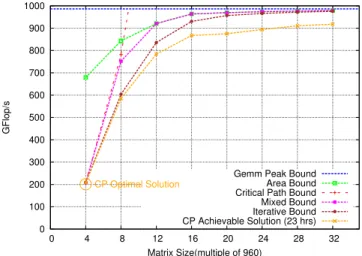
for the scheduling problem [22], and we analyze their robustness to errors in computation times. The computing time needed to obtain a good schedule depends on the size of the task graph (number of tasks and dependences) and of the platform description (number of choices for each task). In our case, the number of choices is limited to deciding whether a task is allocated to CPU or GPU; however the number of tasks grows as a cubic function of the matrix size. For this reason, it is possible to obtain nearly optimal solution for small matrices and good solution for intermedi-ate matrices in a few hours. But the solutions obtained for large matrices are far from optimal, and most of the dynamic strategies achieve better timings than those solutions (see dynamic strategies). Figure 2 provides a comparison of the solution obtained from this formulation with the bounds discussed in the previous section. This graph shows how the iterative bound is able to improve over previous bounds, and how the CP formulation is able to compute almost optimal solutions for small cases.
0 100 200 300 400 500 600 700 800 900 1000 0 4 8 12 16 20 24 28 32 GFlop/s Matrix Size(multiple of 960) CP Optimal Solution
Gemm Peak Bound Area Bound Critical Path Bound Mixed Bound Iterative Bound CP Achievable Solution (23 hrs)
Figure 2. Upper bounds and CP feasible solution performance.
In order to determine the stability of CP schedules, we use 30 different sets of execution timings by introducing some randomness (in the range of -10 to 10%) in the original execution timings of tasks on each resource. We normalized execution timings with respect to the area bound of the corresponding task graph, so that the area bound of all sets of execution timings for a given matrix size corresponds to the same value. For each of these generated execution timings, we use the same static schedule (obtained with CP formulation using the original timings) by keeping on each resource the same allotted tasks in the same order (of course start times may be different because of the changes in execution times). Figure 3 shows the performance ratio of each of the obtained schedules compare to the iterative bound for the 12×12 tile matrix, in which experiment number 0 corresponds to the original execution timings. On other experiments, the performance degradation is below 10
0.86 0.88 0.9 0.92 0.94 0.96 0.98 1 1.02 1.04 0 5 10 15 20 25 30
Performance Ratio WRT Iterative Bound
Experiment Number
SS reference (IterativeBound)
Figure 3. Performance ratio of static schedules with respect to iterative
bound- 12 × 12 tile matrix.
% compared to performance ratio of the static schedule on the original timings. Using this static schedule can therefore be a reasonable option for intermediate size matrices – but obtaining a good solution is the hard part. In all the rest of the paper, the static strategy will be denoted as SS. A. Some dynamic strategies with static schedule
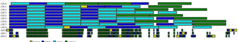
Though performance degradation is limited in presence of perturbations, we observed in the obtained schedules that some GPU resource remain significantly idle in some experiments. Figure 4(a) shows the trace of one of the experiments with perturbed execution timings. Here one of our critical resource (GPU1) is idle for a significant amount of time in the middle of execution, because the next task that should be executed on this resource is not ready yet (remember that we keep the order as given by the CP solution). This observation is a motivation to improving the performance by injecting dynamic corrections to the static schedules.
The acceleration factor of GEMM tasks is highest on GPU among all Cholesky tasks. Therefore we allowed an ideal GPU worker to help other workers by executing the GEMM tasks of other workers. When a GPU worker is Idle and waiting for some task to become ready, then it searches for highest priority ready GEMM in its own list and then in the list of other workers, and executes it if one is found. We name SS+G such a correction to the original SS. This strategy improves the performance of SS slightly but does not eliminate all idle time from GPUs in the middle of execution. Therefore we also consider stealing SYRK tasks, whose acceleration factor on GPU is second highest (after GEMM acceleration factor). We name SS+GS such a correction to the original SS. Figure 4 shows the comparison of trace with SS (Figure 4(a)) and SS+GS (Figure 4(b)).
3 0 0 3 3 3 8 3 1 11 9 5 11 11 7 0 0 9 6 2 8 8 8 5 5 10 10 9 9 0 5 1 7 2 0 11 6 7 8 11 0 2 4 2 0 11 11 9 3 4 11 11 0 5 5 9 1 1 9 9 5 10 5 10 6 0 6 6 0 9 9 9 2 7 4 6 11 5 0 6 5 10 2 0 7 7 0 11 10 1 10 1 6 2 11 3 2 9 9 3 9 9 0 10 10 8 2 4 6 4 4 10 8 0 1 0 0 1 1 2 0 0 4 10 6 10 5 40 6 40 2 2 2 1 0 10 40 10 21 8 41 2 2 0 10 50 10 60 3 13 1 11 1 1 3 20 7 40 4 30 8 31 10 40 9 40 11 51 8 30 9 21 4 31 10 21 6 61 6 55 2 1 9 31 9 41 7 62 8 32 4 32 6 6 5 3 2 6 51 7 56 3 2 8 51 9 52 7 32 7 62 10 32 10 44 5 5 3 6 52 8 73 10 52 7 54 10 58 4 11 4 3 11 54 11 53 6 6 2 9 64 6 56 5 5 6 6 4 7 60 11 84 8 73 9 53 9 43 9 77 6 4 9 64 9 73 9 85 9 75 8 65 9 80 10 93 11 78 7 2 11 83 11 84 11 83 10 94 10 95 11 85 10 99 8 10 7 1 11 102 11 103 11 107 10 811 7 7 11 85 11 1010 9 9 10 1010 11 10 11 5 0 10 0 8 0 0 8 10 8 40 4 4 0 8 66 1 0 8 8 0 8 21 6 40 5 11 4 4 1 6 20 10 80 11 10 7 10 3 20 7 30 10 30 6 311 2 1 7 30 7 20 9 31 10 60 11 41 10 30 5 31 5 31 5 41 10 51 9 20 8 70 7 52 5 31 10 100 9 7 4 3 3 4 4 2 6 33 5 5 0 11 72 11 51 9 62 7 42 10 85 4 2 10 53 7 62 9 510 4 3 11 41 10 73 8 53 8 62 10 62 11 111 9 71 9 82 9 44 6 6 1 7 7 4 8 64 7 53 7 7 2 10 103 8 8 4 8 8 4 7 7 3 9 64 10 65 7 7 5 10 6 6 7 7 4 10 71 11 75 10 75 8 75 8 8 9 6 6 8 76 8 8 1 10 92 10 96 9 82 11 93 11 63 11 95 11 64 9 9 5 11 75 9 9 6 9 9 7 9 9 4 11 96 10 86 10 96 10 106 11 810 8 8 10 911 8 8 11 911 9 6 11 117 11 11 10 11 11 6 0 4 0 0 10 10 2 10 8 50 5 20 4 24 1 8 1 0 6 21 8 61 4 21 8 21 8 8 0 9 10 11 20 11 37 1 1 11 23 2 1 11 31 7 41 6 30 11 91 7 21 10 82 11 30 10 71 5 21 3 3 2 3 3 0 7 61 5 5 2 5 5 1 11 52 4 4 2 5 42 8 42 6 40 9 53 5 41 8 51 11 43 6 41 8 72 11 47 3 3 7 410 3 3 10 42 9 30 9 83 8 42 8 63 10 83 8 71 11 112 10 74 8 53 10 62 9 73 10 73 7 52 7 7 3 11 117 5 3 10 105 7 64 10 102 9 89 4 4 9 59 5 5 9 62 11 74 9 88 6 1 11 61 11 86 9 77 8 8 2 11 69 7 7 9 84 11 64 11 76 10 711 6 6 11 75 10 88 9 9 5 11 96 11 94 11 107 10 97 10 107 11 98 10 10 6 11 107 11 108 11 109 11 108 11 119 11 11
POTRF TRSM SYRK GEMM
CPU0 CPU1 CPU2 CPU3 CPU4 CPU5 CPU6 CPU7 CPU8 GPU0 GPU1 GPU2
(a) Static trace.
3 0 0 3 3 3 8 3 1 11 9 5 11 11 7 0 0 9 6 2 8 8 8 5 5 10 10 9 9 0 5 1 7 2 0 11 6 7 8 11 0 2 4 2 0 11 11 9 3 4 11 11 0 5 5 9 1 1 9 9 5 10 5 10 6 0 6 6 0 9 9 9 2 7 4 6 11 5 0 6 5 10 2 0 7 7 0 11 10 1 10 1 6 2 11 3 2 9 9 3 9 9 0 10 10 8 2 4 6 4 4 10 8 0 1 0 0 1 1 2 0 0 4 10 6 10 5 40 6 40 2 2 2 1 0 10 40 10 21 8 41 2 2 0 10 50 10 60 3 13 1 11 1 1 3 20 7 40 4 30 8 31 10 40 9 40 11 51 8 30 9 21 4 31 10 21 6 6 1 9 31 6 55 2 1 9 41 7 62 8 32 4 32 6 6 5 3 2 6 51 7 56 3 2 8 51 9 52 7 32 7 62 10 32 10 44 5 5 3 6 52 8 73 10 52 7 54 10 58 4 11 4 3 11 54 11 53 6 6 2 9 64 6 56 5 5 6 6 4 7 60 11 84 8 73 9 53 9 80 10 97 6 4 9 64 9 75 9 75 8 65 9 83 11 72 11 88 7 3 10 94 11 84 10 95 11 85 10 95 11 96 11 99 8 10 7 7 10 911 7 7 11 86 11 107 11 1010 9 9 10 1010 11 10 10 11 1111 5 0 10 0 8 0 0 8 10 8 40 4 4 0 8 60 8 26 1 0 8 8 1 6 41 4 4 0 10 81 6 21 8 20 11 10 7 10 3 20 7 30 10 30 6 31 7 311 2 0 7 20 9 31 10 60 11 41 10 30 5 31 5 31 5 41 10 51 9 20 8 70 7 50 9 70 11 72 5 31 10 102 6 32 11 51 10 74 3 3 4 4 3 5 5 2 7 41 9 71 9 62 10 82 10 52 9 55 4 2 10 63 7 61 9 83 11 43 8 510 4 3 8 62 9 41 11 72 11 114 8 52 9 73 7 54 8 64 6 6 1 7 7 3 9 64 7 53 7 7 2 10 103 8 8 4 8 8 4 7 7 5 7 7 1 11 83 9 45 10 65 10 71 10 95 8 76 7 7 5 8 8 2 10 99 6 6 9 73 11 64 11 66 8 8 6 9 83 11 83 11 94 11 94 9 9 5 11 65 11 75 9 9 6 9 9 7 9 9 6 11 86 10 10 8 9 9 2 11 103 11 104 11 1010 8 8 10 911 8 8 11 911 9 9 11 108 11 119 11 11 6 0 4 0 0 5 10 10 10 2 10 8 50 5 20 4 24 1 8 1 0 6 21 8 61 4 21 8 8 0 9 10 11 20 11 37 1 1 11 21 11 33 2 1 7 41 6 30 11 91 7 21 10 82 11 30 10 71 5 21 3 3 2 3 3 0 7 61 5 5 1 11 52 5 5 2 4 4 2 5 42 8 42 6 40 9 51 8 53 5 41 11 41 8 72 11 43 6 42 9 30 9 87 3 3 7 410 3 3 10 43 8 42 8 63 10 83 8 71 11 112 10 73 10 63 10 72 9 82 11 74 10 62 7 7 3 11 114 10 77 5 3 10 105 7 64 10 103 9 79 4 4 9 59 5 4 9 85 9 61 11 62 11 68 6 6 8 74 11 72 11 97 8 8 9 7 7 9 86 10 711 6 6 11 76 10 91 11 105 10 86 10 87 10 87 10 105 11 107 11 98 10 108 11 106 11 117 11 11
POTRF TRSM SYRK GEMM
CPU0 CPU1 CPU2 CPU3 CPU4 CPU5 CPU6 CPU7 CPU8 GPU0 GPU1 GPU2 (b) SS+GS trace.
Figure 4. Trace with perturbed timings for 12 × 12.
0.86 0.88 0.9 0.92 0.94 0.96 0.98 1 1.02 1.04 0 5 10 15 20 25 30
Performance Ratio WRT CP Schedule
Experiment Number
SS+GS reference (SS)
Figure 5. Performance improvement of SS+GS over original SS obtained with CP - 12 × 12 tile matrix.
with SS improves the scheduler performance in most of the experiments. while its adverse effect on a few experiments is very negligible (performance degradation is less than 1 %). This allows to obtain good and stable solutions when compared to the iterative bound, even in presence of noisy execution timings.
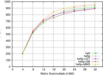
V. HEFT-LIKE SOLUTIONS(DYNAMIC,TASK-CENTRIC) We use heft (heterogeneous early finish time) and heftp (heterogeneous early finish time with priority) schedulers, which are based on a very well know state-of-the-art task centric HEFT heuristic. When a tasks is ready, both algo-rithms put it in the queue of the resource that is expected to complete it first, given the expected available time of the resource and the expected running time of the task on this resource. The only difference between heft and heftp is the use of priorities. In heftp, task priorities are computed offline
based on the longest path from the task to last task in the DAG, using minimum expected execution timing of each task in presence of heterogeneous resources, as proposed in [7]. Then, heftp schedules ready tasks ordered by their priorities to workers queues and in turn, each worker selects and schedules the task from its own queue with the highest priority. 0 100 200 300 400 500 600 700 800 900 1000 0 4 8 12 16 20 24 28 32 GFlop/s Matrix Size(multiple of 960) heft heftp heftp+LET heftp+GB heftp+MMS
Figure 6. Performance with different heft schedulers
In Figure 6, we can observe that heftp outperforms heft for all matrix sizes, thanks to its capability on executing in priority tasks on or close to the critical path.
1 2 3 4 5 6 7 8
0 1 0 4 0 0 2 2 0 4 20 3 3 0 5 17 0 0 5 42 1 1 2 2 1 3 25 1 0 6 31 5 40 7 20 8 15 2 1 7 22 4 32 6 31 6 42 6 410 0 1 5 5 6 3 1 7 43 4 4 2 7 33 5 5 0 9 20 7 57 3 0 8 45 4 4 5 5 3 6 52 8 30 6 6 1 8 44 6 57 4 1 10 20 10 32 9 311 1 4 6 6 0 9 54 7 59 3 1 8 62 9 40 8 73 8 50 11 34 7 61 7 7 11 2 1 9 62 10 42 8 73 9 50 10 62 9 63 10 41 9 73 8 74 9 50 9 85 7 7 10 4 4 8 70 11 62 10 64 9 63 9 75 8 72 9 85 9 63 8 8 4 9 71 10 80 10 93 10 78 7 5 8 8 4 11 54 9 86 8 8 1 11 81 9 9 4 11 60 11 92 10 93 11 72 9 9 5 11 61 11 93 9 9 3 11 84 10 95 11 71 11 104 11 86 9 9 6 11 77 9 9 5 11 811 7 9 7 11 86 11 95 11 106 10 102 11 118 11 94 11 119 10 105 11 116 11 117 11 118 11 119 11 1111 2 0 5 0 0 3 10 4 10 5 30 6 10 4 4 0 7 14 1 1 4 4 1 3 3 8 0 7 1 1 5 31 6 30 6 44 2 2 3 3 2 5 30 8 27 2 0 9 10 7 49 1 4 3 3 5 42 5 5 0 10 12 6 51 8 32 7 41 7 511 0 0 9 39 2 0 8 52 7 51 9 38 3 2 6 6 3 7 56 5 3 8 40 11 210 2 5 6 6 0 10 48 4 1 9 50 7 7 2 10 30 9 61 10 41 8 72 9 54 8 51 11 35 7 63 7 7 1 10 52 11 37 6 0 11 52 10 511 3 2 11 40 10 72 9 76 7 7 0 8 8 1 11 58 6 1 8 8 3 11 42 11 52 10 76 8 710 5 3 9 84 8 8 9 6 0 11 82 10 83 11 61 10 90 9 9 11 5 3 10 85 9 87 8 8 5 10 79 7 3 10 94 11 77 9 84 9 9 10 7 9 8 0 10 105 10 92 11 106 10 98 9 9 3 11 1010 8 3 10 105 11 98 10 90 11 1110 9 1 11 116 11 103 11 118 10 108 11 1010 11 10 10 11 11 3 0 0 1 1 0 2 10 3 26 0 0 4 30 5 20 6 23 1 1 4 21 4 36 1 1 5 21 6 29 0 3 2 6 2 2 4 4 2 5 40 7 38 1 0 5 5 0 6 55 3 1 7 31 8 21 6 50 8 33 6 48 2 1 9 26 4 0 7 610 1 3 7 40 10 21 6 6 1 7 60 11 10 9 42 8 41 8 53 6 6 0 8 62 7 61 9 42 8 51 10 33 7 61 11 27 5 2 8 63 9 40 10 510 3 2 7 7 3 8 60 11 49 4 0 9 78 5 4 8 64 7 7 1 11 41 10 63 9 65 8 63 10 59 5 1 9 81 10 74 10 50 10 82 8 8 1 11 63 10 611 4 0 11 73 11 52 11 64 10 61 11 75 9 75 10 62 11 74 10 76 9 710 6 2 11 84 10 86 9 86 10 70 11 105 10 811 6 2 11 95 9 9 6 10 83 11 91 10 107 10 84 11 92 10 106 11 87 10 94 10 104 11 105 10 1011 8 7 11 97 10 107 11 1011 9 9 11 10
POTRF TRSM SYRK GEMM
CPU0 CPU1 CPU2 CPU3 CPU4 CPU5 CPU6 CPU7 CPU8 GPU0 GPU1 GPU2
Figure 7. heftptrace for 12 × 12
Although heftp outperforms heft, we can observe on Figure 7 that the allocation dynamically computed by heftp is far from optimal since it wastes most of CPU resources. Indeed, only CPU 0 is used to process tasks, and its use is restricted to the execution of POTRFs, that are the most efficient kernel on CPUs (see Table I). Therefore, in practice, heftp is too conservative and the running times on CPUs and GPUs are so different that for all tasks (excepts a few POTRFs), the expected completion time is always smaller on one of the GPUs. On the other hand, we have observed that there are tasks (typically GEMMs and SYRKS) that are released early in the execution but whose results are needed late. Such tasks are typically good candidates to be executed on CPUs. In practice, they are released early and at the time when they are allocated by heftp on a GPU, their expected completion time is small. On the other hand,
since their priority is low, they will be consistently passed over by other tasks once in the GPU queue, so that their actual completion time on the GPU is in fact larger than their expected completion on a CPU.
A. Improvement of heftp Scheduler
Following this observation and in order to improve heftp performance by making good use of all CPU resources , we modify heftp scheduler such that scheduling decision is not only based on the minimum completion time heuristic but also based on certain look-ahead information.
1) heftp+LET (Local Execution time): In this strategy, before making a scheduling decision for a ready task t, the scheduler first computes the minimum expected completion time on a CPU (ecpu) and then simulates the execution
of heftp until task t completes execution (ehef tp) on some
(GPU) worker. If ecpu ≤ehef tp, that typically corresponds
to the situation described above where t has been passed over by many higher priority tasks in the GPU queue, then heftp+LET schedules task t on a CPU.
2) heftp+GB (GPU Busy): In this strategy, heftp+GB always tries to assign task t on a CPU and then simulates the execution of heftp until the completion time of task t on a CPU (ecpu). Then, it checks whether all GPUs have been
busy between the current time and ecpu. If it is the case,
then heftp+GB assumes that it is safe to schedule t on a CPU; otherwise, t is scheduled on a GPU.
3) heftp+MMS (Min Makespan): In this (higher cost) strategy, scheduler selects for task t a CPU worker if and only if it improves the overall makespan. To determine whether it is the case, heftp+MMS simulates the execution of heftp until the end, with t forced on a CPU and t allocated according to heftp. If the simulation time is smaller with t forced on a CPU, then heftp+MMS allocates t on this CPU. B. Analysis of different Improvedheftp Scheduler
Figure 6 describes the performance of the different heftp heuristics. heftp+LET and heftp+GB strategies use simula-tion upto certain lookahead (until task completes execusimula-tion in heftp+LET and until task completes execution on CPU in heftp+GB). Therefore, this adds an acceptable overhead to the scheduler and it results in a larger use of CPU resources. This induces a positive effect on the overall makespan for small to medium size cases, as shown in Figure 6.
But making the good utilisation of CPUs does not guar-antee to improve the performance! Indeed, heftp+LET and heftp+GBstrategies schedule significant amount of GEMMs and SYRKs on CPUs, i.e. tasks that are not well suited to CPUs (see Table I). On the other hand, when the size of the problem becomes large, the problem is of different nature, since all heuristics keep all resources (CPU and GPU) busy most of the time. Then, the critical path bound becomes less important than the area bound and what becomes crucial is to allocate tasks on the best suited resources, what is
better achieved by heftp. heftp+MMS strategy is based on the estimation of the overall completion time, and therefore does not suffer from these limitations for large sizes (see Figure 6). On the other hand, it induces a (too) large scheduling overhead to be used in practice, due to the simulation cost.
VI. HETEROPRIO-LIKE SOLUTIONS(DYNAMIC,
RESOURCE-CENTRIC) A. Baseline HeteroPrio scheduler
HEFT-like heuristics are task-centric as they first select a particular task before attributing it to a particular resource. One drawback of this class of greedy heuristics is that they may attribute a considered task (say a POTRF) to a given resource (say a GPU) because at decision time it is the best suited with respect to the expected completion time, conducting not to schedule another available task (say a GEMM) to be executed on that resource whereas it would have better fit it with respect to the acceleration factor. One option to overcome this limit consists of injecting static knowledge to the heuristic as discussed above. A most drastic alternative consists of designing another class, resource-centric of heuristics that aim at selecting the task that achieves the best acceleration factor for a given re-source. Such an approach is relatively natural in the case of independent tasks and was first introduced in [23] under the name of HeteroPrio (HP) to enhance task-based fast multipole methods (FMM) whose computation is dominated by independent tasks. We investigate such an alternative approach that we implement with the following design. Multiple scheduling queues are instantiated, each queue aiming at collecting tasks of acceleration factors of same magnitude. In the baseline version that we propose we consider one queue per type of task (hence four in total). Whenever a worker is idle it polls for a task within the set of ready queues and selects the one which best suits to this worker. In our case, CPU cores hence poll POTRF, TRSM, SYRK and GEMM queues whereas GPU poll the queues in reverse order. To favor progress, within a queue, GPU (resp. CPU) choose the highest (resp. lowest) priority task.
0 2 2 6 1 1 6 6 1 11 10 2 11 10 9 5 6 9 7 4 0 0 4 4 11 1 1 11 11 3 6 3 9 3 3 9 9 5 11 9 5 0 0 5 5 10 1 1 10 10 10 2 2 10 10 4 11 11 4 10 9 6 11 8 6 0 0 6 6 9 1 1 9 9 9 2 2 9 9 4 6 6 5 6 6 6 7 7 7 0 0 7 7 8 1 1 8 8 8 2 2 8 8 4 11 7 5 11 7 8 0 0 8 8 7 1 1 7 7 7 2 2 7 7 3 7 7 4 7 7 10 6 6 11 10 9 0 0 9 9 5 1 1 5 5 2 5 5 10 3 3 10 10 4 11 10 6 10 10 7 10 9 10 0 0 10 10 4 1 1 4 4 2 4 4 3 5 5 10 4 4 10 10 11 6 6 11 11 7 11 9 11 0 0 11 11 1 2 2 2 11 2 2 11 11 8 3 11 5 4 9 9 5 9 9 7 9 9 0 3 0 0 3 3 0 3 1 0 4 30 5 10 5 30 5 40 8 10 8 20 7 40 7 50 9 30 8 50 10 30 9 50 11 30 11 40 11 50 11 60 10 90 11 10 1 11 61 4 21 5 31 6 41 6 51 9 21 9 31 8 51 8 61 8 71 11 41 11 51 10 81 11 84 2 2 4 32 5 42 6 5 2 11 52 11 611 3 3 11 5 2 10 52 7 32 7 52 7 62 8 62 9 63 6 42 10 72 11 72 11 94 5 4 11 4 4 7 63 10 43 10 73 9 53 9 73 8 43 8 73 11 87 5 5 7 64 8 74 9 83 11 105 8 8 4 10 54 10 85 10 85 11 11 5 9 8 5 10 109 6 6 8 8 6 10 9 6 11 9 7 11 11 10 9 9 10 1010 11 10 11 2 0 0 3 20 1 13 1 1 3 3 0 4 20 5 20 6 20 6 30 6 40 6 50 8 30 10 10 7 60 11 10 8 60 10 40 9 60 9 70 9 80 10 80 11 81 6 3 1 11 31 4 31 5 41 7 31 7 41 7 51 7 61 9 41 9 51 9 61 9 71 9 81 11 71 11 95 2 2 5 32 6 42 6 6 2 11 44 3 3 11 4 2 10 42 7 42 8 42 8 52 9 52 9 73 6 52 10 82 10 93 4 4 3 11 113 7 53 7 66 4 4 6 54 11 53 10 54 5 53 9 43 10 93 8 53 9 83 8 8 8 4 4 8 54 9 54 9 74 11 98 5 5 8 74 10 610 5 5 10 75 11 8 5 9 7 5 7 78 6 6 9 8 5 11 10 6 10 86 9 910 7 7 8 8 8 10 8 7 10 108 10 10 7 11 108 11 11 8 11 911 9 9 11 10 10 11 11 1 0 0 2 11 2 1 1 3 2 0 4 10 6 10 7 10 7 20 7 30 9 10 9 20 8 40 10 20 9 40 11 20 8 70 10 50 10 60 10 70 11 70 11 91 6 2 1 11 21 5 21 7 21 8 21 8 31 8 41 10 21 10 31 10 41 10 51 10 61 10 71 10 93 2 2 3 3 6 2 2 6 3 2 11 35 3 3 5 4 2 10 32 8 32 9 32 9 42 8 72 10 62 9 83 11 62 11 83 6 6 7 3 3 7 43 11 77 4 4 7 54 11 63 10 65 3 9 63 11 93 8 63 10 86 5 9 4 4 8 64 9 64 11 84 8 85 8 64 10 75 10 65 11 6 5 9 6 6 7 6 6 8 7 5 10 9 6 10 77 8 7 7 10 86 11 711 7 9 7 7 9 89 8 7 11 811 8 8 11 108 9 9 9 8 10 99 11 11
POTRF TRSM SYRK GEMM CPU0 CPU1 CPU2 CPU3 CPU4 CPU5 CPU6 CPU7 CPU8 GPU0 GPU1 GPU2
Figure 8. 12 × 12 trace with heteroprio scheduler.
Figure 8 presents a 12 × 12 HP execution trace. Because nothing prevents CPU to process a task when idle in the baseline version of HP, CPU get attributed tasks that induce GPU starvation while being executed, which may potentially lead to significant performance degradations. Furthermore, in this baseline version, progress is only ensured with the
ordering of tasks within a queue. This strategy which aggres-sively favors the acceleration of tasks may be insufficient to ensure a global progress along the critical path, eventually leading to starvation. This is why GPUs are periodically starving in the trace.
B. Improved HeteroPrio algorithms
We now propose successive corrections to the baseline version of HP in order to find a better trade-off between acceleration of tasks and progress.
1) HP+Sp: The first correction we introduce consists of preventing immediate GPU starvation thanks to the follow-ing spoliation (Sp) rule. When a GPU is starvfollow-ing while at least one CPU is being executing a task, the execution of the highest priority task being executed on CPU is aborted and attributed to the GPU.
2) HP+CGV: Defining multiple queues for tasks whose acceleration factors are of roughly the same magnitude may provide only a limited advantage in terms of acceleration but a severe penalty in terms of progress. For this reason, in addition to HP+Sp correction, we propose that GPUs get a combined view (CGV) of GEMM, SYRK and TRSM ready queues whose acceleration factor is in a relatively thin range of values ([11; 29]) with respect to the distance to POTRF acceleration factor (2.3).
3) HP+PP: Because POTRF has a very low acceleration factor with respect to other kernels, we propose to favor its execution on CPU with the following preemption rule in addition to HP+CGV correction. If all workers are busy when a POTRF becomes ready, the lowest priority task being executed on CPU is aborted and set back to the ready queue so that the considered POTRF task can be immediately attributed to that CPU. In this case, preemption is only applied to POTRF, so we call it POTRF preemption (PP).
4) HP+PC: When a CPU is selecting a task, that task may have a relatively low priority with respect to other ready tasks in that queue. However other tasks with lower priority may become ready while that task is being processed. If a GPU becomes free at that time, it may thus have to pick up one of those new low priority ready tasks and potentially prevent fast progress on the critical path. To overcome this issue due to the greedy nature of HP, we propose to forbid a GPU to pick up a ready task with a lower priority than a task being executed on CPU. For that, we introduce the following additional spoliation rule. If no ready task has priority higher than all tasks being executed on CPU, then GPU spoliates the highest priority task being executed on CPU. This additional spoliation enhances on GPU thanks to a Priority Constraint (PC). This strategy is quite restrictive and allows only few tasks to run on CPU.
5) HP+PCEP: We therefore propose a variant where the previous PC spoliation rule does not apply to POTRF, which we name Priority Constraint Except POTRF (PCEP).
6) HP+PCEPT: If PC spoliation is excepted for both POTRF and TRSM, the rule is then called Priority Constraint Except POTRF and TRSM (PCEPT).
000000 000000 000000 000000 000000 000000 000000 000000 000000 000000 111111 111111 111111 111111 111111 111111 111111 111111 111111 111111 00 00 00 00 00 00 00 00 00 00 11 11 11 11 11 11 11 11 11 11 000 000 000 000 000 000 000 000 000 000 111 111 111 111 111 111 111 111 111 111 000000000 000000000 000000000 000000000 000000000 000000000 000000000 000000000 000000000 000000000 111111111 111111111 111111111 111111111 111111111 111111111 111111111 111111111 111111111 111111111 000000000 000000000 000000000 000000000 000000000 000000000 000000000 000000000 000000000 111111111 111111111 111111111 111111111 111111111 111111111 111111111 111111111 111111111 0000000000 1111111111 00000000000000 00000000000000 00000000000000 00000000000000 00000000000000 00000000000000 00000000000000 00000000000000 00000000000000 00000000000000 11111111111111 11111111111111 11111111111111 11111111111111 11111111111111 11111111111111 11111111111111 11111111111111 11111111111111 11111111111111 000000000 000000000 000000000 000000000 000000000 000000000 000000000 000000000 000000000 111111111 111111111 111111111 111111111 111111111 111111111 111111111 111111111 111111111 00000000000000 00000000000000 00000000000000 00000000000000 00000000000000 00000000000000 00000000000000 00000000000000 00000000000000 00000000000000 11111111111111 11111111111111 11111111111111 11111111111111 11111111111111 11111111111111 11111111111111 11111111111111 11111111111111 11111111111111 0000000000000000000000000000 0000000000000000000000000000 0000000000000000000000000000 0000000000000000000000000000 0000000000000000000000000000 0000000000000000000000000000 0000000000000000000000000000 0000000000000000000000000000 0000000000000000000000000000 0000000000000000000000000000 1111111111111111111111111111 1111111111111111111111111111 1111111111111111111111111111 1111111111111111111111111111 1111111111111111111111111111 1111111111111111111111111111 1111111111111111111111111111 1111111111111111111111111111 1111111111111111111111111111 1111111111111111111111111111 00000000000000000000000000000 00000000000000000000000000000 00000000000000000000000000000 00000000000000000000000000000 00000000000000000000000000000 00000000000000000000000000000 00000000000000000000000000000 00000000000000000000000000000 00000000000000000000000000000 11111111111111111111111111111 11111111111111111111111111111 11111111111111111111111111111 11111111111111111111111111111 11111111111111111111111111111 11111111111111111111111111111 11111111111111111111111111111 11111111111111111111111111111 11111111111111111111111111111 0000 0000 0000 0000 0000 0000 0000 0000 0000 0000 1111 1111 1111 1111 1111 1111 1111 1111 1111 1111 000000000 111111111 00000000000000 00000000000000 00000000000000 00000000000000 00000000000000 00000000000000 00000000000000 00000000000000 00000000000000 00000000000000 11111111111111 11111111111111 11111111111111 11111111111111 11111111111111 11111111111111 11111111111111 11111111111111 11111111111111 11111111111111 000000000000000000000000000000000000 000000000000000000000000000000000000 000000000000000000000000000000000000 000000000000000000000000000000000000 000000000000000000000000000000000000 000000000000000000000000000000000000 000000000000000000000000000000000000 000000000000000000000000000000000000 000000000000000000000000000000000000 000000000000000000000000000000000000 111111111111111111111111111111111111 111111111111111111111111111111111111 111111111111111111111111111111111111 111111111111111111111111111111111111 111111111111111111111111111111111111 111111111111111111111111111111111111 111111111111111111111111111111111111 111111111111111111111111111111111111 111111111111111111111111111111111111 111111111111111111111111111111111111 00000000000000000000 00000000000000000000 00000000000000000000 00000000000000000000 00000000000000000000 00000000000000000000 00000000000000000000 00000000000000000000 00000000000000000000 11111111111111111111 11111111111111111111 11111111111111111111 11111111111111111111 11111111111111111111 11111111111111111111 11111111111111111111 11111111111111111111 11111111111111111111 00000000000000 00000000000000 00000000000000 00000000000000 00000000000000 00000000000000 00000000000000 00000000000000 00000000000000 00000000000000 11111111111111 11111111111111 11111111111111 11111111111111 11111111111111 11111111111111 11111111111111 11111111111111 11111111111111 11111111111111 0000000000000000000000000000000000 0000000000000000000000000000000000 0000000000000000000000000000000000 0000000000000000000000000000000000 0000000000000000000000000000000000 0000000000000000000000000000000000 0000000000000000000000000000000000 0000000000000000000000000000000000 0000000000000000000000000000000000 0000000000000000000000000000000000 1111111111111111111111111111111111 1111111111111111111111111111111111 1111111111111111111111111111111111 1111111111111111111111111111111111 1111111111111111111111111111111111 1111111111111111111111111111111111 1111111111111111111111111111111111 1111111111111111111111111111111111 1111111111111111111111111111111111 1111111111111111111111111111111111 0000000000000000 0000000000000000 0000000000000000 0000000000000000 0000000000000000 0000000000000000 0000000000000000 0000000000000000 0000000000000000 0000000000000000 1111111111111111 1111111111111111 1111111111111111 1111111111111111 1111111111111111 1111111111111111 1111111111111111 1111111111111111 1111111111111111 1111111111111111 00000000000 00000000000 00000000000 00000000000 00000000000 00000000000 00000000000 00000000000 00000000000 00000000000 11111111111 11111111111 11111111111 11111111111 11111111111 11111111111 11111111111 11111111111 11111111111 11111111111 0000 0000 0000 0000 0000 0000 0000 0000 0000 0000 1111 1111 1111 1111 1111 1111 1111 1111 1111 1111 0000000000000000000000000000000 0000000000000000000000000000000 0000000000000000000000000000000 0000000000000000000000000000000 0000000000000000000000000000000 0000000000000000000000000000000 0000000000000000000000000000000 0000000000000000000000000000000 0000000000000000000000000000000 1111111111111111111111111111111 1111111111111111111111111111111 1111111111111111111111111111111 1111111111111111111111111111111 1111111111111111111111111111111 1111111111111111111111111111111 1111111111111111111111111111111 1111111111111111111111111111111 1111111111111111111111111111111 0000000000 1111111111 00000000000 00000000000 00000000000 00000000000 00000000000 00000000000 00000000000 00000000000 00000000000 00000000000 11111111111 11111111111 11111111111 11111111111 11111111111 11111111111 11111111111 11111111111 11111111111 11111111111 0000 0000 0000 0000 0000 0000 0000 0000 0000 0000 1111 1111 1111 1111 1111 1111 1111 1111 1111 1111 0000000 0000000 0000000 0000000 0000000 0000000 0000000 0000000 0000000 0000000 1111111 1111111 1111111 1111111 1111111 1111111 1111111 1111111 1111111 1111111 00000 00000 00000 00000 00000 00000 00000 00000 00000 00000 11111 11111 11111 11111 11111 11111 11111 11111 11111 11111 00000000 00000000 00000000 00000000 00000000 00000000 00000000 00000000 00000000 00000000 11111111 11111111 11111111 11111111 11111111 11111111 11111111 11111111 11111111 11111111 0000000000 1111111111 000000000 000000000 000000000 000000000 000000000 000000000 000000000 000000000 000000000 000000000 111111111 111111111 111111111 111111111 111111111 111111111 111111111 111111111 111111111 111111111 0000000000 0000000000 0000000000 0000000000 0000000000 0000000000 0000000000 0000000000 0000000000 0000000000 1111111111 1111111111 1111111111 1111111111 1111111111 1111111111 1111111111 1111111111 1111111111 1111111111 0000000000 0000000000 0000000000 0000000000 0000000000 0000000000 0000000000 0000000000 0000000000 0000000000 1111111111 1111111111 1111111111 1111111111 1111111111 1111111111 1111111111 1111111111 1111111111 1111111111 000000000000000000000000000000000000000000000000000000 000000000000000000000000000000000000000000000000000000 000000000000000000000000000000000000000000000000000000 000000000000000000000000000000000000000000000000000000 000000000000000000000000000000000000000000000000000000 000000000000000000000000000000000000000000000000000000 000000000000000000000000000000000000000000000000000000 000000000000000000000000000000000000000000000000000000 000000000000000000000000000000000000000000000000000000 111111111111111111111111111111111111111111111111111111 111111111111111111111111111111111111111111111111111111 111111111111111111111111111111111111111111111111111111 111111111111111111111111111111111111111111111111111111 111111111111111111111111111111111111111111111111111111 111111111111111111111111111111111111111111111111111111 111111111111111111111111111111111111111111111111111111 111111111111111111111111111111111111111111111111111111 111111111111111111111111111111111111111111111111111111 000000 000000 000000 000000 000000 000000 000000 000000 000000 000000 111111 111111 111111 111111 111111 111111 111111 111111 111111 111111 00000 00000 00000 00000 00000 00000 00000 00000 00000 11111 11111 11111 11111 11111 11111 11111 11111 11111 000 000 000 000 000 000 000 000 000 000 111 111 111 111 111 111 111 111 111 111 00000000000000000000000000000000000 00000000000000000000000000000000000 00000000000000000000000000000000000 00000000000000000000000000000000000 00000000000000000000000000000000000 00000000000000000000000000000000000 00000000000000000000000000000000000 00000000000000000000000000000000000 00000000000000000000000000000000000 11111111111111111111111111111111111 11111111111111111111111111111111111 11111111111111111111111111111111111 11111111111111111111111111111111111 11111111111111111111111111111111111 11111111111111111111111111111111111 11111111111111111111111111111111111 11111111111111111111111111111111111 11111111111111111111111111111111111 000000 000000 000000 000000 000000 000000 000000 000000 000000 111111 111111 111111 111111 111111 111111 111111 111111 111111 000 000 000 000 000 000 000 000 000 111 111 111 111 111 111 111 111 111 00000000000000000 00000000000000000 00000000000000000 00000000000000000 00000000000000000 00000000000000000 00000000000000000 00000000000000000 00000000000000000 00000000000000000 11111111111111111 11111111111111111 11111111111111111 11111111111111111 11111111111111111 11111111111111111 11111111111111111 11111111111111111 11111111111111111 11111111111111111 000 000 000 000 000 000 000 000 000 111 111 111 111 111 111 111 111 111 0000000000 0000000000 0000000000 0000000000 0000000000 0000000000 0000000000 0000000000 0000000000 0000000000 1111111111 1111111111 1111111111 1111111111 1111111111 1111111111 1111111111 1111111111 1111111111 1111111111 00000 00000 00000 00000 00000 00000 00000 00000 00000 00000 11111 11111 11111 11111 11111 11111 11111 11111 11111 11111 00000000 00000000 00000000 00000000 00000000 00000000 00000000 00000000 00000000 11111111 11111111 11111111 11111111 11111111 11111111 11111111 11111111 11111111 000 000 000 000 000 000 000 000 000 000 111 111 111 111 111 111 111 111 111 111 000000 000000 000000 000000 000000 000000 000000 000000 000000 000000 111111 111111 111111 111111 111111 111111 111111 111111 111111 111111 00000000000000000000000 00000000000000000000000 00000000000000000000000 00000000000000000000000 00000000000000000000000 00000000000000000000000 00000000000000000000000 00000000000000000000000 00000000000000000000000 11111111111111111111111 11111111111111111111111 11111111111111111111111 11111111111111111111111 11111111111111111111111 11111111111111111111111 11111111111111111111111 11111111111111111111111 11111111111111111111111 000000 000000 000000 000000 000000 000000 000000 000000 000000 111111 111111 111111 111111 111111 111111 111111 111111 111111 00000 00000 00000 00000 00000 00000 00000 00000 00000 00000 11111 11111 11111 11111 11111 11111 11111 11111 11111 11111 0000000000000000000 0000000000000000000 0000000000000000000 0000000000000000000 0000000000000000000 0000000000000000000 0000000000000000000 0000000000000000000 0000000000000000000 0000000000000000000 1111111111111111111 1111111111111111111 1111111111111111111 1111111111111111111 1111111111111111111 1111111111111111111 1111111111111111111 1111111111111111111 1111111111111111111 1111111111111111111 000 000 000 000 000 000 000 000 000 111 111 111 111 111 111 111 111 111 000000 000000 000000 000000 000000 000000 000000 000000 000000 000000 111111 111111 111111 111111 111111 111111 111111 111111 111111 111111 000000 000000 000000 000000 000000 000000 000000 000000 000000 111111 111111 111111 111111 111111 111111 111111 111111 111111 00 00 00 00 00 00 00 00 00 00 11 11 11 11 11 11 11 11 11 11 00 00 00 00 00 00 00 00 00 00 11 11 11 11 11 11 11 11 11 11 000 000 000 000 000 000 000 000 000 111 111 111 111 111 111 111 111 111 00000000 00000000 00000000 00000000 00000000 00000000 00000000 00000000 00000000 00000000 11111111 11111111 11111111 11111111 11111111 11111111 11111111 11111111 11111111 11111111 0000000 0000000 0000000 0000000 0000000 0000000 0000000 0000000 0000000 0000000 1111111 1111111 1111111 1111111 1111111 1111111 1111111 1111111 1111111 1111111 000000000 000000000 000000000 000000000 000000000 000000000 000000000 000000000 000000000 111111111 111111111 111111111 111111111 111111111 111111111 111111111 111111111 111111111 00000000000 00000000000 00000000000 00000000000 00000000000 00000000000 00000000000 00000000000 00000000000 00000000000 11111111111 11111111111 11111111111 11111111111 11111111111 11111111111 11111111111 11111111111 11111111111 11111111111 000000000 000000000 000000000 000000000 000000000 000000000 000000000 000000000 000000000 000000000 111111111 111111111 111111111 111111111 111111111 111111111 111111111 111111111 111111111 111111111 0000000000 0000000000 0000000000 0000000000 0000000000 0000000000 0000000000 0000000000 0000000000 1111111111 1111111111 1111111111 1111111111 1111111111 1111111111 1111111111 1111111111 1111111111 0000 0000 0000 0000 0000 0000 0000 0000 0000 0000 1111 1111 1111 1111 1111 1111 1111 1111 1111 1111 00000 00000 00000 00000 00000 00000 00000 00000 00000 00000 11111 11111 11111 11111 11111 11111 11111 11111 11111 11111 000 000 000 000 000 000 000 000 000 111 111 111 111 111 111 111 111 111 000 000 000 000 000 000 000 000 000 000 111 111 111 111 111 111 111 111 111 111 000000 000000 000000 000000 000000 000000 000000 000000 000000 111111 111111 111111 111111 111111 111111 111111 111111 111111 00000 00000 00000 00000 00000 00000 00000 00000 00000 11111 11111 11111 11111 11111 11111 11111 11111 11111 0000000 0000000 0000000 0000000 0000000 0000000 0000000 0000000 0000000 1111111 1111111 1111111 1111111 1111111 1111111 1111111 1111111 1111111 00000000 00000000 00000000 00000000 00000000 00000000 00000000 00000000 00000000 00000000 11111111 11111111 11111111 11111111 11111111 11111111 11111111 11111111 11111111 11111111 00000 00000 00000 00000 00000 00000 00000 00000 00000 00000 11111 11111 11111 11111 11111 11111 11111 11111 11111 11111 000 000 000 000 000 000 000 000 000 111 111 111 111 111 111 111 111 111 000 000 000 000 000 000 000 000 000 000 111 111 111 111 111 111 111 111 111 111 0000000 0000000 0000000 0000000 0000000 0000000 0000000 0000000 0000000 1111111 1111111 1111111 1111111 1111111 1111111 1111111 1111111 1111111000000000111111111 00 00 00 00 00 00 00 00 00 00 11 11 11 11 11 11 11 11 11 11 00 00 00 00 00 00 00 00 00 00 11 11 11 11 11 11 11 11 11 11 00 00 00 00 00 00 00 00 00 00 11 11 11 11 11 11 11 11 11 11 00000 00000 00000 00000 00000 00000 00000 00000 00000 11111 11111 11111 11111 11111 11111 11111 11111 11111 00000 00000 00000 00000 00000 00000 00000 00000 00000 00000 11111 11111 11111 11111 11111 11111 11111 11111 11111 11111 0000 0000 0000 0000 0000 0000 0000 0000 0000 0000 1111 1111 1111 1111 1111 1111 1111 1111 1111 1111 0000 0000 0000 0000 0000 0000 0000 0000 0000 0000 1111 1111 1111 1111 1111 1111 1111 1111 1111 1111 000 000 000 000 000 000 000 000 000 000 111 111 111 111 111 111 111 111 111 111 2 5 2 5 6 5 11 3 8 0 8 8 0 11 11 6 9 5 11 5 11 0 9 1 1 9 9 2 9 9 2 11 11 4 0 10 10 1 10 10 7 6 0 7 7 10 3 2 10 10 3 10 10 8 0 7 1 11 1 8 4 9 0 0 9 9 1 8 8 2 8 8 10 5 10 0 3 6 3 7 4 0 11 10 10 1 9 3 1 11 11 7 0 3 0 0 3 3 0 2 11 2 1 1 2 2 1 3 3 5 1 0 5 31 5 30 5 40 6 24 2 2 4 30 6 36 2 2 6 31 6 40 6 54 3 3 4 4 0 9 21 8 30 9 30 7 61 6 6 8 3 2 5 5 2 6 51 7 33 5 5 1 7 42 7 41 7 62 6 6 3 6 46 4 4 6 53 6 6 0 10 31 10 23 8 40 9 51 10 30 10 41 11 20 11 32 8 611 2 2 7 7 4 7 63 8 62 10 43 7 7 5 6 6 2 9 61 9 73 9 52 10 55 7 7 4 8 63 9 60 10 74 8 73 10 50 11 68 6 5 8 70 10 83 10 64 9 73 11 54 8 8 4 10 63 10 70 11 86 7 7 6 8 73 11 66 8 8 6 9 75 9 82 10 94 10 81 11 93 10 95 10 75 10 84 10 91 11 106 10 83 11 97 9 89 8 5 11 86 10 96 11 811 7 4 10 107 11 88 10 97 11 911 8 8 11 911 9 9 11 1011 10 11 2 0 0 2 2 0 3 14 0 0 4 13 1 1 3 21 4 20 5 21 5 26 0 0 6 13 2 2 3 3 2 4 4 1 5 41 6 30 6 48 1 1 5 5 0 7 41 8 20 8 30 7 50 10 12 8 30 10 20 11 12 5 41 7 27 2 2 7 37 3 3 7 40 9 42 8 41 9 29 2 2 9 31 9 40 11 22 8 53 7 60 8 73 8 50 9 61 7 7 1 8 72 9 54 7 57 5 2 8 72 11 30 10 61 11 43 9 49 4 4 9 51 10 62 11 42 9 71 11 51 9 84 9 63 9 74 10 51 11 63 8 8 2 10 73 11 411 4 1 11 75 8 8 2 10 85 9 69 6 2 11 71 11 84 11 63 11 78 7 7 8 8 5 10 610 6 6 10 710 7 9 7 5 11 611 6 6 11 74 11 93 11 105 11 97 10 94 11 105 10 105 11 106 11 107 11 103 11 114 11 118 11 105 11 116 11 117 11 118 11 119 11 1110 11 11 1 0 0 1 1 0 3 25 0 0 4 24 1 0 5 10 4 31 4 30 4 4 1 4 4 7 0 0 7 16 1 1 6 20 7 20 8 10 7 30 5 5 0 8 20 9 12 6 41 6 58 2 0 8 40 6 6 1 8 40 8 52 5 35 3 3 5 45 4 4 5 5 1 7 52 7 53 6 51 8 51 9 33 7 50 8 62 7 64 6 6 10 2 1 8 62 9 41 9 52 10 31 10 40 10 51 11 31 9 60 11 40 9 71 10 55 7 64 7 7 3 8 70 11 50 9 84 8 58 5 5 8 63 10 410 4 2 10 61 10 72 11 52 9 80 11 71 10 83 9 82 11 60 10 94 11 54 9 85 9 71 10 94 10 73 10 80 11 92 11 86 9 83 9 9 4 11 74 9 9 3 11 82 11 95 9 9 4 11 86 9 9 5 10 95 11 72 11 107 9 9 7 10 88 9 9 9 10 8 6 11 96 10 107 10 108 10 1010 9 9 10 1010
POTRF TRSM SYRK GEMM
11 0 0 3 2 1 4 0 5 0 0 4 2 11 0 0 4 3 0 4 4 6 0 7 0 0 5 4 0 10 10 0 6 4 0 5 5 0 6 5 0 10 10 0 6 6 0 11 11 2 6 6 4 6 6 1 7 7 5 6 6 1 11 11 4 7 7 3 8 8 4 8 82 10 8 6 7 7 2 11 11 6 8 8 1 11 8 0 11 9 3 11 7 4 10 8 6 9 8 3 9 9 3 10 9 4 11 7 2 11 11 4 9 9 3 11 8 5 10 8 2 11 9 4 10 9 5 9 9 1 11 10 4 11 8 6 10 8 9 7 6 9 9 3 11 9 5 10 9 5 11 6 7 9 8 5 11 7 2 11 10 7 9 9 5 11 8 7 10 8 4 11 9 6 10 9 8 9 9 3 11 10 6 11 8 5 11 9 11 7 7 10 9 4 10 10 10 8 4 11 10 7 11 8 5 10 10 6 11 98 10 9 5 11 106 10 107 11 9 11 8 10 9 3 11 11 8 11 105 11 11 CPU0 CPU1 CPU2 CPU3 CPU4 CPU5 CPU6 CPU7 CPU8 GPU0 GPU1 GPU2
Figure 9. 12 × 12 trace obtained with HP+PCEPT. Aborted tasks on CPU due to spoliation or preemption are represented in non solid boxes.
Figure 9 shows the resulting HP+PCEPT 12 ×12 execu-tion trace, which achieves the best performance among all HP proposed variants for that matrix order. The proposed heuristic managed to schedule most POTRF tasks on CPU, while achieving a very high occupancy with well suited tasks on both GPUs and CPUs.
C. Performance comparison of heteroprio variants
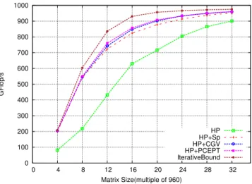
0 100 200 300 400 500 600 700 800 900 1000 0 4 8 12 16 20 24 28 32 GFlop/s Matrix Size(multiple of 960) HP HP+Sp HP+CGV HP+PCEPT IterativeBound
Figure 10. Performance with different HP schedulers.
Figure 10 shows the performance of most relevant HP variants proposed above. Large matrices have relatively more number of independent tasks at different execution points, which well suit to HP variants. That is why even baseline HP starts performing better as matrix size increases. HP+Sp performance indicates that spoliation rule is very useful when there are not enough number of independent tasks. Considering priority constraints with some relaxation (HP+PCEPT) improves performance for intermediate matri-ces and its performance is very near to iterative bound for large matrices, which indicates that HP+PCEPT manages priorities (critical tasks) and tasks heterogeneity in well manner.
D. Feasibility of the implementation of HP corrections The first implementation of HP proposed in [23] was implemented on top of StarPU following a twofold approach. The baseline version of HP was applied when enough ready tasks were available (HP was said to be in a steady state). When fewer tasks got in the system (HP was said to be in a critical state), CPU were prevented to execute long tasks in order to ensure a fine termination. The corrections proposed in the present study are much more advanced and we discuss here the feasibility of the implementation. These corrections rely on three ingredients: combining queues, performing spoliation and preemption. Modern runtime systems such as StarPU provide infrastructure for designing user-level scheduling algorithms. In particular, dealing with user-level queues is natural and combining their GPU view immediate. On the other hand, spoliation and preemption require to abort CPU tasks which is not supported in most state-of-the-art runtime systems. However, recent contributions have been proposed by the runtime community to perform forward recovery in the context of resilience [24]. This mechanism could be applied to recover an aborted task and thus perform spoliation or preemption. Alternatively, speculative scheduling using simulation at runtime could be employed [25].
VII. COMPARISON OF ALL THREE APPROACHES
In this Section, we propose to compare these three ap-proaches (static, heftp, and heteroPrio) in different cases: first with original execution timings as measured on the actual platform, then with perturbed timings which are constant throughout the execution (like in Section IV), and finally with perturbed timings within an execution.
A. Original timings 0 100 200 300 400 500 600 700 800 900 1000 0 4 8 12 16 20 24 28 32 GFlop/s Matrix Size(multiple of 960) SS+GS SS heftp+MMS heftp HP+PCEPT HP+Sp HP IterativeBound
Figure 11. Performance with different types of schedulers.
Figure 11 shows a comparison between the best variants of different schedulers. The static schedule is obtained with
these exact timings, which is why allowing movement of GEMM and SYRK tasks (SS+GS strategy) reduces the per-formance slightly in this case. On large matrices, computing the quality static schedule is very costly, and the CP formu-lation is only able to provide a low performance solution. For dynamic strategies, HP+PCEPT obtains consistently better performance than the best heftp variant (which is heftp+MMS), and both outperform the static schedule and obtain performance very close to the upper bound for large matrix sizes. On intermediate matrix sizes (12 or 16), all solutions are relatively farther from the bound, which may indicate that it would be possible to design stronger bounds. B. Perturbed timings
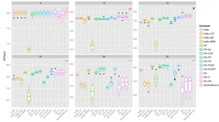
As indicated in Section IV, we consider 30 different sets of execution timings for each type of task on each resource, obtained by changing the original execution timings by ±10%. For consistency, these timings are then normalized to obtain the same area of the task graph as with original timings: all sets of execution timings for a particular matrix size will yield the same area bound. Unlike the previous case we provide here results about all variants discussed in the paper. Figure 12 shows the distribution of the performance of each algorithm for all matrix sizes, where plots are grouped by matrix sizes. For each matrix size and each algorithm, the box on the plot displays the median, first and last quartile, and the whiskers indicate minimum and maximum values, with outliers being shown as black dots.
Figure 12 shows that the performance of all HP variants increases with matrix size. It follows from the fact that HP variants are very good with a large number of independent heterogeneous tasks. The performance of heftp+LET and heftp+GBdegrade for large matrices due to their tendency to use the CPU resource greedily and thus allocate too many tasks which are well suited on GPU, as mentioned in Section V-B. As previously, the static solution is not very good for large matrices and most of the dynamic schedulers have better performance in these cases. However, we can also observe the benefits of dynamic modifications of this static solution, which allow to cope with perturbation of timings. As discussed in Section VI-B, the restrictive nature of the HP+PC scheduler yields a poor performance compared to other HP+Sp variants. On the other hand, its relaxed version HP+PCEPT achieves the best performance among all dynamic schedulers for intermediate and large matrices.
C. Perturbed timings within an execution
We now present the final set of experiments, in which ex-ecution timings for a particular task on a particular resource is not constant. Each time a task is executed, its execution timing is randomly drawn between ±10% of the original execution time. We ran our experiments with 30 different random seeds and show in Figure 13 the performance of
● ● ● ● ● ● ● ● ● ● ● ● ● ● ● ● ● ● ● ● ● ● ● ● ● ● ● ● ● ● ● ● ● ● ● ● ● ● ● 4 8 12 16 24 32 100 150 200 200 300 400 500 600 400 500 600 700 800 600 700 800 900 800 850 900 950 850 900 950 heftp heftp+LETheftp+GB heftp+MMS HP HP+Sp HP+CGVHP+PPHP+PCHP+PCEP HP+PCEPT SS SS+GSS+GS Iter ativ eBound heftp heftp+LETheftp+GB heftp+MMS HP HP+Sp HP+CGVHP+PPHP+PCHP+PCEP HP+PCEPT SS SS+GSS+GS Iter ativ eBound heftp heftp+LETheftp+GB heftp+MMS HP HP+Sp HP+CGVHP+PPHP+PCHP+PCEP HP+PCEPT SS SS+GSS+GS Iter ativ eBound GFlop/s Scheduler heftp heftp+LET heftp+GB heftp+MMS HP HP+Sp HP+CGV HP+PP HP+PC HP+PCEP HP+PCEPT SS SS+G SS+GS IterativeBound
Figure 12. Comparison of different schedulers with perturbed execution timings.
the best dynamic strategy and dynamic variants of static solutions for 12 × 12 matrix. This plot shows a behavior similar to other experiments for 12 × 12. It shows that even in this context, schedules based on the static solution always perform better than our best dynamic HeteroPrio scheduler (HP+PCEPT). It also shows that adding dynamic corrections to the static schedule tends to improve the overall performance in presence of perturbed timings.
12 740 750 760 770 780 SS SS+G SS+GS HP+PCEPT GFlop/s Scheduler SS SS+G SS+GS HP+PCEPT
Figure 13. Comparison of all SSbased strategies with best HP variant -12 × -12 tile matrix.
VIII. CONCLUSION AND PERSPECTIVES
This paper aims at providing a fair comparison between static and dynamic scheduling strategies on heterogeneous platforms consisting of CPU and GPU nodes. Runtime dynamic schedulers make their decisions based on the state of machine, on the set of available tasks and possibly on task priorities computed online. The success of these dy-namic strategies are motivated by expected weaknesses and limitations of static schedulers. First, it is well known that scheduling problems are hard (NP-Complete) and even hard to approximate with unrelated resources (what is the case in CPU-GPU platforms). Second, it has been observed that execution times of kernels in nodes where many resources (cache, memory, buses) are shared suffer high variance and it is generally assumed that the difficulty to predict execution times makes static schedulers useless. An original contribution of this paper is to prove that this last assertion is in general not true and that static schedules (for Cholesky factorization) are in fact robust to variations in execution times. On the other hand, the consequence of the greedy nature of basic dynamic strategies is that they make a poor use of "slow" resources like CPUs. Since the overall processing power of CPUs is in general small, this does not hurt too much the GFlop/s performance of kernels. Never-theless, we have proved that combining dynamic strategies with simulation in order to build less myopic algorithms
can significantly improve their performance. We have also considered a family of dynamic schedulers (HeteroPrio) that performs poorly on general graphs but greatly benefits from basic qualitative information about the task graph. Overall, this paper opens many perspectives. First, it advocates the design of efficient static schedules on heterogeneous unre-lated machines. Second, it advocates the introduction into dynamic schedulers of as much static knowledge about the application as possible in order to achieve good performance.
REFERENCES
[1] P. Brucker and S. Knust, “Complexity results for scheduling problems,” Web document, URL: http://www2.informatik.uni-osnabrueck.de/knust/class/.
[2] R. Bleuse, S. Kedad-Sidhoum, F. Monna, G. Mounié, and D. Trystram, “Scheduling independent tasks on multi-cores with gpu accelerators,” Concurrency and Computation:
Prac-tice and Experience, vol. 27, no. 6, pp. 1625–1638, 2015.
[3] C. Augonnet, S. Thibault, R. Namyst, and P.-A. Wacre-nier, “StarPU: A Unified Platform for Task Scheduling on Heterogeneous Multicore Architectures,” Concurrency and
Computation: Practice and Experience, Special Issue:
Euro-Par 2009, vol. 23, pp. 187–198, Feb. 2011.
[4] J. Planas, R. M. Badia, E. Ayguadé, and J. Labarta, “Hi-erarchical task-based programming with StarSs,”
Interna-tional Journal of High Performance Computing Applications,
vol. 23, no. 3, pp. 284–299, 2009.
[5] A. YarKhan, J. Kurzak, and J. Dongarra, QUARK Users’
Guide: QUeueing And Runtime for Kernels, UTK ICL, 2011.
[6] G. Bosilca, A. Bouteiller, A. Danalis, M. Faverge, T. Hérault, and J. Dongarra, “PaRSEC: A programming paradigm ex-ploiting heterogeneity for enhancing scalability,” Computing
in Science and Engineering, vol. 15, no. 6, 2013.
[7] H. Topcuoglu, S. Hariri, and M.-y. Wu, “Performance-effective and low-complexity task scheduling for heteroge-neous computing,” IEEE Transactions on Parallel and
Dis-tributed Systems, vol. 13, no. 3, pp. 260–274, 2002.
[8] A. Buttari, J. Langou, J. Kurzak, and J. Dongarra, “A class of parallel tiled linear algebra algorithms for multicore ar-chitectures,” Parallel Comput., vol. 35, pp. 38–53, January 2009.
[9] “PLASMA Users’ Guide, Parallel Linear Algebra Software for Multicore Architectures, Version 2.0,” http://icl.cs.utk.edu/plasma, University of Tennessee, November 2009.
[10] F. G. Van Zee, E. Chan, R. A. van de Geijn, E. S. Quintana-Orti, and G. Quintana-Quintana-Orti, “The libflame Library for Dense Matrix Computations,” Computing in Science and
Engineering, vol. 11, no. 6, pp. 56–63, Nov./Dec. 2009.
[11] E. Chan, F. G. V. Zee, P. Bientinesi, E. S. Quintana-Ortí, G. Quintana-Ortí, and R. A. van de Geijn, “Supermatrix: a multithreaded runtime scheduling system for algorithms-by-blocks,” in PPOPP, 2008, pp. 123–132.
[12] E. Agullo, C. Augonnet, J. Dongarra, H. Ltaief, R. Namyst, S. Thibault, and S. Tomov, “Faster, Cheaper, Better – a Hybridization Methodology to Develop Linear Algebra Software for GPUs,” in GPU Computing Gems. Morgan Kaufmann, 2010. [Online]. Available: http://hal.inria.fr/inria-00547847/en/
[13] G. Bosilca, A. Bouteiller, A. Danalis, M. Faverge, H. Haidar, T. Herault, J. Kurzak, J. Langou, P. Lemarinier, H. Ltaief, P. Luszczek, A. YarKhan, and J. Dongarra, “Distributed-Memory Task Execution and Dependence Tracking within DAGuE and the DPLASMA Project,” Innovative Computing
Laboratory Technical Report, 2010.
[14] “Chameleon, a dense linear algebra software for heterogeneous architectures,” 2014. [Online]. Available: https://project.inria.fr/chameleon
[15] H. Casanova, A. Legrand, and M. Quinson, “SimGrid: a Generic Framework for Large-Scale Distributed Experi-ments,” in 10th IEEE International Conference on Computer
Modeling and Simulation (UKSim), Apr. 2008.
[16] R. L. Graham, “Bounds on multiprocessing timing anoma-lies,” SIAM journal on Applied Mathematics, vol. 17, no. 2, pp. 416–429, 1969.
[17] H. Bouwmeester and J. Langou, “A critical path approach to analyzing parallelism of algorithmic variants. application to cholesky inversion,” CoRR, vol. abs/1010.2000, 2010. [Online]. Available: http://arxiv.org/abs/1010.2000
[18] H. M. Bouwmeester, “Tiled algorithms for matrix computa-tions on multicore architectures,” Ph.D. dissertation, Univer-sity of Colorado, Denver, 2012.
[19] R. D. Blumofe and C. E. Leiserson, “Scheduling multi-threaded computations by work stealing,” Journal of the ACM
(JACM), vol. 46, no. 5, pp. 720–748, 1999.
[20] P. Baptiste, C. Le Pape, and W. Nuijten, Constraint-based
scheduling: applying constraint programming to scheduling
problems. Springer Science & Business Media, 2012, vol. 39.
[21] A. Z. S. Shahul and O. Sinnen, “Scheduling task graphs optimally with a*,” The Journal of Supercomputing, vol. 51, no. 3, pp. 310–332, 2010.
[22] E. Agullo, O. Beaumont, L. Eyraud-Dubois, J. Herrmann, S. Kumar, L. Marchal, and S. Thibault, “Bridging the Gap between Performance and Bounds of Cholesky Factorization on Heterogeneous Platforms,” in HCW 2015, Hyderabad, India, 2015.
[23] E. Agullo, B. Bramas, O. Coulaud, E. Darve, M. Messner, and T. Takahashi, “Task-based FMM for multicore architectures,”
SIAM J. Scientific Computing, vol. 36, no. 1, 2014.
[24] L. Jaulmes, E. Ayguadé, M. Casas, J. Labarta, M. Moretó, and M. Valero, “Exploiting asynchrony from exact forward recovery for due in iterative solvers,” in SC ’15. New York, NY, USA: ACM, 2015, pp. 53:1–53:12.
[25] L. Stanisic, S. Thibault, A. Legrand, B. Videau, and J.-F. Méhaut, “Modeling and simulation of a dynamic task-based runtime system for heterogeneous multi-core architectures,” in Euro-Par 2014. Springer, 2014, pp. 50–62.