HAL Id: hal-02547692
https://hal.archives-ouvertes.fr/hal-02547692
Submitted on 20 Apr 2020
HAL is a multi-disciplinary open access
archive for the deposit and dissemination of
sci-entific research documents, whether they are
pub-lished or not. The documents may come from
teaching and research institutions in France or
abroad, or from public or private research centers.
L’archive ouverte pluridisciplinaire HAL, est
destinée au dépôt et à la diffusion de documents
scientifiques de niveau recherche, publiés ou non,
émanant des établissements d’enseignement et de
recherche français ou étrangers, des laboratoires
publics ou privés.
Martin Cooper, Simon de Givry, Thomas Schiex
To cite this version:
Martin Cooper, Simon de Givry, Thomas Schiex. Graphical Models: Queries, Complexity, Algorithms.
Leibniz International Proceedings in Informatics , Leibniz-Zentrum für Informatik, 2020, 154, pp.4:1–
4:22. �10.4230/LIPIcs.STACS.2020.4�. �hal-02547692�
Algorithms
Martin C. Cooper
Université Fédérale de Toulouse, ANITI, IRIT, Toulouse, France [email protected]
Simon de Givry
Université Fédérale de Toulouse, ANITI, INRAE, UR 875, Toulouse, France https://miat.inrae.fr/degivry/
Thomas Schiex
1Université Fédérale de Toulouse, ANITI, INRAE, UR 875, Toulouse, France http://www.inrae.fr/mia/T/schiex
[email protected] Abstract
Graphical models (GMs) define a family of mathematical models aimed at the concise description of multivariate functions using decomposability. We restrict ourselves to functions of discrete variables but try to cover a variety of models that are not always considered as “Graphical Models”, ranging from functions with Boolean variables and Boolean co-domain (used in automated reasoning) to functions over finite domain variables and integer or real co-domains (usual in machine learning and statistics). We use a simple algebraic semi-ring based framework for generality, define associated queries, relationships between graphical models, complexity results, and families of algorithms, with their associated guarantees.
2012 ACM Subject Classification Theory of computation → Discrete optimization; Mathematics of computing → Graph algorithms
Keywords and phrases Computational complexity, tree decomposition, graphical models, submodu-larity, message passing, local consistency, artificial intelligence, valued constraints, optimization Digital Object Identifier 10.4230/LIPIcs.STACS.2020.4
Category Tutorial
Supplement Material http://github.com/toulbar2/toulbar2
Funding The authors have received funding from the French “Investing for the Future – PIA3” program under the Grant agreement ANR-19-PI3A-000, in the context of the ANITI project. Martin C. Cooper : Funded by ANR-18-CE40-0011
Simon de Givry: Funded by ANR-16-CE40-0028. Thomas Schiex: Funded by ANR-16-CE40-0028.
1
Introduction
Graphical models are descriptions of decomposable multivariate functions. A variety of famous frameworks in Computer Science, Logic, Constraint Satisfaction/Programming, Machine Learning, Statistical Physics and Artificial Intelligence can be considered as specific sub-classes of graphical models. In this paper, we restrict ourselves to models describing functions of variables having each a finite (therefore discrete) domain with a totally ordered co-domain, that may be finite or not. This excludes, for example, “Gaussian Graphical Models” which are used in statistics, describing continuous probability densities.
1 Corresponding author
© Martin C. Cooper, Simon de Givry, and Thomas Schiex; licensed under Creative Commons License CC-BY
A graphical model over a set of variables is defined by a finite set of small functions which are combined together using a binary associative and commutative operator, defining a joint multivariate function. The combined functions may be small because they involve few variables or because they are described using a restricted language.
As an example, propositional logic (PL) is organized around the idea of describing logical properties as functions over Boolean variables. From the values of these variables, one should be able to determine if a property is true or not. A usual way to achieve this is to use clauses (disjunction of variables or their negation) as “small functions” and combine them with conjunction, defining the Conjunctive Normal Form. The resulting joint function defines the truth value of the formula. Various queries on such graphical models have been considered: existence of a variable assignment that optimizes the joint function, the SAT/PL problem, model counting (the #P-complete #-SAT/PL problem), etc.
If we instead use tensors to describe Boolean functions over sets of variables of bounded cardinality and combine these functions with conjunction again, we obtain a constraint network (CN) and the existence of an assignment that optimizes the joint function is the Constraint Satisfaction Problem (CSP/CN).
In the extreme, we may use tensors to describe small real (in R) functions combined using addition or multiplication, enabling the description of discrete probability distributions, as done with Markov Random Fields (MRFs) and Bayesian Networks (BNs) [74, 16]. The associated optimization problem is the Maximum A Posteriori (MAP/MRF) problem and weighted counting allows to compute the partition function [74] (or normalizing constant), another #P-complete problem with important applications in statistical physics and machine learning. The terminology of “graphical models” comes from the stochastic facet of GMs. Stochastic graphical models are of specific interest because they can be learned (or estimated) from data. Assuming that an i.i.d. sample of an unknown probably distribution is available, one may look for a graphical model that gives maximum probability to the sample. This maximum-likelihood approach has attractive asymptotic properties [74]. Efficient approximate estimation algorithms based on convex optimization exist [95]. Because of the unavoidable sampling noise, exact optimization algorithms are usually not sought. In this paper, we assume that the graphical models are known, either because they describe known rules or functions or have been previously estimated from data.
In this stochastic case, algorithms that provide some form of guarantee remain desirable, especially if the considered graphical model combines logical (deterministic) information, describing known/required properties, with probabilistic information learned from data. Indeed, logical information cannot be approximated without a complete loss of semantics.
In the rest of this paper, we first give an algebraic definition of what a graphical model is and consider the most usual queries. We then introduce the two main families of algorithms that can be used to exactly solve such queries: tree search and non-serial dynamic programming. Restricted to small sub-problems, we show how dynamic programming can provide fast approximate algorithms, called message-passing or local consistency enforcing algorithms, including associated polynomial classes. We then consider some empirically useful hybrid algorithms, with associated solvers, based on these approaches and recent applications in structural biology.
2
Notations, Definition
Variables are denoted as capital variables X, Y, Z, . . . that may be optionally indexed (Xi or
just i). Variables can be assigned values from their domain. The domain of a variable X is denoted as DX or Difor variable Xi. Actual values are represented as a, b, c, g, r, t, 1 . . .
and an unknown value denoted as u, v, w, x, y, z . . . . Sequences or sets of objects are denoted in bold. A sequence of variables is denoted as X, Y , Z, . . . A sequence of values is denoted as
u, v, w, x, y, z . . .. The domain of a sequence of variables X is denoted as DX, the Cartesian product of the domains of all the variables in X. An assignment uX is an element of DX which defines an assignment for all the variables in X. Finally, we denote by uX[Y ] (or uY) the projection of uX on Y ⊆ X: the sequence of values that the variables in Y takes in uX.
IDefinition 1 (Graphical Model). A Graphical Model M = hV , Φi with co-domain B and a
combination operator ⊕ is defined by:
a sequence of n variables V , each with an associated finite domain of size less then d. a set of e functions (or factors) Φ. Each function ϕS ∈ Φ is a function from DS → B.
S is called the scope of the function and |S| its arity.
M defines a joint function: ΦM(v) =
M
ϕS∈Φ
ϕS(v[S])
In this definition we assume that the co-domain B is totally ordered (by ≺) with a minimum and maximum element. Arbitrary elements of B will be denoted by Greek letters (α, β, . . .). The combination operator ⊕ is required to be associative, commutative, monotonic and has an identity element 0 ∈ B, the minimum element of B. The maximum element > of B is required to be absorbing (α ⊕ > = >). This set of axioms defines what is called a valuation structure [104], introduced in AI to represent graded beliefs or costs in Constraint Networks. It is closely related to triangular co-norms, often using B = [0, 1] [72]. It is also known as a tomonoid in algebra and includes tropical algebra [56]. Commutativity and associativity make the combination insensitive to the order of application of ⊕. Monotonicity captures the fact that adding more information can only strengthen it. Finally, the specific roles of the maximum and minimum elements of B are here to express deterministic information: 0 represents the fact that a function has reached an absolute minimum and this has no effect on the value of the joint function value Φ. Instead, any combined function taking value > will lead to a joint function that is also equal to >. For simplicity, we assume that elements of B can be represented in constant space and that a ⊕ b can be computed in constant time. An important additional property of ⊕ is often considered: idempotency (α ⊕ α = α). As section 6.1 will show, it has strong algorithmic implications. Finally, such valuation structures are said to be fair if, for any elements of B such that β4 α, there exists a maximum γ such that β ⊕ γ = α (such a γ may not exist in infinite structures). This element γ is denoted
α β and defines a pseudo-inverse operator (we have β ⊕ (α β) = α).
Table 1 Some valuation structures. Idemp. indicates the idempotency of ⊕. See [33] for details.
Structure (GM) B a ⊕ b ≺ 0 > Idemp. a b
Boolean (PL,CN) {t, f } a ∧ b t < f t f yes a
Additive (GAI) N¯ a + b < 0 +∞ no a − b
Weighted (CFN) {0,1, . . . , k} min(k, a+b) < 0 k no (a = k ? k : a−b) Probabilistic (MRF,BN) [0, 1] a × b > 1 0 no a/b Possibilistic (PCN) [0, 1] max(a, b) < 0 1 yes max(a, b) Fuzzy (FCN) [0, 1] min(a, b) > 1 0 yes min(a, b)
Valuation structures have been analyzed in detail [33, 31]. We know that any fair and countable valuation structure can be viewed as a stack of additive/weighted valuation structures, which interact with each other as an idempotent structure (thus using ⊕ = max).
The case ⊕ = max being very close to the case of classical Constraint Networks [88, page 293], most of the work has since then focused on the weighted and probabilistic cases.
The mathematical definition of graphical models above needs to be further refined by defining how the functions ϕS ∈ Φ are represented. Thanks to the assumption of finite domains, a universal representation of functions can be obtained using tensors (or multi-dimensional tables) that map any sequence of values uS ∈ DS to an element of B. This representation requires O(d|S|) space where d is the maximum domain size. When useful, alternative specialized representations may be used, with possibly different complexities for various elementary operations and queries.
Altogether, this definition of graphical models covers a variety of well-studied frameworks, including constraint networks [101] (tensors + Boolean), propositional logic [14] (Boolean domains, clauses + Boolean), generalized additive independence models [7] (tensors + addi-tive), weighted propositional logic (Boolean domains, clauses + addiaddi-tive), Markov Random Fields [71, 74] (tensors + Probabilistic), Bayesian networks [74] (MRFs with normalized tensors describing conditional probabilities, organized according to a directed acyclic graph), Possibilistic and Fuzzy Constraint Networks [48] (tensors + Possibilistic/Fuzzy). There are various related models, such as Ceteris Paribus networks (or CP-nets [47]) that could be covered using a weaker set of axioms, possibly too weak to prove interesting results.
We are biased in the paper towards the family of Cost Function Networks (CFN) which are GMs using tensors (extended with so-called “global functions”, see e.g. [81, 3]) and the Weighted structure. This combines the ability of combining additive finite weights with a finite upper bound cost that appears naturally in many situations.
I Definition 2. Two graphical models M = hV , Φi and M0 = hV , Φ0i, with the same
variables and valuation structure are equivalent iff they define the same joint function:
∀v ∈ DV, ΦM(v) = ΦM0(v).
CFNs have a tight relationship with stochastic graphical models. Since log(a × b) = log(a) + log(b), a −log transform applied to elements of B followed by suitable scaling, shifting and rounding can transform any stochastic graphical model into a Cost Function Network defining a joint function that represents a controlled approximation of the −log() of the joint function of the stochastic model. The function log being monotonic, MAP/MRF and WCSP/CFN are essentially the same problems.
IDefinition 3. Given two graphical models M = hV , Φi and M0= hV , Φ0i, with the same
variables and valuation structure, M is a relaxation of M0 iff ∀v ∈ DV, ΦM(v)4 ΦM0(v).
In a graphical model, the set of variables V and the set of scopes S of the different functions ϕS ∈ Φ define a hyper-graph whose vertices are the variables of V and the hyper-edges the different scopes. In the case in which the maximum arity is limited to 2, this hyper-graph is a graph, called the constraint graph or problem graph (hence the name graphical model). When larger arities are present, one can use the 2-section of the hypergraph as an approximation of it, often called the primal or moral graph of the GM. The bipartite incidence graph of this hypergraph has elements of V and Φ as vertices, an edge connecting
X ∈ V to ϕS iff X ∈ S and is often called the factor graph [1] of the graphical model. This hyper-graph or its incidence graph only captures the overall structure of the model but neither the domains nor the functions. Therefore, a more fine-grained representation, known as the micro-structure graph, is often used to represent (pairwise) graphical models, vertices representing values and weighted edges the value of functions on pairs of values.
3
Queries
A query over a graphical model asks to compute simple statistics over the function such as its minimum or average value. Such queries already cover a wide range of practical usages. Assuming that true ≺ false, the SAT/PL [14] and CSP/CN [101] problems are equivalent to finding the minimum of the joint function, which is also the case for (Weighted) Max-SAT, WCSP/CFN, MAP/MRF (or MPE/BN aka Maximum Probability Explanation in Bayesian Networks). In these optimization problems, we want to compute minv∈DV Φ(v). Alternatively, for numerical B, counting problems require to compute
P
v∈DV Φ(v). A relatively general situation can be captured by introducing a so-called
“elimination” operator ⊗, assumed to be associative, commutative and such that ⊕ distributes over ⊗: α ⊕ (β ⊗ γ) = (α ⊕ β) ⊗ (α ⊕ γ). The two operations (⊗, ⊕) and their associated properties have been studied, with some variations, under a variety of names, often in relation with non-serial dynamic programming [110, 17, 1, 73, 72, 56]. The query to answer becomes N
v∈DV ⊕ϕS∈ΦϕS(v[S]).
A powerful toolbox on graphical models can be built from three simple operations: assignment (or conditioning), combination and elimination.
Given a function ϕS, it is possible to assign a variable Xi ∈ S with a value a ∈ Di. We
obtain a function on T = S − {Xi} defined by ϕT(v) = ϕS(v ∪ {Xi= a}). If we assign all
the variables of a function, we obtain a function with an empty scope, denoted ϕ∅. This operation has negligible complexity (we directly access a part of the original cost function).
The second operation is the equivalent of the relational join operation in databases: it combines two functions ϕS and ϕS0 into a single function, which is equivalent to their
combination by ⊕. The resulting function has the scope S ∪ S0 and is defined by (ϕS⊕
ϕS0)(v) = ϕS(v[S]) ⊕ ϕS0(v[S0]). The calculation of the combination of the two functions is
exponential in time and space (O(d|S∪S0|)). Observe that we can replace a set of functions by their combination without changing the joint function defined by the graphical model (preserving equivalence).
Finally, the elimination operation consists in summarising the information from a function
ϕS on a subset of variables T ⊂ S. The elimination of the variables of S − T in ϕS leads to its so-called projection (or marginal) onto T , the function ϕT(u) =Nv∈DS−T ϕS(u ∪ v).
Since elimination requires enumerating the whole domain DS of ϕS, it has time complexity
O(d|S|). The resulting function requires O(d|T |) space. If S − T is a singleton {Xi}, we will
denote by ϕS[−Xi] = ϕS[S − {Xi}] the result of the elimination of the single variable Xi.
These complexities are given for functions represented as tensors. They may change if other languages such as clauses, analytic representation or compact data structures such as weighted automata or decision diagrams [38, 51] are used to represent functions.
We close this section by expressing simple graph problems as WCSP/CFNs.
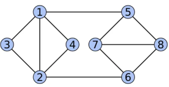
Given an undirected graph G = hV , Ei with vertex set V and edge set E, we can define the following WCSP/CFN M = hV , Φi problems, having one variable per vertex:
s−t Min-Cut: ∀i ∈ V \{s, t}, Di= {a, b}, Ds= {a}, Dt= {b}, and Φ = {ϕij| (i, j) ∈ E},
with ϕij(a, a) = ϕij(b, b) = 0 and ϕij(a, b) = ϕij(b, a) = 1.
Max-Cut: ∀i ∈ V , Di= {a, b}, Φ = {ϕij | (i, j) ∈ E}, with ϕij(a, a) = ϕij(b, b) = 1 and
ϕij(a, b) = ϕij(b, a) = 0.
Vertex Cover: ∀i ∈ V , Di= {a, b}, Φ = {ϕi| i ∈ V }S{ϕij | (i, j) ∈ E}, with ϕi(a) = 0,
ϕi(b) = 1, ϕij(a, b) = ϕij(b, a) = ϕij(b, b) = 0 and ϕij(a, a) = >.
Max-Clique: ∀i ∈ V , Di= {a, b}, Φ = {ϕi| i ∈ V }S{ϕij | (i, j) 6∈ E}, with ϕi(a) = 0,
2
4
3
1
5
7
8
6
Figure 1 Simple graph example (from Wikipedia DSATUR). Optimum value and corresponding solution for Min-Cut (s = 1, t = 8): ΦM(aaaabbbb) = 2, Max-Cut: ΦM(aabbbbaa) = 2 (i.e., a maximum
cut involving 12−2 = 10 edges), Vertex Cover: ΦM(bbaaaabb) = 4, Max-Clique: ΦM(aaabbbbb) = 5
(i.e., a maximum clique of size 8−5 = 3), 3-Coloring: ΦM(abccccab) = 0, and Min-Sum 3-Coloring:
ΦM(bcaaaabc) = 14.
Graph Coloring with 3 colors: ∀i ∈ V , Di= {a, b, c}, Φ = {ϕij | (i, j) ∈ E}, with ∀u, v,
ϕij(u, v) = 0 if u 6= v and ϕij(u, v) = > otherwise.
Min-Sum Coloring with 3 colors: ∀i ∈ V , Di = {a, b, c}, Φ = {ϕi | i ∈ V }S{ϕij |
(i, j) ∈ E}, with ϕi(a) = 1, ϕi(b) = 2, ϕi(c) = 3, and ∀u, v, ϕij(u, v) = 0 if u 6= v and
ϕij(u, v) = > otherwise.
An example of optimal solution for each problem is given in Fig.1.
4
Tree search
One of the most basic algorithms to answer the queryN
v∈DV ⊕ϕS∈Φrelies on conditioning
and can be described as brute force tree-search. It relies on the fact that if all variables in a graphical model are assigned (all variables have domain size 1), the answer can be obtained by just computing Φ on the assignment. If a given model has a variable Xi∈ V with a larger
domain, the query can be reduced to solving two queries on simpler models, one where Xi is
assigned to some value a ∈ Diand the other where a is removed from Di. The result of these
queries is then combined using ⊗. This can be understood as the exploration of a binary tree whose root is the original graphical model and where leaves are fully assigned models on which the query can be answered. This tree can be explored using various strategies (Depth-First, Breadth-First, Iterative [94],. . . ), DFS has O(nd) space and θ(exp(n)) time.
In the case of optimization (⊗ = min) on a GM M it is possible to exploit any available lower bound on the values of the leaves below a given node in the tree for pruning. If this lower bound is larger than or equal to the value of the joint function on a best known leaf, then the sub-tree can be pruned. If M contains a constant function ϕ∅ with empty scope, then the value of this function provides such a lower bound, thanks to monotonicity and non-negativity. With pruning, the order in which this tree is explored (the choice of the branching variable Xi and value a) becomes crucial for empirical efficiency.
5
Non-serial Dynamic Programming
An alternative approach for answering the query above consists in using non-serial dynamic programming (DP) [11], also called Variable-Elimination (VE), bucket elimination [44], among other names [74, 110, 1]. The process relies on the distributivity of ⊗ over ⊕ and has also been described as the Generalized Distributive Law[1]. To our knowledge, its axiomatic requirements in a general situation were first studied in [110]. The fundamental idea itself is reminiscent of famous elimination algorithms (e.g. Gaussian elimination) and was already
described in 1972 under the name of Non-Serial Dynamic Programming [11], which we use. This book also defines a graph parameter (Dimension), and is the same as tree-width [19]. In its simplest variable elimination variant, non serial DP works variable per variable, replacing a variable X and all functions that involve it by a function on the neighbors of
X. Following the stochastic GMs terminology, this new function will be called a “message”.
Given a graphical model M = hV , Φi, a variable X ∈ V , let ΦX be the set of functions
ϕS∈ Φ such that X ∈ S and T the neighbors of X in the graph of the problem, we define the message mΦX T from ΦX to T as: mΦX T = ( M ϕS∈ΦX ϕS)[−X] (1)
By distributivity, it is now possible to rewrite our query as: O v∈DV ⊕ ϕS∈Φ ϕS(v[S]) = O v∈DV −{X} ⊕ ϕS∈Φ−ΦX∪{mΦXT } ϕS(v[S])
This equality shows that our initial query can be answered by solving a similar query on a graphical model that has one variable less and where all functions involving this variable have been replaced by a new function (or message) mΦTX. This operation can be applied to every variable successively until a final graphical model with no variable and a constant function ϕ∅ is obtained. The value of this function is the answer to the initial query.
When tensors are used to represent functions, the successive applications of combination and elimination show that computing mXT is O(d|T +1|) time and space but space can be easily reduced to O(d|T |) if elimination is performed incrementally. This can be different with other representations. In propositional logic, if ` is a literal over variable X and if ΦX contains the two clauses ϕS= (` ∨ L) and ϕS0 = (¬` ∨ L0), where L and L0are clauses, then
the message mX
T obtained by combining the two clauses and eliminating X is the function represented by the clause L ∨ L0: the resolution principle [99] performs efficient variable elimination [45].
It is well-known that the order in which the variables are eliminated can have a strong influence on the complexity of the whole process. Each elimination creates a new function whose scope is known. As each step is exponential in the number of variables in the neighbourhood of the eliminated variable X which come after X in the elimination order, one may prefer to simulate the process (play the elimination game) and get an estimate of the global complexity without actually performing the calculations. It is the step for which the number w of future neighbors is maximum which determines the complexity (spatial and temporal): this complexity is exponential in w. The parameter w is called the induced width of the graph of the GM but is better known as its tree-width for the given elimination order. Minimizing w is known to be NP-hard, but useful heuristics exist [18].
This algorithm defines the first non-trivial tractable class for the query above: graphical models with a bounded tree-width graph.
5.1
Message passing
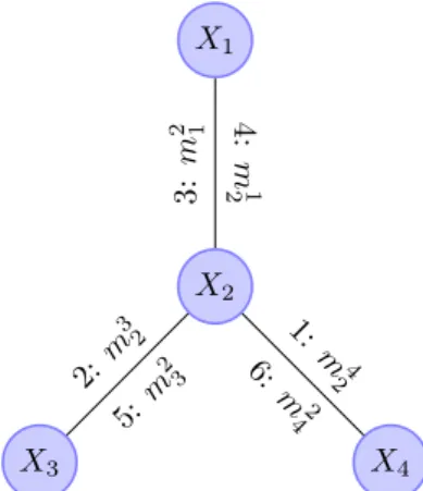
The bounded tree-width class is specifically interesting for pairwise models M with an acyclic graph (tree-width one). In this case, the query above can be solved by rooting the tree in any variable X ∈ V and iteratively eliminating the leaves of this graph until only the root remains. In this case, messages mX
X1 X2 X3 X4 3: m 2 1 4: m 1 2 2:m 3 2 5:m 2 3 1: m4 2 6: m2 4
Figure 2 The graph of a GM with three pairwise functions. The marginal of Φ on X2 can be
computed by combining all three incoming messages: m32, m 1 2, m
4 2.
to the elimination of variable Xi with parent Xj through edge ϕij is just denoted mij (a
message from i to j). Denoting by neigh(X) the set of neighbor variables of X in the tree, the message computed by applying Eq. 1 is:
mij = ⊗
Xi
(ϕi⊕ ϕij ⊕ Xo∈neigh(Xi),o6=j
moi)
In the end, one variable X remains and the joint function Φ it defines describes the so-called marginal of the joint function defined by M. This is a function of X that answers the query for every possible assignment of X.
These marginal functions are of specific interest in counting queries over stochastic models as they provide marginal probabilities. Specific algorithms have therefore been developed to compute the marginals over all the variables of acyclic models. This requires only two steps (instead of one per variable). In this algorithm, messages are computed and kept aside and no function is removed from the graphical model. We therefore have an initially empty, growing list L of computed messages. If a variable has received messages from all its neighbors but one, it becomes capable of computing the message for this variable and adds it to the list of computed messages. The algorithm therefore starts by computing messages from leaves and ultimately computes two messages mij and mji for every edge ϕij. For any variable Xi, the
marginal of the joint function Φ on Xi is directly accessible as ϕi⊕o∈neigh(Xi)m o
i. It is easy
to check that the gathered messages for every vertex X are exactly those that would have been done if the tree had been rooted in X.
If the initial graph is cyclic, a tree decomposition of the graph can be identified and the algorithm above used to send messages mC
S by combining all functions in cluster C and projecting to separator S. The resulting algorithms similarly computes marginals over clusters which can be further projected onto every variable inside [74]. This has two advantages over the pure variable elimination algorithm above: the space complexity is
O(exp(s)) where s is the size of the largest separator in the tree decomposition and all the
marginals are accessible. In its “one-pass” variant, this algorithm is the “block-by-block” elimination introduced in 1972 by Bertelé and Brioschi [11]. Despite the improved space complexity (but unchanged time complexity), this algorithm is restricted to problems with very small tree-width (especially with large domain sizes).
6
Loopy Belief propagation and Local Consistency
The Loopy Belief Propagation heuristic can be used when the algorithm above cannot finish in reasonable time. In a pairwise model, the list L is initialized with all possible constant empty messages mji = mij = 0 for all ϕij ∈ Φ. Every message is then updated using the
same equation as above: mi
j = ⊗Xi(ϕi⊕ ϕij⊕Xo∈neigh(Xi),o6=jm o
i). These updates can be
done synchronously (new versions are all computed simultaneously and replace those of the previous iteration) or asynchronously. This is repeated until quiescence or after a finite number of iterations as the algorithm has no guarantee of termination in general. Loopy BP was introduced by Pearl [96] and later used for signal coding and encoding defining Turbo-decoding [10]. Despite its limited theoretical properties, it is one of the most used algorithms over stochastic graphical models, probably the most cited (implemented in every GSM phone). It has been the object of intense study [117]. It can be used to get heuristic answers for optimization or counting queries under the name of the max-sum, min-sum or sum-prod algorithm [1].
6.1
Local consistency and Filtering
For optimization (⊗ = min), if ⊕ is either idempotent or fair, these algorithms can be transformed into well-behaved polytime reformulation techniques that provide incremental lower bounds, for Branch and Bound algorithms.
ITheorem 4. Suppose that ⊕ is idempotent, and consider M = hV , Φi and M0 = hV , Φ0i
a relaxation of M. Then M00= hV , Φ ∪ Φ0i is equivalent to M.
Proof. From the axioms of an idempotent valuation structure, consider two valuations
04 β 4 α ∈ B. Then α = α ⊕ 0 4 α ⊕ β 4 α ⊕ α = α by identity, monotonicity and idempotency successively. Then ΦM00= ΦM⊕ ΦM0. The results follows from the fact that
M0 is a relaxation of M.
J ITheorem 5. If ⊗ = min, any message mX
T computed by elimination is a relaxation of ΦX
and therefore of M.
This follows directly from the definition of a message and the fact that ⊗ = min. Together, these results show that any message (computed by Eq. 1) can be added to an idempotent graphical model, without changing its meaning. This result applies to the Boolean, Possibilistic and Fuzzy cases. In the Boolean case, we recover the trivial fact that a logical consequence (relaxation) of a formula can be added to it without changing its semantics (as achieved by the resolution principle [99] and the seminal Davis and Putnam algorithm [40]). It also immediately provides algorithms for Possibilistic and Fuzzy graphical models [49].
These observations are very useful in the context of message passing algorithms. If ⊕ is idempotent, it becomes possible to add the generated messages to the set of functions Φ of the graphical model with the guarantee that equivalence will be preserved. This idea underlies all the “(Boolean) constraint propagation” algorithms (e.g., unit propagation in PL and arc consistency filtering in CNs) that have been actively developed in the last decades. We now give a non-standard definition of Arc Consistency in binary idempotent graphical models to illustrate this:
IDefinition 6. A graphical model M = hV , Φi with idempotent ⊕ is arc-consistent iff every
variable X ∈ V is arc consistent w.r.t. every function ϕS s.t. X ∈ S. A variable Xi is
arc-consistent w.r.t. a function ϕij iff the message m j
This local consistency property can be satisfied (or not) by an idempotent graphical model. When it’s not satisfied, there is an obvious brute force algorithm that can transform the non AC model into an equivalent AC model: it suffices to apply message passing and directly combine all messages mji in M until the ϕido not change. One can show that this algorithm
must stop in polytime and that the process is confluent (there is only one fixpoint). This algorithm is not optimal however and several generations of AC algorithms for e.g. Constraint Networks have been proposed until the first time optimal algorithm (AC4 [89]), the first space and time optimal (AC6 [13]) and the simplest empirically most efficient time/space optimal variant (AC2001 aka AC3.1) came out [12, 118].
Arc consistency and Unit Propagation in SAT are fundamental in efficient CSP and SAT provers. Adding messages (new unary functions) to the problem makes these unary functions increasingly tight. Ultimately, it may be the case that some ϕi∈ Φ becomes such
that ∀a ∈ Di, ϕi(a) = >. Because equivalence is preserved, it is then known that the joint
function of the original graphical model is always equal to > (it is inconsistent in logical terminology). Naturally, being a polytime process, arc consistency enforcing cannot provide such an inconsistency proof in all cases (assuming P 6= NP). Stronger, more expensive, messages can be obtained using messages mC
T combining functions in C projected onto
T . In pairwise GMs, when C is defined by all functions whose scope is included in any
set of cardinality less than i projected on any sub-scope of cardinality i − 1, this is called
i-consistency enforcing [30, 5], which solves idempotent GMs with tree-width less than i in
polynomial time.
6.2
The non idempotent fair case
When optimizing, if ⊕ is not idempotent, it becomes impossible to simply add messages to the graphical model being processed and preserve equivalence. However, the pseudo-difference operator of fair structures makes it possible to add the message to the model and compensate for this by subtracting the message from its source [103]. Such a generalization may lead to loss of guaranteed termination since information can both increase and decrease at different local levels. While usual local consistency enforcing takes a set of functions and adds the message m obtained by eliminating a subset of variables in the problem, what has been called an Equivalence Preserving Transformation (EPT) combines a set of functions into a new function ϕ, computes the associated message (or any relaxation of it) and replaces the original set of functions by m and ϕ m. When scopes are unchanged, this has been called reparameterizations in MRFs [115].
If the problem of computing an optimal sequence of EPTs (in the sense that applying these messages reformulate the GM into another one that has a maximum ϕ∅) is NP-hard for integer costs, finding an optimal set of messages using rational costs can be reduced to a linear programming instance of polynomial size [32], a reduction which was previously published in 1976 [109], in Russian. Schlesinger’s team has produced a variety of results on GMs that have been reviewed in English [116]. The LP-based algorithm has the ability to exactly optimize additive or weighted [29] GMs with a tree-structure or with only submodular functions but solving the LP is empirically too slow to be of practical use in most cases. This LP has been shown to be universal, in the sense that any reasonable LP can be reduced to (the dual of) such an LP in linear time, with a constructive proof [97].
IDefinition 7. Function ϕSis submodular if ∀u, v ∈ DS, ϕS(min(u, v)) + ϕS(max(u, v)) ≤
This assumes that domains are ordered, max and min being applied pointwise. If it exists, a witness order for submodularity can be easily found [108] defining the polynomial class of weighted GMs with permutated submodular functions [107].
The best known general algorithm for Boolean submodular function minimization is
O(en3logO(1)n) [82]. For CFNs, practical algorithms can be obtained by exploiting a
connection with idempotent GMs (here CNs). Any weighted function ϕS can be transformed into a Boolean function Bool(ϕS) which is true iff ϕS is non 0.
I Definition 8 ([34, 29]). Given a weighted GM (or CFN) M = hV , Φi, Bool(M) = hV , {Bool(ϕS) | |S| > 0}) (a constraint network).
IDefinition 9 (Virtual Arc Consistency (VAC)[34]). A weighted GM M = hV , Φi is Virtual
Arc Consistent iff enforcing AC on Bool(M) does not prove inconsistency.
If enforcing AC on Bool(M) yields an inconsistency proof, it is possible to extract a minimal sub-proof and transform it in a set of EPTs that will increase ϕ∅ when applied on M. The repeated application of this principle leads to an O(ed2m/ε) time, O(ed) space VAC
enforcing algorithm (where ε is a required precision). It can be seen as a sophistication of max-flow algorithms using “augmenting proofs” [77, 116]. On Min-Cut problems, proofs can have the expected augmenting path structure. Related algorithms, using a Block Coordinate Descent approach to approximately solve the LP above have also been investigated in Image processing: the TRW-S algorithm [75] fixpoints satisfy the VAC property (called Weak Tree Agreement in MRFs) which can be exploited to detect strongly persistent assignments [57] (subsets of variables having the same value in all optimal solutions). On GMs with Boolean variables, the bound ϕ∅ is related to the max-flow roof-dual lower bound of Quadratic Pseudo-Boolean Optimization [20].
All these algorithms ultimately produce strengthened lower-bounds ϕ∅. In the con-text of Branch & Bound, looser approximations of the dual are often used because of their high incrementality. One of the most useful is existential directional arc consistency, with O(ed2max(nd, m)), O(nd) space complexity on pairwise models [80], that solves
tree-structured problems.
7
Hybrid algorithms
In this section, we rapidly review a subset of the large number of hybrid algorithms that have been designed to rigorously answer optimization queries over graphical models. The arena of existing algorithms is currently clearly dominated by a family of algorithms that combines tree search with local consistency enforcing. Local consistency enforcing strengthens the obvious lower bound defined by ϕ∅. It reformulates the graphical model associated with each node of the search-tree incrementally. It provides improved information with tightened unary ϕi. This information can be used in cheap variable and value ordering heuristics, to
decide which variable to explore first, along which value. These heuristics are crucial for the empirical efficiency of the algorithms (as evaluated on large sets of benchmarks, which are increasingly available in this data era). They have have become adaptive [90, 21]: they are parameterized and these parameters change during tree search, trying to identify and favor the selection of variables that belong to the regions of the graphical model that contain strong information, variables which once assigned would lead to rapid backtracking.
These algorithms can be (empirically) enhanced by hybrid branching strategies mixing depth and best-first, restarts (preserving information not invalidated by restart), stronger message passing at the root node, dominance analysis (showing a value a can always be replaced by value b without degrading Φ allows us to remove a).
In the idempotent ⊕ case, conflict analysis [15] is a powerful technique that allows to produce a new informative relaxation (or logical consequence) of the model when a conflict occurs during tree search (a backtrack must occur). Initially developed [42] and improved [106] for Constraint Networks, this has been adapted to SAT and is now a fundamental ingredient of the modern CDCL (Conflict Directed Clause Learning) SAT provers that obsoleted the 90’s generation of advanced DPLL (Davis, Putnam, Logemann, Loveland) provers [39].
At this point, one may note that for optimization at least, the empirically most efficient algorithms are algorithms that have O(exp(n)) worst-case complexity while algorithms with better worst-case complexity (based on non-serial dynamic programming) are restricted to a small subset of problems having (small) bounded tree-width (depending on d). A series of proposals tried to define algorithms that combined the empirical efficiency of enhanced tree-search algorithms with tree-width based bounds. To the best of our knowledge, the first algorithm along this line is the Pseudo-Tree search algorithm [53], for solving the CSP in constraint networks. Defined in 1985, this algorithm relies on a so-called pseudo-tree (defined below). It is shown to have a complexity which is exponential in the height of the pseudo-tree and uses only linear space. This pseudo-tree height was later shown to be related by a log(n) factor to induced width (a synonymous of tree-width) in 1995 [9, 105]. Pseudo-tree height seems to be the exact equivalent of tree-depth [92].
IDefinition 10 (pseudo-tree, pseudo-tree height [53]). A pseudo-tree arrangement of a graph
G is a rooted tree with the same vertices as G and the property that adjacent vertices in G reside in the same branch of the tree. The pseudo-tree height of G is the minimum, over all pseudo-tree arrangements of G of the height of the pseudo-tree arrangement.
The idea was revived in the context of counting problems in the “Recursive Conditioning” algorithm, relying on the related notion of d-tree [37]. This was quickly followed by the proposal of two algorithms for CSP/CN, WCSP/CFN and MAP/MRF relying either on pseudo-trees, leading to the family of AND-OR tree and graph search algorithms [84, 86, 85, 87] or tree-decompositions, leading to the Backtrack Tree-Decomposition algorithm (BTD [66, 67, 41]) . These algorithms enhance the original pseudo-tree search along two lines: they add some form of local consistency enforcing to prune the search tree, with associated non trivial per-cluster lower-bound management and may also memorize information, leading to algorithms with worst-case time/space complexity that reach those of the best elimination algorithms, with much better empirical complexity, thanks to pruning and variable ordering heuristics.
These algorithms take as input a graphical model (we assume a pairwise GM for simplicity) and a tree decomposition of its graph. The tree decomposition is rooted in a chosen cluster. Then a usual (hybrid) tree-search algorithm is used but the variable assignment order is constrained by a rule that forbids to assign a variable from a cluster if all the variables of its parent cluster have not already been assigned. When this happens, the variables in the separators between the parent cluster and any of its sons are assigned: the functions that connect the parent and son clusters can be cheaply eliminated, the clusters disconnect and can be solved independently given the current assignment of the separator. This principle is applied recursively on sub-problems. For every first visit of a given assignment of a separator, it is possible to memorize the value of the query for this assignment. When the same assignment is revisited later, it can be directly reused. This is what the AND/OR graph search and BTD algorithms do, at the cost of an O(ds) space complexity. Their time
complexity, in the simplest case of the CSP problem, is just exponential in the tree-width instead of the pseudo-tree height. Alternatively, no space is used in the AND/OR tree search algorithm and the worst-case space and time complexity become those of the Pseudo-Tree Search algorithm (but with improved empirical complexity thanks to mini-bucket elimination, a specific form of message passing that provides the bounds required for pruning [43, 46]).
Thanks to the bounds and reformulations provided by local consistency enforcing, these algorithms will typically explore a tiny fraction of the separators, empirically requiring much less space than a pure non-serial dynamic programming algorithm. The constraint that the rooted tree decomposition imposes on variable assignment ordering will however play a possibly negative role. Finally, because space is an abrupt constraint in practice, tree-decompositions with large separators may be unexploitable in practice if a space-intensive approach is used. One usual way to deal with space constraints is to use a bounded amount of space for caching separator assignments and corresponding query answers and have some dedicated cache management strategy. In the end, the best tree-decompositions for hybrid algorithms such as BTD or Pseudo-Tree Search will usually not be minimum tree-width decompositions (if they could be computed). The usual approach here is to rely on simple heuristics such as min-degree, Maximum Cardinality Search [100] or min-fill to heuristically build a decomposition. This may be randomized and iterated [70]. The result may then be improved by cluster-merging operations, trying to minimize separator sizes while preserving sufficient cluster size so that variable ordering heuristics do not get too constrained. Not only we do not have any final definition of what is an optimal tree decomposition but even a simple min-fill heuristics may be too long in practice to be useful (on large GMs, executing the polytime min-fill algorithm on the GM graph may take more time than solving the later NP-hard query on the GM). For this reason, new approaches that directly and efficiently build empirically useful decompositions for GM optimization queries are now being introduced [64, 63]. To better exploit the fact that different assignments may lead to different subproblems, with different graphs at the micro-structure level, dynamic decomposition is also explored. Some of these strategies rely on iterated (hyper)graph-partitioning using large-graphs dedicated heuristics such as Metis [69] or PaToH [24, 79], in the spirit of the seminal Nested Dissection algorithm [54].
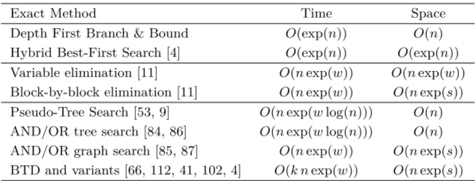
Table 2 Time and space complexities of exact methods for a CFN with tree-width w, s maximum separator size (s ≤ w ≤ n), and initial problem upper bound k.
Exact Method Time Space
Depth First Branch & Bound O(exp(n)) O(n) Hybrid Best-First Search [4] O(exp(n)) O(exp(n)) Variable elimination [11] O(n exp(w)) O(n exp(w)) Block-by-block elimination [11] O(n exp(w)) O(n exp(s)) Pseudo-Tree Search [53, 9] O(n exp(w log(n))) O(n) AND/OR tree search [84, 86] O(n exp(w log(n))) O(n) AND/OR graph search [85, 87] O(n exp(w)) O(n exp(s)) BTD and variants [66, 112, 41, 102, 4] O(k n exp(w)) O(n exp(s))
In the idempotent cases, the exploitation of tree-decompositions is implicit in algorithms relying on a combination of clause/constraint learning and restarts (confirmed in practice [62]).
ITheorem 11 ([6, 62]). A standard randomized CDCL SAT-solver with a suitable learning
strategy will decide the consistency of any pairwise Constraint Network instance with tree-width w with O(n2wd2w) expected restarts.
8
Additional complexity results
Although NP-hard in general, under certain restrictions, calculating the global value of a GM can be achieved in polynomial time. We have seen that this is the case when the tree-width of the primal graph is bounded by a constant. In terms of graph structure, the family of GMs
with bounded tree-width has been clearly the most exploited in practice (with the closely related branch-width [98]). In the non-pairwise case, parameters such as hypertree-width are implicitly exploited by hybrid algorithms such as BTD [65].
In the case of CFNs, restrictions on the language of cost functions can also define tractable classes. Restrictions which are not exclusively concerned with the graph, nor exclusively concerned with the language of cost functions define what are known as hybrid classes. We consider language-based tractable classes first.
The characterisation of all tractable languages of cost functions was a long-standing problem which has recently been solved thanks to the characterisation of tractable languages in the last remaining (and most difficult) case of Boolean valuation structures [22, 119]. This latter result resolved positively the so-called Feder and Vardi Conjecture [52] that there is a P/NP-complete dichotomy for the constraint satisfaction problem parameterized by the language of possible constraint relations [23].
There is only one non-trivial class of cost functions defining a tractable subproblem of CFNs which comes out of the study of Max-SAT: the class of submodular functions (see Definition 7). The class of submodular functions includes all unary functions, the binary functionspx2+ y2, ((x ≥ y)?(x − y)t: k) (for t ≥ 1), K − xy, the cut function of a graph and
the rank function of a matroid [55]. Efficient algorithms have been developed in Operations Research to minimize submodular functions [82, 25]. Another approach [34] consists in establishing virtual arc consistency (which preserves the submodularity of the cost functions). By the definition of VAC, the arc-consistency closure Q of Bool(P) is non-empty and, by definition of submodularity, its cost functions are both min-closed and max-closed [61]; to find a solution of Q (which is necessarily an optimal solution of P), it suffices to assign always the minimum (or always the maximum) value in each domain of Q.
A CFN can be coded as an integer programming problem (whose variables include
via∈ {0, 1} which is equal to 1 if and only if Xi= a in the original CFN instance [60]). The
linear relaxation of this integer programming problem (in which viais now a real number
in the interval [0, 1]) has integer optimal solutions if all cost functions are submodular, meaning that the CFN can be solved by linear programming. The dual of this relaxation is exactly the linear program used by OSAC [29] to find an optimal transformation (set of EPTs) [116]. CFNs restricted to a language of finite-valued cost functions over the valuation structure Q≥0∪ {∞} is tractable if and only if it is solved by this linear program [113]. This notably includes languages of cost functions that are submodular on arbitrary lattices. State-of-the-art results concerning the tractability of languages of cost functions are covered in detail in a recent survey article [78].
These theoretical results demonstrate the importance of submodularity and linear pro-gramming in the search for tractable subproblems of the CFN. However, we should mention that there are tractable languages of cost functions other than the class of submodular func-tions. For example, replacing the functions min and max in the definition of submodularity by any pair of commutative conservative functions f, g (where conservative means that ∀x, y,
f (x, y), g(x, y) ∈ {x, y}) gives rise to a tractable class [28].
Hybrid classes [36] may be defined by restrictions on the micro-structure of the CFN. To
illustrate this, we describe the hybrid tractable class defined by the joint winner property (JWP) [35]. A class of binary CFNs satisfies the JWP if for any three variable-value assignments (to three distinct variables), the multiset of pairwise costs imposed by the binary cost functions does not have a unique minimum. If there is no cost function explicitly defined on a pair of variables, then it is considered to be a constant-0 binary cost function. Note that the unary cost functions in a CFN that satisfies the JWP can be arbitrary. It has been
shown that there is a close link between the JWP and M]-convex functions studied in [91]. Indeed, a function satisfying the JWP can be transformed into a function represented as the sum of two quadratic M-convex functions, which can be minimized in polynomial time via an M-convex intersection algorithm. This leads to a larger tractable class of binary finite-valued CFNs, which properly contains the JWP class [59].
9
Solvers and applications
Thanks to a simple algebraic formulation of graphical models and queries over GMs, this review covers a very large variety of algorithms and approaches that have been developed in probabilistic reasoning, propositional logic and constraint programming. On the non stochastic side, SAT and CSP solvers have had a significant impact in several areas such as Electronic Design Automation (where SAT solvers are used as oracles to solve complex Bounded Model Checking problems), Software Verification (where suitable Abstraction Refinement Strategies are used to manage possibly very large instances [27, 58]) or for task scheduling [8] or planning [114] among many others. Stochastic variants are one of many modeling tools available in Machine Learning [16], but Markov Random Fields have been more specifically applied in Image processing for tasks such as segmentation [83]. In most Image Processing applications, a variable of the GM is associated with a single pixel, leading to very large MAP/MRF optimization problems that are never solved exactly (with a proof or theoretical guarantee), using instead heuristic or primal/dual approaches offering a final optimality gap [68]. However, the class of submodular problems with Boolean domains, solvable in polytime using a min-cut (max-flow) algorithm has been exploited intensely under the name of the “Graph-Cut” algorithm [76, 120].
In this final section, we rapidly describe recent results we obtained using an exact WCSP/CFN solver. Toulbar2 implements most of all the algorithms we have described above to solve the WCSP/CFN problem, which is essentially equivalent (up lo a − log transform and bounded precision description of real numbers) to MAP/MRF. Toulbar2 is becoming increasingly famous for its ability to solve “Computational Protein Design” problem instances. Proteins are linear polymers made of elementary bricks called amino acids. Each amino acid a in a protein can be chosen among a fixed alphabet of 20 natural amino acids and each choice in this alphabet is defined by the combination of a fixed “backbone” part and a variable side-chain, a highly flexible part on the molecule. The computational protein design problem starts from the three-dimensional description of a protein backbone and asks to determine the nature and orientation of all side-chains that minimizes the energy of the resulting molecule (a minimum of energy defining a most stable choice for a given rigid backbone). The combination of dedicated pairwise separable (non-convex) energy functions with a discretization of orientations in side chains (so-called rotamer libraries) allows to reduce this problem to a pure WCSP/CFN problem. On such problems, Toulbar2 has been used to bring to light the limitations of dedicated highly optimized Simulated annealing implementations [111], being capable of providing guaranteed optimal solutions for problems with search space larger than 400100 in reasonable time on a single core, on problems that
cannot be tackled by state-of-the-art ILP, Weighted MaxSAT or quadratic boolean solvers, even those based on powerful SDP-based bounds [2]. The instances are not permutated submodular [108] and do not have a sparse graph that would make dynamic programming feasible. This has enabled the design of a real new self-assembling protein [93].
Conclusion
Algorithms for processing graphical models have been explored mostly independently in the stochastic and deterministic cases. In this review, we have tried, using simple algebra, to cover a large set of modeling frameworks with associated NP-hard queries and showed that there is a strong common core for several algorithms in either case: non serial dynamic programming. Restricted to sub-problems, combined with tree-search, learned heuristics, and other tricks, these bricks have generated impressive algorithmic progress in the exact solving of SAT/PL, CSP/CN, WCSP/CFN aka MAP/MRF or MPE/BN problems and even for #P-complete problems [26, 50].
References
1 Srinivas M Aji and Robert J McEliece. The generalized distributive law. IEEE transactions on Information Theory, 46(2):325–343, 2000.
2 David Allouche, Isabelle André, Sophie Barbe, Jessica Davies, Simon de Givry, George Kat-sirelos, Barry O’Sullivan, Steve Prestwich, Thomas Schiex, and Seydou Traoré. Computational protein design as an optimization problem. Artificial Intelligence, 212:59–79, 2014.
3 David Allouche, Christian Bessiere, Patrice Boizumault, Simon De Givry, Patricia Gutierrez, Jimmy HM Lee, Ka Lun Leung, Samir Loudni, Jean-Philippe Métivier, Thomas Schiex, and Yi Wu. Tractability-preserving transformations of global cost functions. Artificial Intelligence, 238:166–189, 2016.
4 David Allouche, Simon De Givry, George Katsirelos, Thomas Schiex, and Matthias Zytnicki. Anytime hybrid best-first search with tree decomposition for weighted CSP. In Principles and Practice of Constraint Programming, pages 12–29. Springer, 2015.
5 Albert Atserias, Andrei Bulatov, and Victor Dalmau. On the power of k-consistency. In International Colloquium on Automata, Languages, and Programming, pages 279–290. Springer, 2007.
6 Albert Atserias, Johannes Klaus Fichte, and Marc Thurley. Clause-learning algorithms with many restarts and bounded-width resolution. Journal of Artificial Intelligence Research, 40:353–373, 2011.
7 Fahiem Bacchus and Adam Grove. Graphical models for preference and utility. In Proceedings of the Eleventh conference on Uncertainty in artificial intelligence, pages 3–10. Morgan Kaufmann Publishers Inc., 1995.
8 Philippe Baptiste, Claude Le Pape, and Wim Nuijten. Constraint-based scheduling: applying constraint programming to scheduling problems, volume 39. Springer Science & Business Media, 2012.
9 Roberto Bayardo and Daniel Miranker. On the space-time trade-off in solving constraint satisfaction problems. In Proc. of the 14thIJCAI, pages 558–562, Montréal, Canada, 1995.
10 Claude Berrou, Alain Glavieux, and Punya Thitimajshima. Near shannon limit error-correcting coding and decoding: Turbo-codes. 1. In Proceedings of ICC’93-IEEE International Conference on Communications, volume 2, pages 1064–1070. IEEE, 1993.
11 Umberto Bertelé and Francesco Brioshi. Nonserial Dynamic Programming. Academic Press, 1972.
12 C. Bessière and J-C. Régin. Refining the basic constraint propagation algorithm. In Proc. IJCAI’2001, pages 309–315, 2001.
13 Christian Bessière. Arc-consistency and arc-consistency again. Artificial Intelligence, 65:179– 190, 1994.
14 Armin Biere, Marijn Heule, and Hans van Maaren, editors. Handbook of Satisfiability, volume 185. IOS press, 2009.
15 Armin Biere, Marijn Heule, Hans van Maaren, and Toby Walsh. Conflict-driven clause learning sat solvers. Handbook of Satisfiability, Frontiers in Artificial Intelligence and Applications, pages 131–153, 2009.
16 Christopher M Bishop. Pattern Recognition and Machine Learning. Springer, 2006.
17 Stefano Bistarelli, Ugo Montanari, and Francesca Rossi. Semiring-based constraint satisfaction and optimization. Journal of the ACM (JACM), 44(2):201–236, 1997.
18 H L Bodlaender and A M C A Koster. Treewidth Computations I. Upper Bounds. Technical Report UU-CS-2008-032, Utrecht University, Department of Information and Computing Sciences, Utrecht, The Netherlands, September 2008. URL: http://www.cs.uu.nl/research/ techreps/repo/CS-2008/2008-032.pdf.
19 Hans L Bodlaender. A partial k-arboretum of graphs with bounded treewidth. Theoretical computer science, 209(1-2):1–45, 1998.
20 E. Boros and P. Hammer. Pseudo-Boolean Optimization. Discrete Appl. Math., 123:155–225, 2002.
21 Frédéric Boussemart, Fred Hemery, Christophe Lecoutre, and Lakhdar Sais. Boosting system-atic search by weighting constraints. In ECAI, volume 16, page 146, 2004.
22 Andrei A. Bulatov. A dichotomy theorem for nonuniform csps. In Chris Umans, editor, 58th IEEE Annual Symposium on Foundations of Computer Science, FOCS 2017, Berkeley, CA, USA, October 15-17, 2017, pages 319–330. IEEE Computer Society, 2017. doi:10.1109/FOCS.
2017.37.
23 Andrei A. Bulatov. A short story of the CSP dichotomy conjecture. In 34th Annual ACM/IEEE Symposium on Logic in Computer Science, LICS 2019, Vancouver, BC, Canada, June 24-27, 2019, page 1. IEEE, 2019. doi:10.1109/LICS.2019.8785678.
24 Ümit Çatalyürek and Cevdet Aykanat. Patoh (partitioning tool for hypergraphs). Encyclopedia of Parallel Computing, pages 1479–1487, 2011.
25 Deeparnab Chakrabarty, Yin Tat Lee, Aaron Sidford, and Sam Chiu-wai Wong. Subquadratic submodular function minimization. In Hamed Hatami, Pierre McKenzie, and Valerie King, editors, Proceedings of the 49th Annual ACM SIGACT Symposium on Theory of Computing, STOC 2017, Montreal, QC, Canada, June 19-23, 2017, pages 1220–1231. ACM, 2017. doi: 10.1145/3055399.3055419.
26 Supratik Chakraborty, Kuldeep S Meel, and Moshe Y Vardi. A scalable approximate model counter. In International Conference on Principles and Practice of Constraint Programming, pages 200–216. Springer, 2013.
27 Edmund Clarke, Orna Grumberg, Somesh Jha, Yuan Lu, and Helmut Veith. Counterexample-guided abstraction refinement. In International Conference on Computer Aided Verification, pages 154–169. Springer, 2000.
28 David A. Cohen, Martin C. Cooper, and Peter Jeavons. Generalising submodularity and horn clauses: Tractable optimization problems defined by tournament pair multimorphisms. Theor. Comput. Sci., 401(1-3):36–51, 2008. doi:10.1016/j.tcs.2008.03.015.
29 M. Cooper, S. de Givry, M. Sanchez, T. Schiex, M. Zytnicki, and T. Werner. Soft arc consistency revisited. Artificial Intelligence, 174:449–478, 2010.
30 M C. Cooper. An optimal k-consistency algorithm. Artificial Intelligence, 41:89–95, 1989. 31 M C. Cooper. High-order consistency in Valued Constraint Satisfaction. Constraints, 10:283–
305, 2005.
32 M C. Cooper, S. de Givry, and T. Schiex. Optimal soft arc consistency. In Proc. of IJCAI’2007, pages 68–73, Hyderabad, India, January 2007.
33 Martin Cooper and Thomas Schiex. Arc consistency for soft constraints. Artificial Intelligence, 154(1-2):199–227, 2004.
34 Martin C Cooper, Simon de Givry, Martí Sánchez, Thomas Schiex, and Matthias Zytnicki. Virtual Arc Consistency for Weighted CSP. In AAAI, volume 8, pages 253–258, 2008. 35 Martin C. Cooper and Stanislav Zivny. Hybrid tractability of valued constraint problems.
36 Martin C. Cooper and Stanislav Zivny. Hybrid tractable classes of constraint problems. In Andrei A. Krokhin and Stanislav Zivny, editors, The Constraint Satisfaction Problem: Complexity and Approximability, volume 7 of Dagstuhl Follow-Ups, pages 113–135. Schloss
Dagstuhl - Leibniz-Zentrum fuer Informatik, 2017. doi:10.4230/DFU.Vol7.15301.4. 37 Adnan Darwiche. Recursive conditioning. Artificial Intelligence, 126(1-2):5–41, 2001. 38 Adnan Darwiche and Pierre Marquis. Compiling propositional weighted bases. Artificial
Intelligence, 157(1-2):81–113, 2004.
39 Martin Davis, George Logemann, and Donald Loveland. A machine program for theorem-proving. Communications of the ACM, 5(7):394–397, 1962.
40 Martin Davis and Hilary Putnam. A computing procedure for quantification theory. Journal of the ACM (JACM), 7(3):201–215, 1960.
41 S. de Givry, T. Schiex, and G. Verfaillie. Exploiting Tree Decomposition and Soft Local Consistency in Weighted CSP. In Proc. of the National Conference on Artificial Intelligence, AAAI-2006, pages 22–27, 2006.
42 Rina Dechter. Learning while searching in constraint satisfaction problems. In Proc. of AAAI’86, pages 178–183, Philadelphia, PA, 1986.
43 Rina Dechter. Mini-buckets: A general scheme for generating approximations in automated reasoning. In IJCAI, pages 1297–1303, 1997.
44 Rina Dechter. Bucket elimination: A unifying framework for reasoning. Artificial Intelligence, 113(1–2):41–85, 1999.
45 Rina Dechter and Irina Rish. Directional resolution: The Davis-Putnam procedure, revisited. KR, 94:134–145, 1994.
46 Rina Dechter and Irina Rish. Mini-buckets: A general scheme for bounded inference. Journal of the ACM (JACM), 50(2):107–153, 2003.
47 C. Domshlak, F. Rossi, KB Venable, and T. Walsh. Reasoning about soft constraints and conditional preferences: complexity results and approximation techniques. In Proc. of the 18th IJCAI, pages 215–220, Acapulco, Mexico, 2003.
48 Didier Dubois, Hélene Fargier, and Henri Prade. The calculus of fuzzy restrictions as a basis for flexible constraint satisfaction. In Second IEEE International Conference on Fuzzy Systems, pages 1131–1136. IEEE, 1993.
49 Didier Dubois, Hélène Fargier, and Henri Prade. Propagation and satisfaction of fuzzy constraints. In Yager R.R. and Zadeh L.A., editors, Fuzzy Sets, Neural Networks and Soft Computing, pages 166–187. Kluwer Acad., 1993.
50 Stefano Ermon, Carla Gomes, Ashish Sabharwal, and Bart Selman. Taming the curse of dimensionality: Discrete integration by hashing and optimization. In International Conference on Machine Learning, pages 334–342, 2013.
51 Hélene Fargier, Pierre Marquis, Alexandre Niveau, and Nicolas Schmidt. A knowledge compilation map for ordered real-valued decision diagrams. In Twenty-Eighth AAAI Conference on Artificial Intelligence, 2014.
52 Tomás Feder and Moshe Y. Vardi. The computational structure of monotone monadic SNP and constraint satisfaction: A study through datalog and group theory. SIAM J. Comput., 28(1):57–104, 1998. doi:10.1137/S0097539794266766.
53 Eugene C. Freuder and Michael J. Quinn. Taking advantage of stable sets of variables in constraint satisfaction problems. In Proc. of the 9th IJCAI, pages 1076–1078, Los Angeles,
CA, 1985.
54 Alan George. Nested dissection of a regular finite element mesh. SIAM Journal on Numerical Analysis, 10(2):345–363, 1973.
55 M. Gondran and M. Minoux. Graphes et algorithmes. Lavoisier, EDF R&D, 2009.
56 Michel Gondran and Michel Minoux. Graphs, dioids and semirings: new models and algorithms, volume 41. Springer Science & Business Media, 2008.
![Table 1 Some valuation structures. Idemp. indicates the idempotency of ⊕. See [33] for details.](https://thumb-eu.123doks.com/thumbv2/123doknet/14458151.519990/4.892.147.723.901.1039/table-valuation-structures-idemp-indicates-idempotency-details.webp)