HAL Id: inria-00404956
https://hal.inria.fr/inria-00404956
Submitted on 17 Jul 2009
HAL is a multi-disciplinary open access
archive for the deposit and dissemination of
sci-entific research documents, whether they are
pub-lished or not. The documents may come from
teaching and research institutions in France or
abroad, or from public or private research centers.
L’archive ouverte pluridisciplinaire HAL, est
destinée au dépôt et à la diffusion de documents
scientifiques de niveau recherche, publiés ou non,
émanant des établissements d’enseignement et de
recherche français ou étrangers, des laboratoires
publics ou privés.
Flow Monitoring in Wireless Mesh Networks
Cristian Popi, Olivier Festor
To cite this version:
Cristian Popi, Olivier Festor. Flow Monitoring in Wireless Mesh Networks. International
Confer-ence on Autonomous Infrastructure, Management and Security - AIMS 2009, Jul 2009, Enschede,
Netherlands. pp.134-146, �10.1007/978-3-642-02627-0_11�. �inria-00404956�
Flow Monitoring in Wireless MESH Networks
Cristian Popi and Olivier Festor
MADYNES - INRIA Nancy Grand Est - Research Center 615, rue du jardin botanique
54602 Villers-les-Nancy, France {popicris,festor}@loria.fr
Abstract. We present a dynamic and self-organized flow monitoring
framework in Wireless Mesh Networks. An algorithmic mechanism that allows for an autonomic organization of the probes plane is investigated, with the goal of monitoring all the flows in the backbone of the mesh network accurately and robustly, while minimizing the overhead intro-duced by the monitoring architecture. The architecture of the system is presented, the probe organization protocol is explained and the perfor-mance of the monitoring framework is evaluated by simulation.
1
Introduction
Community, as well as operator based wireless mesh networks are gaining mar-ket shares at a fast pace in the area of Internet access. Easy deployment and the absence of any need of centralized coordination make them a promising wireless technology [4]. The centerpiece of such a network is the wireless distribution system, named the backbone of the network. Such a backbone comprises a mesh of fixed nodes which play the role of either access points, or routers (when they relay packets for other routers), or both of them. The nodes in the backbone communicate in a multi-hop fashion over the wireless links established between them and based on technologies like WiFi or WiMax. The mesh structure pro-vides robustness and availability: if one or multiple nodes fail, the packets will be rerouted on different paths by the “alive” nodes.
While these networks provide flexibility, their heterogeneous nature (for the case of community networks) comes with a range of challenges and difficulties; performance, interoperability and security being some of them. Second, mesh elements may operate under severe constraints such as reduced bandwidth, sig-nificant signal quality fluctuation due to environment conditions: obstacles, in-terferences, or hidden hosts. When designing a monitoring infrastructure for a wireless mesh network, one should therefore provide for situations like broken links, out of range nodes (weakening of the radio signal), or failed nodes. The solution should adapt to the new situation by choosing a different node for mon-itoring, or a different export path for the monitored information, for instance.
Flow monitoring is a well established approach to monitor the behavior of a network. On one hand, it is used for user monitoring, application and service profiling. On the other hand, certain flows may need to be treated differently
from others (ie. separate queues in switches or routers) for traffic shaping, fair queueing, QoS; monitoring the flows in the network is therefore essential in order for such (traffic) handling decisions to be taken.
In this paper we investigate an algorithmic and protocol mechanism that allows for an autonomic organization of the probes plane, that scales well and is robust to node and link failure. The monitoring of the flows is done by the nodes in the mesh backbone. We make the assumption that flows are generated from and directed to mobile nodes (clients of the network) or to the other networks (Internet) via a node acting as a gateway. All the segments of a flow traverse the same path. The paths of flows going through the backbone, pass by one ore more mesh routers, which are all potentially probes. If more than one probe monitor the flow (case of MeshFlow in [8]), than the cost of monitoring increases. This becomes important especially in what concerns the network overhead at export time. This work looks into finding a mechanism for node self-organization such that all flows are monitored only once in their passage through the mesh backbone, while adapting to topology changes generated by loss of links or nodes. The solution relies on the knowledge of routing information for each flow on any mesh node, by requiring that each node distribute its routing table records to the other nodes in the backbone. For this, the underlying routing protocol must be a pro-active one, in which the routing tables are built based on topology knowledge and before any packet needs to be sent across the network (ie. OLSR [7], or DSDV [13]).
The rest of the paper is structured as follows: section 2 introduces related work. Section 3 presents the architecture of the flow monitoring framework. The protocol for node self-organization is shown in section 4 and routing information distribution and the decision making process in section 5. Section 6 provides the evaluation of the proposed monitoring system, and the conclusions end the paper in section 7.
2
Related Work
[10,12] and [5] all present active approaches towards monitoring the state of the network. In [10], K. Kim introduces a scheme for accurate measurement of link quality in a wireless mesh network. The proposed architecture, EAR (Efficient and Accurate link-quality monitoR) uses distributed and periodic measurement of unicast-based unidirectional data probes by dynamically choosing one of three schemes: passive, cooperative and active to measure link quality. In [12], a greedy solution to probe station placement in a network is provided, to detect all node failures in the network. At each step of the algorithm, a node is added to the probe station set such that the set of shadow nodes (the set of the nodes in the networks that can not be reached by k independent paths from the probe stations, where k is the maximum number of node failures) is minimized. Like in our work, adaptability mechanisms are offered.
A self-configurable cluster-based monitoring system for a wireless mesh net-work is presented in [15]. Monitoring nodes are organized into a cluster-based
hierarchical structure in a dynamical way; topological monitoring information, gathered from passively listening to OLSR (Optimized Link State Routing Pro-tocol [7]) traffic is pushed up the hierarchical structure to a topology monitoring entity (which corresponds to a cluster head). In a flow monitoring scenario, flows would be monitored by all the nodes on their paths. We look rather at how we measure available data across the system by coordinating the participant nodes, such that flows are monitored by only one node.
In [16] the problem of sampling packets in a cost-effective manner is pro-posed, by solving the two conflicting optimization objectives: maximization of the fraction of IP flows sampled vs. minimization of the total monitoring cost. The solutions of the posed problems determine the minimal number of monitors and their optimal locations under different sets of constraints. In [6] Chaudet et al. also found that in terms of cost (of deployment and running of probes), it may be worthwhile to monitor only a part of the traffic (ie. 95%) (this reduces the number of probes needed to almost half in the examples presented in their simulations). These last two approaches are theoretical and they require a priori knowledge about the topology of the network, and the traffic flowing through the network. We aim to build a system that automatically and dynamically organizes the monitoring probes plane to capture at a minimum cost a high percentage of the traffic passing the network without knowing the flow graph in advance.
[8] proposes a monitoring architecture for IP flows in a wireless mesh net-work. MeshFlow records are being created on every mesh router in the path of a packet. By aggregation of these records a complete transportation path of pack-ets can be deduced. Our proposal minimizes the export overhead by choosing one probe only on the path of a flow to monitor it.
In [14], Gonzalez et al. build a network monitoring scheme, A-GAP, with accuracy objectives. To reduce the overhead of monitored information between the monitoring nodes and the management station the authors introduce a filter scheme by which a monitoring node does not send updates for small variations of its state or partial aggregate state computed on it. The filter is dynamically computed on each node based on a discrete-time Markov chains stochastic model. The results lead to the conclusion that accepting small errors in monitoring accuracy, overhead reduction is gained.
3
Architecture
The routers are all possible probes, that is they all have flow counting capabili-ties. In order for the probes to make decisions on which one monitors a flow, a global vision of the routing entries of all the nodes in the backbone is required on every node. This allows a probe that sees a flow passing through its interface to trace the flow’s path. A prerequisite for monitoring a flow is that a probe P that sees a flow F on one of its interfaces has to know the flow’s entry and exit points in the backbone, as well as the next hop towards the exit point for each node on the path of the flow. In accordance with this, the functional architecture of the monitoring system is presented in figure 1. The routing plane builds up
the routing table of the mesh nodes (with the help of a active routing pro-tocol). It then provides the routing table entries of all nodes to the monitoring overlay, which uses this information to organize the nodes into monitoring or non-monitoring probes. Two components come into the decision making process when organizing the nodes for monitoring: the routing information received from the routing plane to locally build the path of a flow on a node, and the met-rics that allow to differentiate between nodes located on the path of the flow. These metrics are distance (in number of hops) of the node from the collector (to which the node is configured to send flow records), connectivity degree and up link quality. Nodes with better distance, higher connectivity or up link quality are the ones elected to monitor the flow.
Collector R o u t i n g P l a n e M o n i t o r i n g O v e r l a y n o d e r o u t i n g t a b l e entries
Fig. 1: Wireless Mesh Network flow monitoring architecture
The building blocks of a node’s architecture are: the neighbor discovery ser-vice, the Multi Point Relay (MPR) manager, the global routing service and the flow monitoring service.
The neighbor discovery service gives information about the one hop and the two-hop neighbors. It relies on periodically polling neighbor nodes via Hello messages; this enables the tracking of alive nodes and of changes in the topology. The Multi Point Relay manager computes, locally, for each node, the set of Multi Point Relay nodes (MPR) which are used to flood management messages from a node into the network. The MPRs (an OLSR concept [7]) selected by a node are the 1-hop neighbors of this node that allow it to reach all of its symmetric 2-hop neighbors. The use of MPRs to flood information into the network is an optimization of a classical flooding algorithm. This service relies on the underlying neighbor discovery service and is used, in our monitoring architecture, by the global routing table service for flooding local routing table information.
The global routing table service makes a view of the routing tables of all nodes available to any node by optimized flooding of messages. The messages flooded into the network by a node k contain tuples of this form:
{NextHopi(k), N ode ID List}, with i = 1, Nk, where Nk stands for the num-ber of entries in k’s routing table, and N ode ID List is a list containing all the
destinations that are reached from k via a next hop node N extHopi(k). Apart
from routing information, other information local to a node is spread into the network: the distance (in number of hops) from k to the collector (the node, or station which collects all flow export messages sent by probes, and which can be reached independently by all probes by configuring them with the IP address of the collector), the connectivity degree of k (which is the number of direct neighbors it has), and the up link quality (the quality in bandwidth of the path from k to the collector).
The flow monitoring service takes decisions per flow on whether a node monitors the flow, based on the information provided by the global routing table service. The source and destination of the flow are extracted from packet headers to deduce the entry and exit points in the backbone. From the routing pieces of information of all nodes in the backbone available locally on each node, the entire path of the flow is constructed. A comparison of the metrics of all the nodes on the flow’s path (which are provided locally as well) with the node’s own metrics, gives the node the means for deciding if it monitors the flow. The flow monitoring service also handles the flow cache management and flow exportation.
Internet 1 2 3 A B C D A, D - Access Points B - Mesh Router 1,2,3 - mobile nodes C - Gateway F 1I F
1I - flow from 1 to the Internet (via A,B,C)
F
2 3
F
2 3 - flow from 2 to 3 (via A,B,D)
Collector
F
I3
F
I3
- flow from the Internet to 3 (via C,B,D)
We exemplify the proposed monitoring system, and how it works. In figure 2, there are 3 traffic flows which pass the backbone of the mesh network formed of nodes A, B, C and D. The collector is a station attached to node C. Therefore, node C is the better positioned probe, only 1 hop away from it. Node B is 2 hops away, and nodes A and D, 3 hops. After having exchanged routing table entries, and their distance from the collector, the probes (A, B, C and D) are
now capable of deciding what flows to monitor. For instance, for flow F1I nodes
A, B and C all share the knowledge that the entry point is A, the exit point is C, and B is the intermediary node, and also know the distance of each of them from the collector. Since C is the closest, probes A and B decide, locally,
not to monitor F1I. Node D, does not have any decision to take for flow F1I,
since this flow does not pass any of its interfaces. The same applies to flow FI3,
which is monitored by C, and F23, monitored by B. In the figure, the collector
has been chosen to be attached to node C. Therefore node C is privileged to monitor all flows originating or destined from/to the Internet. This might mean a gain in the probe selection cost which is due to the fact that most flows are destined or originated to/from the Internet ( [9] states that practically all traffic is to/from a gateway). It also means that node C can become a bottleneck, slowing down normal traffic in the network. The problem would be agravated for a large topology; in that case, it would be best to chose it’s location away from the gateway.
The monitored flows, are exported by each of the probes to the collector for storing/analyzing. The export paths from the probes to the collector are common with the traffic paths in the backbone of network. In figure 2, for router A to export monitored flow information to the collector, the multi-hop path via B and C is used, in competition with regular traffic. Since bandwidth provisioning can be an issue, it is important to coordinate the probes’ monitoring decisions such that a flow is not counted multiple times on its path through the backbone and that the path from the probe that monitors the flow to the collector is the most convenient. In the provided example, all flows are monitored only on B and C.
4
Probe organization
Probe organization in a flow monitoring context means organizing the nodes such that monitoring decisions can be made within the confines of the cost asso-ciated with the number of monitoring nodes per flow defined in section 1. Probe organization in a non-reliable environment also means adapting the monitoring system to changes in the topology, which, although not so frequent as in mobile ad-hoc networks, still occur due mainly to node start/shut-down/failure or to unstable links (ie. caused by interference or obstruction).
For the nodes to share a global view of the routing tables of all the back-bone nodes, a distribution system is needed, to help disseminate the routing table entries. Normal flooding (see OSPF [11]) is not optimal, especially where we send routing table information, which for a proactive routing protocol
in-cludes all backbone nodes as destinations. We suppose a mesh architecture, where clients are hidden behind NATs installed on each router (see the Roofnet project [1]); routing tables on backbone nodes therefore only have entries for all mesh routers and a default entry for the gateway. The number of records to be sent per node is roughly equal to the number of nodes in the backbone. Data organization optimizations can be made to reduce this number, by
in-cluding lists like: {Next hopi : Destination N ode ID List} in a flooded
mes-sage sent by node k, instead of (Destination N odei : N ext hop) pairs, where
Destination N ode ID List represents a list of all the nodes in the backbone
that can be reached from k via a N ext hopi node. In addition, k’s neighbors
need not be sent explicitly, if they are already a next-hop for some destination in the network.
In order to reduce the number of control messages we use the concept of Multi Point Relay (MPR) employed by the OLSR routing protocol to flood topology control messages. The MPR Set selection scheme is that of OLSR (Hello messages are used). For flooding the network with routing entries, routing control message (RC) are sent by every node and broadcast via the MPRs, containing the entire routing table of the sender.
Whenever a node joins, or fails, the topology changes. The system self-adapts, in the sense that the one and two-hops neighbor lists stored inside each node change their components and the MPR Set is recomputed. Similarly, a new global routing table vision on each node is recomputed with the change of routing tables.
Configurable parameters allow the tuning of the granularity of topology changes as seen by the monitoring system. The Hello P eriod is the duration of time between two successive Hello messages sent by a node. The RC P eriod is the duration of time between two successive RC messages. We determine the optimum values for these parameters through simulation with the NS-2 simulator (see section 6).
5
Flow monitoring decision
A node floods the network with Route-control (RC) messages (UDP messages with the TTL set to 255) via its computed MPR set. An RC message contains a node’s routing table records and a sequence number specific to the sending node. The sequence number is used by the node to rule out the possibility of outdated information.
The RC P eriod is the duration of time between two successive RC messages sent by a node. After a node A receives an RC message from a node B, it updates the routing table record information for B , and keeps this information for a RC Store P eriod time duration. If it doesn’t receive a RC message from B during this time it will consider B is lost and will discard all routing information from it. This does not affect the accuracy of the monitoring system, since if B is lost, or there is no path from B to A, there cannot exist a flow that passes both
Input: Entry P oint, Exit P oint
Output: Flow path: the sequence of Node IDs that can potentially monitor the
flow
1 Current N ode = Entry P oint; 2 Destination N ode = Exit P oint; 3 P ath ={Current Node};
4 while Current N ode is not Destination N ode do
5 N ext N ode = search next node(Current N ode, Destination N ode);
6 Current N ode = N ext N ode;
7 P ath = P ath +{Current Node};
end
Algorithm 1: Algorithm for building the path of the flow through the back-bone of the wireless mesh network
5.1 Data representation and manipulation
The content of an RC message encloses a list of all (N ext hop, Destination List) pairs contained in the routing table of the RC message sender, and the met-rics it advertises (distance from the collector, degree of connectivity and up link quality). A receiving node stores this information in a tuple (N ode ID,
{Next Hop Node1, Dst List1}, ...{Next Hop Noden, Dst Listn}). Dst Listi
rep-resents the list of destination nodes reachable from N ode ID via N ext Hop N odei.
The procedure for determining the path of a flow passing through a node’s interface is shown in algorithm 1. In line 5, the function search next node() returns the next-hop node for the current node towards the destination. Flow end points corresponding to mesh clients are mapped to the routers they connect to. If the flow has one of its end points outside the wireless mesh network (ie, other networks), then either the entry or exit points of the flow are mapped to the gateway. Since the current node holds routing information for all nodes in the backbone, there is exactly one entry in its table that yields the pair (destination: next hop), no matter what node in the backbone the destination is.
Once the complete path of a flow is obtained, the node compares its metrics to those of the nodes on the paths. The distance from the collector is the number of hops a message sent from the node to the collector has to travel, and it is computed by periodically using traceroute to the collector. The connectivity degree is the number of one-hop neighbors of a node. This can be easily deduced from the size of its one-hop neighbor list. In case both collector distance and connectivity degree are identical for two nodes, an up link quality metric, which estimates the quality of the first hop link towards the collector from the node is used to choose between the nodes. As soon as a node finds that there is another node on the flow’s path with better metrics, it gives up comparing, and does not monitor the flow.
6
Evaluation
In this section, we evaluate the effectiveness of our approach. We first describe simulation settings and parameters and then show the results of the evaluation.
6.1 Simulation setup and scenario
We simulated a mesh network using the NS-2 simulator [2]. For the MAC layer we used the 802.11b with RTS/CTS (Request to Send/Clear to Send). The RT-S/CTS mechanism is enabled to effectively realize multi-hopping in the back-bone. For the routing protocol, we chose OLSR, and use the UM-OLSR patch [3] for ns-2. We conducted our experiments on a variety of network topologies with sizes of between 20 and 50 nodes, and then for scalability reasons, 100 nodes. Nodes in all topologies are fixed, to simulate the static routers in the wireless mesh network backbone.
The traffic pattern is modeled such that 80% of the traffic is directed to or coming from the gateway nodes ( [9] states that practically all traffic is to/from a gateway). TCP flows are used to emulate user traffic, with two-way TCP agents randomly disposed over the backbone nodes, and application-level data sources (traffic generator) attached to the agents. We use two-way TCP because it implements SYN/FIN connection establishment/teardown.
6.2 Accuracy
The accuracy measures how close to the proposed goal the monitoring system is, in terms of the number of monitored flows, and the number of monitoring probes per flow.
We first measured the accuracy for a stable mesh network (topology did not change during one experiment and the routing tables on all of the nodes were stable). We conducted 5 experiments for a network size of 20 nodes, and another 5 for a network size of 50 nodes. As expected, all flows were counted exactly once. The average number of probes for different topologies that monitored flows was 43% of all probes. The minimum was 34% and the maximum 66% (the values are averaged over the two network sizes).
Next, we compute the accuracy for an instable mesh network topology. We simulated this by adding 5 nodes, one node every 5 minutes to the low-density network (size=20). The total number of TCP flows sent in this experiment was 3000. The experiment lasted 30 minutes. We repeated it 5 times for different topologies (same network size). The first node was added after 5 minutes. The average non-monitored flow percentage was of 5.3%. This is explicable because of the chosen policy: not to monitor flows, when the full flow path can not be reconstructed. We have intentionally set OLSR in our simulator to be more reactive to topology changes than the monitoring overlay (T C Interval is set to 5 seconds and RC P eriod to 7 seconds). Instability occurs immediately after the change in topology, and before all the nodes have a knowledge of the new routing information. Figure 3 shows an example of a scenario where this situation
occurs. Node D joins, the links A-D and D-E are active, and the routing protocol chooses to route packets from A to F, through D and E, instead of through B and C. Flows from A to E were monitored by node C (as it is the closest to the collector) before the change in topology. As it takes some time to propagate all routing information to all nodes (the RC P eriod is set to 7 seconds), A, D, E and F only know the next hop for the flow A-E, but not the whole path, therefore they do not monitor any flow that passes through D.
A B C E F D C o l l e c t o r
Fig. 3: Topology Instability Scenario - with route for flow A-F changed from A-B-C-F to A-D-E-F
6.3 Accuracy vs Management Overhead
The management overhead measures the number of coordination packets sent by the probes. The only packets sent by the monitoring overlay are Hello and
RC messages.
We consider 20 and 50 node mesh networks. We try different values for the
Hello and RC message periods. In all experiments, randomly, nodes fail for a
duration of maximum 1 minute (only one node at a time) and then come back alive. This way we simulate more realistically periodic link failure or quality variations. The experiments are all 5 minutes long. The table 1 lists the average values of the accuracy and number of control messages over a 5 minute period for network sizes of 20 and 50 nodes.
Hello and RC Period Pair Accuracy (%) Overhead (packets/node/sec)
(2,5) 99.2 10.3
(2,7) 93.7 9.8
(3,7) 93.5 6.3
(5,10) 86.9 2.1
(5,15) 62 1.5
Table 1: Protocol accuracy vs overhead for different pairs of (Hello P eriod,
RC P eriod)
The results show that the monitoring system is pretty accurate for a value of RC P eriod of 10, only missing around 13% of the flows. If the interest is to
obtain most of the traffic, decreasing the values of Hello P eriod and RC P eriod gives a good monitoring accuracy, but it triples the number of packets sent per node. Further increasing the two parameters yields an accuracy which may no longer be acceptable (62% of flows counted).
We next see how increasing the number of nodes in the backbone affects the control plane.
6.4 Scalability
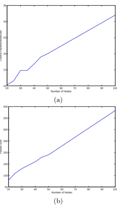
The amount of control traffic and message size were measured as the network size increased. We performed a set of experiments, each one 5 minutes long, where we varied the number of nodes from 20 to 50 (in increments of 5) and then 100. Figure 4 shows the effect of increasing the number of nodes in the topology to the number of control packets conveyed in the network and their size for a (Hello P eriod, RC P eriod) pair of (2,5) seconds.
Both the number and the size of packets vary linearly with the number of nodes. While the number of control messages can be reduced provided the accu-racy of monitoring is lowered, the RC message size depends on the routing table size of the nodes; with a pro-active routing protocol, each node holds entries for all nodes. Therefore, RC messages, even though optimized to include a node only once (see section 4) still holds at least all backbone nodes’ identities.
7
Conclusions and Future Work
In this article we have proposed a novel flow monitoring system for Wireless Mesh Networks with the goal of counting all of the flows passing through the backbone on only one mesh node, aiming to reduce export overhead. We build a monitoring overlay, in which a probe is able to decide if it monitors a flow that passes through its interfaces. We have described a protocol for probe organization that aims to reach the proposed goal. The protocol is based on a simple and minimal overhead routing table information flooding by all the probes. By sharing a global routing table view, the probes can trace the paths of the flows within the backbone, and therefore know what other nodes compete for monitoring the flows it sees. The metrics that make the difference in the decision process are chosen to minimize the flow record export: the distance from the collector, the connectivity degree and the up link quality.
We have evaluated the monitoring system to see its accuracy and the impact of the introduced management overhead. We determined the values of the inter-vals for sending control messages (Hello and RC messages) for a random number of topologies with 20 and 50 nodes, that optimize the number of management packets while keeping the accuracy of the monitoring system within acceptable limits.
In the future we plan to implement the proposed monitoring system on a small scale 802.11 mesh testbed, that we have set up in the lab. Secondly, since the monitoring system is based on the metrics advertised by the participating
20 30 40 50 60 70 80 90 100 10 15 20 25 30 35 Number of Nodes Control Packets/Node/Sec (a) 20 30 40 50 60 70 80 90 100 50 100 150 200 250 300 350 400 Number of Nodes Packet Size (b)
Fig. 4: (a) the average number of control packets per node per second as node size increases; (b) the average packet size as node size increases;
nodes, we investigate the situation where one or more nodes maliciously send faulty metrics, to either avoid monitoring (to save processing and communication bandwidth) or to monitor all traffic flows with the intention of eavesdropping, for instance. Another track of action is to find means to dynamically compute the values of the control message intervals, to adapt to the topology dynamics of the network. Recommended values (like the ones computed by us) are too general to fit the specificity of a community wireless mesh network (which depends a lot on conditions like geography or sources of interference).
Acknowledgement
This paper was partially supported by the French Ministry of Research project, AIRNET, under contract ANR-05-RNRT-012-01.
References
1. MIT Roofnet - 802.11b mesh network implementation. http://pdos.csail.mit.edu/roofnet/doku.php?id=design.
2. The Network Simulator NS-2 - http://www.isi.edu/nsnam/ns/.
3. UM-OLSR patch for ns-2 - http://masimum.dif.um.es/?Software:UM-OLSR. 4. Ian F. Akyildiz, Xudong Wang, and Weilin Wang. Wireless mesh networks: a
survey. Computer Networks, 47(4):445–487, March 2005.
5. Yigal Bejerano and Rajeev Rastogi. Robust Monitoring of Link Delays and Faults in IP Networks. In INFOCOM, 2003.
6. C. Chaudet, E. Fleury, I. Gu´erin-Lassous, H. Rivano, and M-E. Voge. Optimal po-sitioning of active and passive monitoring devices. In CoNEXT, Toulouse, France, October 2005.
7. T. Clausen and P. Jacquet. Optimized Link State Routing Protocol (OLSR). RFC Experimental 3626, Internet Engineering Task Force, Oct 2003.
8. Feiyi Huang, Yang Yang, and Liwen He. A flow-based network monitoring frame-work for wireless mesh netframe-works. Wireless Communications, IEEE, 14(5):48–55, October 2007.
9. Jun, Jangeun and Sichitiu, M. L. . The nominal capacity of wireless mesh networks.
Wireless Communications, IEEE, 10(5):8–14, 2003.
10. Kyu-Han Kim and Kang G. Shin. On accurate measurement of link quality in multi-hop wireless mesh networks. In MobiCom ’06, pages 38–49, New York, NY, USA, 2006. ACM Press.
11. John T. Moy. OSPF Version 2. Request for Comments 2328, Internet Engineering Task Force, April 1998.
12. Maitreya Natu and Adarshpal S. Sethi. Probe station placement for robust moni-toring of networks. J. Netw. Syst. Manage., 16(4):351–374, 2008.
13. Charles Perkins and Pravin Bhagwat. Highly Dynamic Destination-Sequenced Distance-Vector Routing (DSDV) for Mobile Computers. In ACM SIGCOMM’94, pages 234–244, 1994.
14. Alberto Gonzalez Prieto and Rolf Stadler. A-GAP: An adaptive protocol for contin-uous network monitoring with accuracy objectives. IEEE Transactions on Network
and Service Management (IEEE TNSM), 4(5), june 2007.
15. Francoise Sailhan, Liam Fallon, Karl Quinn, Paddy Farrell, Sandra Collins, Daryl Parker, Samir Ghamri-Doudane, and Yangcheng Huang. Wireless mesh network monitoring: Design, implementation and experiments. Globecom Workshops, 2007
IEEE, pages 1–6, Nov. 2007.
16. K. Suh, Y. Guo, J. Kurose, and D. Towsley. Locating network monitors: Complex-ity, heuristics and coverage. In Proceedings of IEEE Infocom, March 2005.