HAL Id: hal-03118389
https://hal.archives-ouvertes.fr/hal-03118389
Submitted on 22 Jan 2021HAL is a multi-disciplinary open access
archive for the deposit and dissemination of sci-entific research documents, whether they are pub-lished or not. The documents may come from teaching and research institutions in France or
L’archive ouverte pluridisciplinaire HAL, est destinée au dépôt et à la diffusion de documents scientifiques de niveau recherche, publiés ou non, émanant des établissements d’enseignement et de recherche français ou étrangers, des laboratoires
Monitoring discharge in a tidal river using water level
observations: Application to the Saigon River, Vietnam
B. Camenen, N. Gratiot, J.-A. Cohard, F. Gard, V.Q. Tran, A.-T. Nguyen, G.
Dramais, T. van Emmerik, J. Némery
To cite this version:
B. Camenen, N. Gratiot, J.-A. Cohard, F. Gard, V.Q. Tran, et al.. Monitoring discharge in a tidal river using water level observations: Application to the Saigon River, Vietnam. Science of the Total Environment, Elsevier, 2021, 761, pp.143195. �10.1016/j.scitotenv.2020.143195�. �hal-03118389�
Monitoring discharge in a tidal river using water level
observations: application to the Saigon River, Vietnam
B. Camenena,∗, N. Gratiotb,c, J.-A. Cohardb, F. Gardb, V. Q. Tranb,c, A.-T. Nguyenb,c, G. Dramaisa, T. van Emmerikd, J. N´emeryb,c
aInrae, UR RiverLy, centre de Lyon-Grenoble, Villeurbanne, France bCARE, IRD, Ho-Chi-Minh-City, Vietnam
cIGE, Univ. Grenoble Alpes / CNRS / IRD / Grenoble INP, Grenoble, France dHQWM, Univ. Wageningen, Wageningen, The Netherlands
Abstract
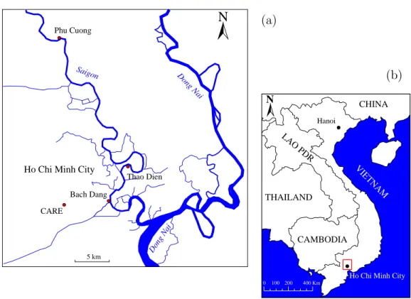
The hydrological dynamics of the Saigon River is ruled by a complex combination of factors, which need to be disentangled to prevent and limit risks of flooding and salt intrusion. In particular, the Saigon water discharge is highly influenced by tidal cycles with a relatively low net discharge. This study proposes a low-cost technique to estimate river discharge at high fre-quency (every 10 minutes in this study). It is based on a stage-fall-discharge (SFD) rating curve adapted from the general Manning Strickler law, and cal-ibrated thanks to two ADCP campaigns. Two pressure sensors were placed at different locations of the river in September 2016: one at the centre of Ho Chi Minh City and one in Phu Cuong, 40 km upstream approximately. The instantaneous water discharge data were used to evaluate the net resid-ual discharge and to highlight seasonal and inter-annresid-ual trends. Both water
level and water discharge show a seasonal behaviour. Rainfall, including during the Usagi typhoon that hit the megalopolis in November 2018, has no clear and direct impact on water level and water discharge due to the delta flat morphology and complex response between main channel and side channel network and ground water in this estuarine system under tidal in-fluence. However, we found some evidences of interactions between precip-itation, groundwater, the river network and possibly coastal waters. This paper can be seen as a proof of concept to (1) present a low-cost discharge method that can be applied to other tidal rivers, and (2) demonstrate how the high-frequency discharge data obtained with this method can be used to evaluate discharge dynamics in tidal river systems.
Keywords: Saigon River, water level, water discharge, tidal river, flood, stage-fall-discharge rating curve.
1. Introduction 1
A good understanding of the hydrological cycle, and discharge in partic-2
ular, in tidal rivers enables reliable forecasting and decision making by re-3
searchers and policy makers. Some priorities are generally put on the protec-4
tions against floods, saline intrusion and the dynamics of pollutants because 5
of the social, economic and political stakes they are linked to. Hydrological 6
cycles in Low Elevation Coastal (and deltaic) Zone (LECZ, 0-10 masl) differ 7
a lot from their upstream environments due to the tidal influence (van Driel
8
et al., 2015). Although this is a strategic zone at the interface between land 9
and ocean, physical and environmental data collected in this environment re-10
main sparse because of inherent logistical difficulties due to the unsteadiness 11
of the flow (Taniguchi et al., 2013). On one hand, the river water discharge 12
is influenced by tidal dynamics, which modulate hydrodynamics at high and 13
low frequency and can reshape the geomorphology, with feedback loops on 14
hydrodynamics (Mao et al., 2004). On the other hand, estuarine and deltaic 15
zones are highly influenced by peak fresh water discharges, which are them-16
selves modulated by tidal asymmetry (Sassi and Hoitink, 2013). 17
In the floodplain of the Saigon River, which is part of the LECZ of the 18
south of Vietnam, vulnerability could be assessed according to four factors 19
(McGranahan et al.,2007;van Driel et al.,2015) : (i) Relative Sea Level Rise 20
(RSLR) due to climate change and natural and anthropogenic subsidence; 21
(ii) Wetland ecological threat; (iii) Population pressure: and (iv) Delta gov-22
ernance (adaptivity, participation, fragmentation). The Saigon River flows 23
through Ho Chi Minh City (HCMC), a highly populated area, where popu-24
lation density can reach up to 30,000 inhabitants/km2 (Nguyen et al.,2019). 25
The unprecedented growth of HCMC induces pressure on the environment 26
and especially water resources (Van Leeuwen et al.,2016). 27
A major issue in such regions is to measure the instantaneous discharge 28
for a tidal river and to evaluate the residual discharge of the tide-affected 29
river. Indeed, a simple stage-discharge relationship cannot be used because 30
of the downstream influence of the tide. Stage-fall-discharge (SFD) rating 31
curves are traditionally and successfully used to compute discharge at sites 32
where variable backwater effects could affect a classical stage-discharge re-33
lationship (Rantz, 1982). Such methods have recently improved thanks to
34
Bayesian methods (Petersen-Øverleir and Reitan, 2009; Mansanarez et al., 35
2016). However, the relation between stage, slope, and discharge has
gen-36
erally been considered too complex in tidal rivers to attempt to obtaining 37
accurate discharges. Rantz (1963) proposed a graphical method using
mul-38
tiple correlation, which remains difficult to apply, especially when the tidal 39
influence leads to discharge fluctuations as large as the residual discharge. 40
That is the reason why there exists nearly no hydrometric stations world-41
wide in such rivers. Recently, acoustic sensing techniques (through HADCP, 42
Horizontal Acoustic Doppler Current Profiler) have been implemented suc-43
cessfully in some tidal rivers such as the Sacramento River, California (Ruhl
44
and DeRose, 2004) or in the rivers Berau and Mahakam in East Kaliman-45
tan, Indonesia (Hoitink et al., 2009; Sassi et al., 2011). Such techniques 46
generally correspond to a velocity index method. Similar method using an 47
ADP (Acoustic Doppler Profiler) current meter was deployed on the Tan-48
shui River, Taiwan (Chen et al., 2012b) or fixed ADCPs (Acoustic Doppler
Current Profiler) on the Yangtze River at Xuliujing, China (Zhao et al., 50
2016; Mei et al., 2019). These methods remain however expensive (around 51
30keexcluding structural works and maintenance) and difficult to display in 52
an urban place due to risk of vandalism. 53
In a recent work, Camenen et al. (2017) proposed to apply a stage-fall-54
discharge rating curve to estimate instantaneous discharges in tidal rivers. 55
Such simple model can be calibrated using intense discharge campaigns achieved 56
over a full tide cycle, which are easily available nowadays thanks to the ADCP 57
technology. The first application of the method was based on field measure-58
ments made on the Saigon River in September 2016 and was particularly 59
successful (Camenen et al., 2017). It presented some limitations for a very 60
asymetric tidal wave (close to a tidal bore), which is not the case for the 61
Saigon River. 62
In this paper, this simple low-cost water level-based discharge monitoring 63
is applied the Saigon River for a two-year period. A calibration and validation 64
of the method are first presented. The monitoring of two hydrological seasons 65
from January 2017 to Dec 2019 is then discussed. Results obtained allow for 66
examining and discussing two specific aspects : first, what is the hydrological 67
pattern of the Saigon River at different time scales, from the event scale to 68
years, and how is it influenced by the sea level ; second, how much the rainfall 69
regime is directly influencing the Saigon River dynamics, in particular, how 70
does the river react to extreme events? 71
2. Material and methods 72
2.1. Study site 73
The Saigon River is located in the South of Vietnam, in a low elevation 74
coastal zone, i.e. between 0 and 10 m above mean sea level (MSL, Figure 75
1). The Saigon River takes its source in Cambodia and is 225 km long.
76
Its catchment area has a surface of 4717 km2 (Nguyen et al., 2019). The
77
Saigon River is actually a complex river system, subject to several human 78
and environmental interactions, including many canals while it crosses Ho 79
Chi Minh City (HCMC) megalopolis, before flowing into the Dong Nai River 80
and the coastal waters. Upstream the megalopolis, the river is regulated by 81
the Dau Tieng dam, which was built during the 1980’s, in order to mitigate 82
saline intrusion and secure the fresh water supply uptake station of HCMC. 83
The situation of HCMC is all the more critical as 65% of the city is located 84
at an altitude of 1.5 m above MSL (Scussolini et al., 2017; Vachaud et al., 85
2019). 86
The flow of the Saigon River is predominantly driven by tidal currents, 87
which affects both the water level and water discharge, with regular exfil-88
tration of water in some urban districts during high spring tides. Over the 89
year, precipitation follow two contrasted seasons: the dry season, usually ex-90
N
Dong Nai Saigon Phu Cuong Dong Nai 5 km Thao Dien Bach DangHo Chi Minh City
CARE (a) (b) N 0 100 200 400 Km CAMBODIA Hanoi LAO PDR VIETNAM
Ho Chi Minh City THAILAND
CHINA
Figure 1: Location of the study site: the low elevation coastal zone of the Saigon River system, including the Saigon and Dong Nai rivers and Ho Chi Minh City (red points correspond to the position of pressure gauges).
tending from November to April and the wet season from May to October, 91
which gathers about 80% of the total rain (Nguyen et al.,2019). Rain event 92
can be severe and precipitation record can locally exceed 300 mm/day, even 93
400 mm/day. In this paper, we focus on one of the most severe rainy events 94
that experienced the city. It occurred in November 2018, when Usagi typhoon 95
hit HCMC. During this event, there was an increase of more than 300 mm 96
in rainfall which caused flooding, material and human damages reported in 97
several newspapers. 98
2.2. Water discharge estimation 99
The instantaneous water discharge was estimated by applying a stage-fall-100
discharge (SFD) rating curve adapted from the general Manning-Strickler 101
law, previously tested and validated by Camenen et al. (2017). This model
102
is based on the assumption of a pseudo-uniform flow and a prismatic sec-103
tion, which is valid for a low slope river with slowly varying water depth. 104
Considering an almost constant flow between two water level measures, the 105
Manning-Strickler equation can be applied : 106 Q = KAwR 2/3 h √ S (1)
with Q the water discharge [m3/s], K the Manning-Strickler coefficient [m1/3/s], 107
Rh = Aw/Pw the hydraulic radius [m], Aw the wet section [m2], Pw the wet 108
perimeter [m], and S the energy slope [-] assumed equal to the water slope. 109
Another assumption made here is that the river section and reach are stable 110
with no significant bed changes. It was verified by comparing the different 111
bathymetries from both ADCP campaigns. 112
Two hydrological stations are needed to evaluate the hydraulic slope of 113
the river: the water level zupand zdn were measured at Phu Cuong (upstream 114
station) and Bach Dang then Thao Dien stations (downstream stations), 115
which are named “PC”, “BD”, and “TD” hereafter (see Fig. 1a). Distance
between stations is around L = 42 km (PC-BD) and L = 35 km (PC-TD), 117
which is sufficient to have a significant difference in altitude and to estimate 118
slope with a good resolution for this low slope system. Due to tides and 119
flow oscillation, the slope oscillates between positive and negative values. 120
Also, the slope in Equation (1) (S = (zup− zdn)/L) does not correspond to 121
the local slope at the point in which the discharge is evaluated, i.e. at Phu 122
Cuong (PC). Indeed, because of the distance between the two stations, the 123
flow discharge is slightly different at the two stations. However, this spatial 124
offset can be translated as a lag time ∆t. As a consequence, the discharge 125
estimation at PC can be written : 126
Q(t) = KAw(zup(t))Rh(zup(t))2/3 q
|S(t + ∆t)| S(t + ∆t)
|S(t + ∆t)| (2)
By specifying the river cross-section at PC (assuming it is relevant for the 127
whole reach), one can easily evaluate Aw and Rh as a function of the water 128
level zup. In Equation (2), two parameters need to be calibrated : 129
- K, the Strickler coefficient of the river reach supposed homogeneous 130
between PC and BD, 131
- ∆t, a priori negative since the tide progresses from downstream to 132
upstream. 133
The Strickler coefficient could vary depending on the discharge due to addi-134
tional head losses at low flows (emergence of sills) or at high flows (flood-plain 135
interaction). Nevertheless, such cases were not observed for the specific case 136
of the Saigon River. 137
2.3. Water level measurement 138
To apply Equation (2), CTD Diver sensors were installed at PC and BD
139
stations in September 2016, as reported in Figure 1. They measure pressure, 140
conductivity and temperature every 10 minutes. Conductivity and temper-141
ature were considered as interesting proxy to interpret data series and were 142
used to operate the post processing, but were not used directly in this study. 143
PC sensor was immersed in the river bank of the Saigon River, close to Phu 144
Cuong city, TD sensor was immersed in the heart of the megalopolis of Ho 145
Chi Minh City, in Thao Dien district. Both sensors were downloaded at a 146
bimonthly basis. Due to logistical constraints, significant risks of theft and 147
of mechanical deterioration, TD station was displaced twice with a corre-148
sponding adjustment of parameters in Equation (2) (L and ∆t). The sensor
149
was initially installed in Bach Dang, in the city centre in September 2016. It 150
was moved to Boat House (BH), 8.5 km upstream of the Bach Dang point, 151
from January 2017 to the 8th of March 2017. Then, since 15th March 2017, 152
the sensor is located in Thao Dien Village (TD). Distance between those 153
two last sites is only 0.9 km. To compensate water level measurements from 154
atmospheric pressure fluctuations, a barometer was installed at the CARE 155
center (Ho Chi Minh University of Technology, see Figure 1). 156
Some drifts of the water level measurements were observed due to fine 157
deposit accumulation leading to over-pressure. Water levels at PC and TD 158
were thus corrected based on monthly campaigns made by Sub Institute 159
of Hydrometeorology and Climate Change (SIHYMECC, also named CEM 160
hereafter for Center of Environmental Monitoring) of Ho Chi Minh City. 161
During these campaigns, water levels were measured every hour for three 162
days at the staff gauge. In Figure 2, one can observed a very good agreement 163
between CTD Diver data and SIHYMECC data (the water level H cor-164
responds the the difference between the water surface level and a reference 165
level of the station). 166 (a) (b) 24/06/17 25/06/17 26/06/17 27/06/17 -2 -1 0 1 2 H [m] 24/06/17 25/06/17 26/06/17 27/06/17 -2 -1 0 1 2 H [m]
Figure 2: Comparison between water levels H measured at PC (a) and TD (b) stations and water levels measured by the SIHYMECC at the staff gauges for the selected period between 24th to 27th of June 2017.
2.4. Residual discharge 167
In order to study the net water discharge in the Saigon River and eval-168
uate the hydrological cycle, the instantaneous water discharge needs to be 169
averaged over four tide periods (Ttide = 12.4 hours) to filter the 1st order 170
semi-diurnal tidal signal from the data-series. As a consequence, Qn(t0) = 171
Rt0+2Ttide
t0−2Ttide Q(t)dt. In the same way, the tidal averaged water level can be ob-172
tained such as zta(t0) =
Rt0+2Ttide
t0−2Ttide z(t)dt. The acquisition of data at high 173
frequency (every 10 minutes) and over a longer period (two hydrological sea-174
sons) is a prerequisite to such evaluation. 175
3. Calibration and validation of the SFD rating curve 176
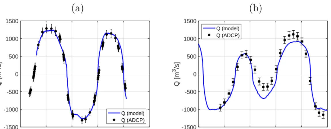
3.1. Calibration of the model using ADCP campaigns 177
Two Acoustic Doppler Current Profiler (ADCP) campaigns have been led 178
in September 2016 and March 2017 with a Rio Grande 600 kHz (Dinehart
179
and Burau, 2005). During 24 hours and for every hour, one gauging, i.e. 180
three transects, was realized at PC with a boat and a georeferenced ADCP 181
mounted on it. ADCP campaigns were used to calibrate the water discharge 182
estimation, calculated with Equation (2) (Camenen et al., 2017). K and
183
∆t were calibrated such as the modelled discharge fit to observed data (see 184
also appendix Appendix A.1). Also, since it is very difficult to evaluate the 185
exact vertical reference level of each station, these campaigns were used to 186
optimize the measured difference zup− zdn using an additional parameter ∆z 187
(i.e. zup− zdn = (zup− zdn)measured+ ∆z) 188
To ensure the robustness of the hydraulic model, calibration were real-189
ized during both wet (September 2016) and dry (March 2017) seasons. These 190
ADCP campaigns were also used to determine the river cross-section char-191
acteristics, to calculate Aw and Rh as a function of water level. Error in 192
ADCP measurements were evaluated at 10% using a minimum error value of 193
100 m3/s since the conditions were adverse (Le Coz et al., 2016). We found 194
the best results using a Manning-Strickler coefficient K = 26 m1/3/s and
195
∆t = −2.0 hours (see Appendix Appendix A.1). Results are presented in
196
Fig. 3. Very good results can be observed for the September 2016 campaign.
197
Some slight error may be observed at the end of the first flow peak (Fig. 198
3a, at around 21 h, local time) but it is due to a pressure gauge outside
199
water. For the 2017 campaign, results are not as accurate but still in good 200
agreement with data. The clear asymmetric semi-diurnal tidal signal for this 201
specific day may explain some of the differences (Camenen et al., 2017). 202
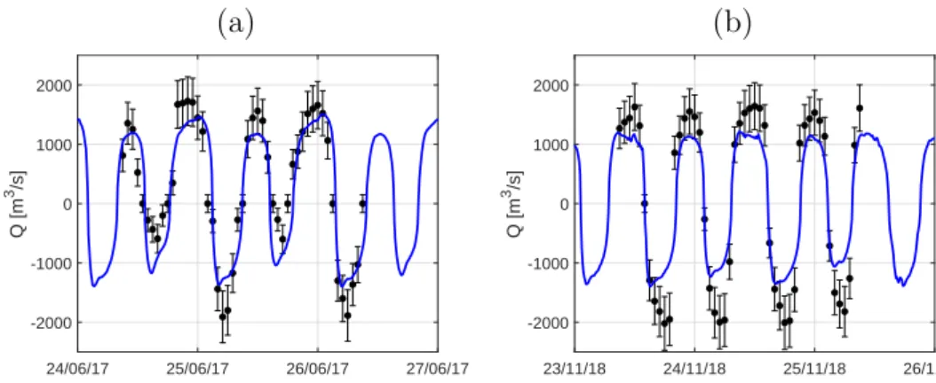
3.2. Validation of the model using other discharge estimations 203
The monthly campaigns made by SIHYMECC also include some dis-204
charge estimation every hour for 48 h. They applied the velocity index
205
method by measuring the water level and the depth-averaged velocity uindex
(a) (b) 13/09:12h13/09:18h 14/09:0h 14/09:6h 14/09:12h14/09:18h -1500 -1000 -500 0 500 1000 1500 Q [m 3/s] Q (model) Q (ADCP) 21/03:6h 21/03:12h21/03:18h 22/03:0h 22/03:6h 22/03:12h -1500 -1000 -500 0 500 1000 1500 Q [m 3 /s] Q (model) Q (ADCP)
Figure 3: Water discharge Q comparison between model results and ADCP mea-surement campaigns in September 2016 (a) and March 2017 (b).
at one location yindex (Chen et al., 2012b) : 207
Q = αindexuindexAw (3)
with αindex= 0.8 a calibration coefficient, αindex= U/uindexwhere U = Q/Aw 208
the section-averaged velocity. Again, since conditions are adverse, we roughly 209
estimated the error from this method equal to 15% plus a minimum error of 210
150 m3/s based on Ruhl and Simpson (2006). 211
The corresponding water discharge estimated from Equation (2) are in
212
good agreement with data from SIHYMECC (Fig. 4). The model tends to
213
yield smaller peak values for the inward discharge (negative), even if this 214
trend is not observed for all tidal cycles. This tendency is more pronounced 215
for the 2018 data (Fig. 4b). This could be the consequence of either a
216
varying flow repartition throughout the river section during the ebb and flow 217
not caught by the index velocity method or a bias on the slope estimation 218
by the proposed model based on a slope downstream of the station. 219 (a) (b) 24/06/17 25/06/17 26/06/17 27/06/17 -2000 -1000 0 1000 2000 Q [m 3 /s] 23/11/18 24/11/18 25/11/18 26/11/18 -2000 -1000 0 1000 2000 Q [m 3/s]
Figure 4: Water discharge Q estimated at PC (blue line) in comparison to SI-HYMECC data for two contrasting hydrological periods in June 2017 (a) and in November 2018 (b).
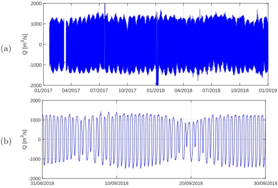
4. A two-year monitoring of the Saigon River 220
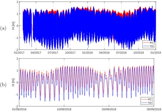
4.1. Water levels 221
The water level time series, which covers two hydrological years, from 222
January 2017 to December 2018 are reported in Figure5a. For both stations, 223
the reference level is the one of the staff gauge, which explains the existence 224
of some negative values. 225
In each panel, one can see that the tidal signal clearly predominates with 226
a strong semi-diurnal harmonic. The cyclicity is particularly emphasized 227
through the examination of a zoomed period in September 2018 (Figure 228
(a) 01/2017 04/2017 07/2017 10/2017 01/2018 04/2018 07/2018 10/2018 01/2019 -2 -1 0 1 2 H [m] PC TD (b) 31/08/2018 10/09/2018 20/09/2018 30/09/2018 -2 -1 0 1 2 H [m] PC TD
Figure 5: Two-year water level time series measured at PC and TD (a) with a zoom in September 2018 (b).
5b). The cyclicity is evidenced on both PC and TD stations, who present
229
synchronous fluctuations, with a time laps of about 1 hour and 10 minutes, 230
which corresponds to the duration of tide wave propagation between the two 231
stations. The tidal magnitude is smaller at PC station (by 17%) than at TD 232
station, which is physically consistent with quadratic friction dissipation: the 233
further upstream the station is, the less it is influenced by tidal waves. Tidal 234
range was measured to oscillate between -2.00 m and 1.50 m at both TD and 235
PC stations. 236
A first glimpse of seasonality can be observed in the two-year time-series. 237
One can observe lower water levels in the rainy season (May to September) 238
and higher values in the dry season (November to March). Semi-diurnal tidal 239
forcing clearly prevails on the Saigon River. As illustrated in Figures2and5, 240
the 14-days cycle presented both symmetric and asymmetric tides; a pattern 241
which is particularly well developed in the estuaries located in the south of 242
Vietnam (Chen et al.,2012b). 243
4.2. Continuous discharge estimation 244
By applying Equation (2), one can easily calculate the discharge at PC 245
using water levels from both PC and TD stations. Water discharge is domi-246
nated by tidal semi-diurnal harmonics, as for water level data-series (Figure 247
6). Instantaneous discharge ranged from -2000 to 2000 m3/s. The
oscilla-248
tion of the magnitude of tides, between spring and neap tides, is also well-249
identified (Figure6b). Maxima appears at every syzygy between the sun, the 250
moon and the earth. Overall, the analysis of instantaneous water discharge 251
highlighted the predominant forcing of tides on any other forcing, despite 252
contrasted and well-marked dry and rainy seasons. 253
4.3. Residual discharge 254
All data from the SIHYMECC field campaigns (which correspond to a 255
48 h experiment ≈ 4Ttide) were compared to the proposed model (Figure7a). 256
As expected, since the model yields smaller amplitudes (see Figure 4), one
(a) 01/2017 04/2017 07/2017 10/2017 01/2018 04/2018 07/2018 10/2018 01/2019 -2000 -1000 0 1000 2000 Q [m 3 /s] (b) 31/08/2018 10/09/2018 20/09/2018 30/09/2018 -2000 -1000 0 1000 2000 Q [m 3/s]
Figure 6: Two-year water discharge time-series (a) with a zoom in September 2018 (b) at Phu Cuong (PC).
generally finds a good correlation but with few outliers, predominantly above 258
the 1:1 line for negative discharge and bellow the 1:1 line for positive discharge 259
(i.e. |Qmodel|lsim|Q(CEM )|). One should note also the many zero values for 260
the SIHYMECC (CEM) data, which may be the consequence of a human bias 261
(while reading the staff gauge) and partly explains uncertainties in experi-262
mental data and some of the scatter in the model response. A comparison of 263
the net water discharge measured by the SIHYMECC and modelled by our 264
group is reported in Figure 7b for the 18 SIHYMECC campaigns available.
265
One can realize the order of magnitude of difference between maximum in-266
stantaneous discharges and net discharges, which corresponds to the red box 267
in Figure 7a. Despite the existence of few outliers, modelled points for net 268
water discharge are well correlated with the estimation from measured data. 269
As expected, since the model yields smaller amplitudes, the net discharge 270
estimations are generally smaller. The existence of outliers is not surpris-271
ing looking at the sensitivity of such calculation while net discharge is one 272
order of magnitude smaller than peak values (positive and negative). But 273
surprisingly, while SIHYMECC estimations of the net discharge are always 274
positive, the proposed model leads sometimes to negative values. Although 275
difficult to explain, these negative values may results from a combination of 276
factors, such a the asymmetrical tides and complex exchanges with ground-277
water and with the canal network. The regular occurrence of salt intrusions 278
up to HCMC does confirm the possible occurrence of a net negative water 279
discharge. Also, as discussed above, the model is very sensitive to a possible 280
error in water level estimation a PC and BD, TD stations. Hence, for the 281
net discharge, we evaluated the error equal to 20 m3/s per cm of error in the 282
vertical axis (See Appendix Appendix A.3).
283
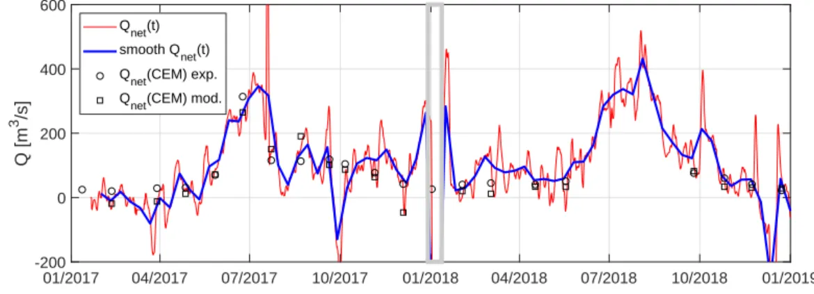
The net discharge time series over this two-year experiment is presented in 284
Figure 8. Compared to monthly SIHYMECC campaigns, we observe more
285
variability in the net discharge time-series. Some spikes are however not 286
realistic and result from data gaps (January 2018, December 2019). 287
(a) (b) -2000 -1000 0 1000 2000 Q (CEM) [m3/s] -2000 -1000 0 1000 2000 Q (model) [m 3/s] R2 = 0.91 0 50 100 150 Qnet (CEM) [m3/s] -50 0 50 100 150 Q net (model) [m 3/s] R2 = 0.55
Figure 7: Comparison of the instantaneous (a) and net (b) discharges obtained by the SIHYMECC (CEM) and the proposed model for all 2017 and 2018 SIHYMECC campaigns.
The seasonality of precipitation in this tropical humid low lying area 288
is expectedly a main driver of the annual hydrological cycle, but as shown 289
previously, this driver is masked by the tidal forcing (Figure 8). The wet
290
season is expectedly linked with a higher water discharge and a refill of 291
the groundwater. At the opposite, the dry season is expectedly linked with 292
a decrease of the net water discharge. This general pattern was broadly 293
described by Nguyen et al. (2019), but needs to be detailed and should be
294
understood on a physically based characterization of the main drivers. One 295
can clearly observe the seasonality of net discharge with peak values during 296
the wet season in Figure8. In 2017, the peak net discharge reached 300 m3/s 297
and lasted only for two months in the beginning of June and the end of 298
July. In 2018, net discharges exceeded 200 m3/s from June to August with 299
maximum values up to 400 m3/s. It then decreased before a second peak
300
was reached in early October. Flood extended for more than four months, 301
leading to one of the most humid year of the decade (Fig. 8 and Fig. 10). 302 01/2017 04/2017 07/2017 10/2017 01/2018 04/2018 07/2018 10/2018 01/2019 -200 0 200 400 600 Q [m 3 /s] Qnet(t) smooth Q net(t) Qnet(CEM) exp. Qnet(CEM) mod.
Figure 8: Net discharge Qnetestimate for the January 2017 - December 2019 period
(full lines correspond to the model results while symbols correspond to values for the SIHYMECC campaigns using their own estimations -exp.- or using the model -mod.-; the grey line delimits a period of missing data at PC).
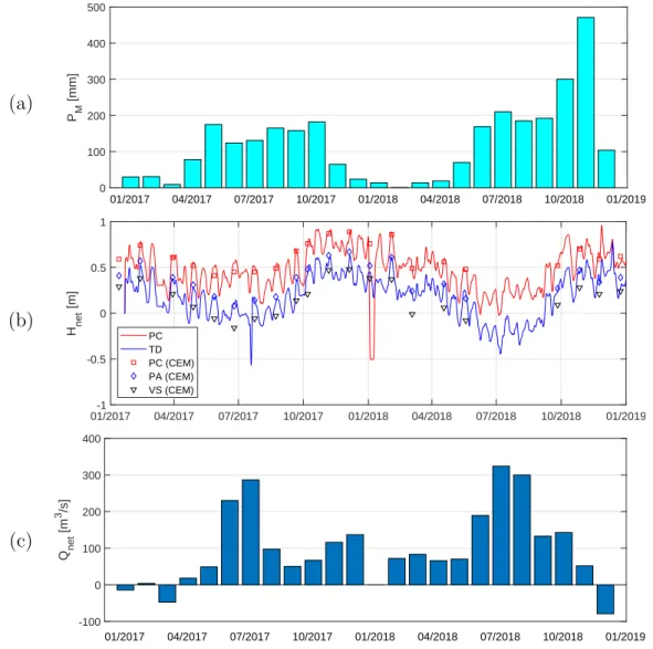
Monthly cumulated precipitation, tide-averaged water level along the 303
Saigon and Dong Nai rivers and monthly averaged net-discharge are pre-304
sented in Figure 9 for the 2017 and 2018 periods. 2017 and 2018 rainy
305
seasons are well-marked, with an increase in precipitation from June to Oc-306
tober. In 2018, precipitations are particularly high and extended in October 307
and November. The tide-averaged water level follows the rain pattern for 308
both increasing and decreasing phases, with a shift of two to three months. 309
Concerning the averaged water discharge, it was measured to fluctuate be-310
tween -100 to 500 m3/s (no value is given for January 2018 since there was a 311
too long gap in data), with a magnitude that was quite different for both hy-312
drological years. In 2017, one can noticed that there exists an expected time 313
lag between rain (first) and river discharge (few weeks later) but there is also 314
some delayed and complex interactions with groundwater and/or water level. 315
The rainy season, which started in May, was followed by a rise in the net 316
water discharge only one month later (June) and then, by an increase of the 317
tide-averaged water level few weeks later (July, August). Also, one observed 318
a drop in net discharge in August and September, while precipitation remains 319
high followed by a rise in net discharge while precipitation dropped. It seems 320
there are strong exchanges of water with groundwater and/or floodplain with 321
a possible recharge from the groundwater and/or floodplain in May, August 322
and September and a restitution to the river in November and December. 323
However, Van and Koontanakulvong (2018) estimated possible exchanges of
324
water between the aquifer and the Saigon River of approximately 0.02 m3/s
325
per km, which appears negligible. Effects of the large drainage and canal 326
system around the Saigon River (i.e. of the Saigon floodplain) may prevail 327
here. Also, anthropogenic influences such as Dau Tieng dam management 328
or water supply pumping may significantly affect the net Saigon river water 329
discharge. In 2018, cumulated rain also led to an increase of the net water 330
discharge, but the rise of the Saigon River discharge was much faster and 331
almost correlated to precipitation, which lets presume that soil saturation 332
was higher and led to a direct response of the river to precipitation. Even 333
if rain initiated late in the season, as compared with year 2017 (May and 334
June in 2018 instead of April and May in 2017), the shape and cumulative 335
rain during the rainy season was quite comparable to 2017. The net water 336
discharge responded similarly to 2017 in June 2018. However, in 2018 the 337
response to precipitation is stronger with a monthly averaged net discharge 338
above 400 m3/s in July and August. Surprisingly, in October and November,
339
while precipitation is particularly high in fall and superimposed with the ex-340
treme typhoon event in late November, one can observe a decrease of the net 341
discharge. Significant floods have been observed during this period; a large 342
part of the water volume from precipitation may have been spread over the 343
flood plain. 344
Looking at the tide-averaged water level (Figure 9b) measured at Phu
345
Cuong (PC), Thao Dien (TD) or Phu An (PA), but also at Vam Sat (station 346
located downstream on the Dong Nai River at approximately 20 km from the 347
see shore), a clear annual fluctuation can be observed with high water levels 348
from October to April. Such high values yield an averaged negative slope 349
leading some counter-effects on the net discharge (see Appendix Appendix
350
A.3). Interestingly, these fluctuations are not correlated to precipitations 351
and could partially explain the deficit in net water discharge compared to 352
precipitation. We suspect these fluctuations to be a consequence of the peak 353
flow season of the Mekong River, which occurs in October in coastal flood-354
plain and could influence sea water levels next to its river mouth (Chen et al., 355
2012a; Ho et al.,2014;Thi Ha et al., 2018). 356 (a) 01/2017 04/2017 07/2017 10/2017 01/2018 04/2018 07/2018 10/2018 01/2019 0 100 200 300 400 500 PM [mm] (b) 01/2017 04/2017 07/2017 10/2017 01/2018 04/2018 07/2018 10/2018 01/2019 -1 -0.5 0 0.5 1 H net [m] PC TD PC (CEM) PA (CEM) VS (CEM) (c) 01/2017 04/2017 07/2017 10/2017 01/2018 04/2018 07/2018 10/2018 01/2019 -100 0 100 200 300 400 Q net [m 3/s]
Figure 9: Monthly rainfall PM (a), tide-averaged water levels Hnet(b) and monthly
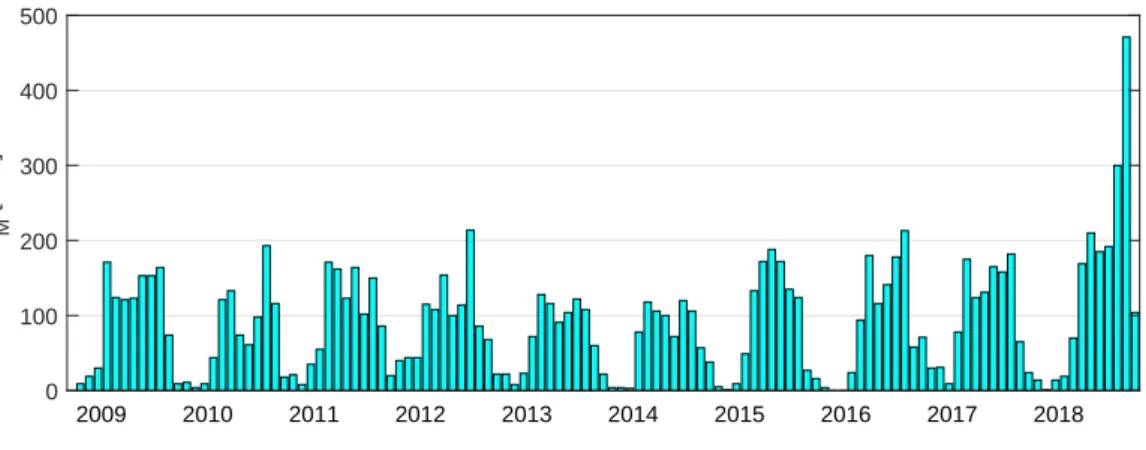
4.4. Effects of long-term precipitation 357
To get further in the analysis of the interaction between the Saigon River 358
discharge and its surrounding floodplain, we examined a pluriannual monthly 359
rainfall series (Figure 10). This series was associated with the severe Ni˜no 360
event in 2015-2016 (Thirumalai et al., 2017; Thi Ha et al., 2018). In Figure 361
10, one can observed a regular decrease of annual precipitation from 2009
362
to 2012, a minimum from 2013 to 2015 and an increase until 2019. The 363
2013-2015 period thus corresponded to a deficit of rain, which was evidenced 364
by socio-political impacts described in newspapers, particularly during the 365
dry season 2015-2016. This dry season was reported as the worst drought 366
ever reported in 98 years of monitoring in the floodplains of Mekong and 367
Saigon-Dong Nai hydrosystems. 368 2009 2010 2011 2012 2013 2014 2015 2016 2017 2018 0 100 200 300 400 500 P M [mm]
Figure 10: Monthly rainfall PM at HCMC from 2009 to 2019.
The 2017-2018 and 2018-2019 hydrological seasons that are reported in 369
Figure9support the hypothesis of a phase of recovery after these pluri-annual 370
droughts. The 2017 wet season showed a priori an atypical hydrological 371
response, with a normal rainy season from May to October, that is not in 372
correlation with water discharge due to strong exchanges with groundwater. 373
There is indeed a shift between the discharge increase and the precipitation 374
increase. This may result of years of deficit in the groundwater. 375
In 2018, the precipitation-river interaction was noticeably different. It 376
seems the groundwater recovered from the drought leading to a more typical 377
response of the river to precipitation. We may hypothesize that regional 378
recovery of rain during the last wet seasons (2016-2018) led to a recharge 379
of the groundwater table, and further of the river, presumably because the 380
floodplain had fully recovered from the pluri-annual drought that hit the 381
region from 2013 to 2016. 382
4.5. Effects of an extreme event : the Usagi typhoon 383
On November 25th 2018, HCMC was hit by Usagi typhoon. Arriving from 384
the East-south east, it reached the coast, at 50 km of Ho Chi Minh City (Ba 385
Ria-Vung Tau Province) in the morning. It continued moving Northwest 386
ward inland over HCMC area as a tropical depression. According to the 387
forecast department of the Southern Centre for Hydro-Meteorological Fore-388
casting (SCHMF), this was the highest ever recorded rainfall in a 24-hours 389
period in the megalopolis. Districts of HCMC recorder cumulated daily rain 390
between 293 to 408 mm for independent stations of measurements. While 391
there is no debate concerning the intensity of Usagi event and the severity 392
of damages, there is a clear interest in understanding how the hydrosystem 393
physically behaved during and just after those exceptional rains. The para-394
doxical result is the lack of direct response of the Saigon River to the extreme 395
precipitations. As shown in Figure 5, none of the two hydrological stations 396
recorded any consistent rise of the water level during the typhoon, neither 397
any flash rise of the river discharge (Figure 6). The only noticeable impact 398
recorded by our CTD sensors was a slight reduction of the conductivity at 399
the PC station, which dropped of a few percent when Usagi typhoon hit the 400
region (not shown in this paper). Could we conclude that the typhoon had 401
no effects on the river dynamics? Has the Dau Tieng dam totally regulated 402
the flow? 403
By comparing data from November 2017 and November 2018, one can 404
observe that despite a rise of rainfall by a factor six, mean water level and net 405
discharge reduced during this period by 15% (0.77 m in Nov. 2017 and 0.66 m 406
in Nov. 2018) and 50% (65 m3/s in Nov. 2017 and 30 m3/s in Nov. 2018),
407
respectively. It clearly shows that floods observed in some districts of the 408
city during the event were not directly driven by the overflow of water from 409
the river, but certainly by intense run off over impervious streets (Figure ??). 410
Also, we should not underestimate the potential impact of the Dau Tieng 411
dam management; large amount of water may have been retained during the 412
flood and slowly reinjected in the river during the following weeks. Finally, 413
since tide-average water levels in the Saigon River are relatively higher in 414
late fall (Fig. 9), and because of the storm surge, evacuation of water may 415
have been more difficult. This can be explained by the morphology of the 416
delta, which is very flat and close to the sea shore. Results from Scussolini
417
et al. (2017) showed the influence of the sea level on HCMC flood risk. Ho
418
et al. (2014) argued that main hydrological explanations for the flood risk 419
on HCMC area are the upstream floods including those of the Dong Nai and 420
Mekong delta, local rainfall, land subsidence, and sea level rise. Our results 421
indicate that local rainfall and sea water level may be the most impacting 422
factors. 423
5. Conclusion 424
Tidal rivers and their floodplains are environments that are hardly moni-425
tored although they concentrate most of the human activities and form habi-426
tats for rich ecosystems. Flood risk is a particular issue for such environment 427
and requires a good monitoring and a good understanding of its hydrological 428
functioning. 429
Here, we applied a stage-fall-discharge rating curve adapted from the gen-430
eral Manning-Strickler law (Camenen et al.,2017) to assess the instantaneous 431
water discharge on the Saigon River. For the first time, the Saigon River dy-432
namics was recorded at high frequency over two hydrological years, including 433
the heaviest rain event ever recorded. Such tool appears to be a very effi-434
cient and low cost system for estimating discharge in tidal rivers as soon as 435
the tidal wave is not too asymmetric and the river bed is stable (no general 436
erosion nor aggradation). One issue remains the estimation of the slope since 437
the model is sensitive to possible errors in water level measurements. This is 438
particularly true for the Saigon River, which is tide dominated. 439
The analysis of the data-series highlights the driving role of tides on water 440
mixing and water dynamics at hourly to monthly timescales. Once filtered 441
from tidal effects, the averaged water level and water discharge points out a 442
rather small contribution of run-off and a potential significant impact of flood 443
plain and anthopogenic structures (Dau Tieng dam, canals, water pumping, 444
etc.) to the hydrosystem response. The study of river response during Usagi 445
typhoon illustrated how much the floodplain can attenuate the direct impact 446
of intense precipitations and how critical is the sea water level to evacuate 447
the flood. Also, the seasonal variability of the tidal-averaged water levels 448
showed a possible influence of the nearby Mekong high flows that reduces 449
the slope and limits the net discharge. 450
This study remains a preliminary study, which needs to be completed with 451
some further studies on groundwater and flood plain dynamics, including 452
the complex canal network in HCMC to get an accurate evaluation of the 453
vulnerability of the megalopolis to flooding during extreme events and how 454
this vulnerability will evolve during coming decades under a worrying context 455
of subsidence and sea level rise. 456
Acknowledgements 457
This study was supported by the Rhˆone-Alpes region through the CMIRA
458
Coopera financial support. We also wish to thank all the interns who worked 459
on that topic throughout the last two years : R´emi Saillard, Lucas Barbieux, 460
Roman Smoliakov and Swann Benaksas, as well as everyone involved in the 461
two 24 hours field campaigns, which made the calibration possible. We are 462
grateful to Dr. Nguyen Phuoc Dan from CARE center (HCMUT) and Dr 463
Nguyen Van Hong from the sub-institute of hydrometeorology and climate 464
change center (SIHYMECC) for providing us the field measurements of water 465
level and water discharges. 466
References
Camenen, B., Dramais, G., Le Coz, J., Ho, T.-D., Gratiot, N., and Piney, S. (2017). Estimation d’une courbe de tarage hauteur-d´enivel´ee-d´ebit pour une rivi`ere influenc´ee par la mar´ee. La Houille Blanche, 5:16–21. (in French).
Chen, C., Lai, Z., Beardsley, R. C., Xu, Q., Lin, H., and Viet, N. T. (2012a). Current separation and upwelling over the southeast shelf of Vietnam in the South China Sea. Journal of Geophysical Research, 117(C03033):1–16.
Chen, Y.-C., Yang, T.-M., Hsu, N.-S., and Kuo, T.-M. (2012b). Real-time discharge measurement in tidal streams by an index velocity. Environmen-tal Monitoring & Assessment, 184:6423–6436.
Dinehart, R. L. and Burau, J. R. (2005). Repeated surveys by acoustic Doppler current profiler for flow and sediment dynamics in a tidal river. Journal of Hydrology, 314(1-4):1–21.
Ho, L. P., Nguyen, T., Chau, N. X. Q., and Nguyen, K. D. (2014). Integrated urban flood risk management approach in contextof uncertainties: case study Ho Chi Minh city. La Houille Blanche, 6:26–33.
Hoitink, A. J. F., Buschman, F. A., and Vermeulen, B. (2009). Continu-ous measurements of discharge from a horizontal acContinu-oustic Doppler current profiler in a tidal river. Water Resources Research, 45(11 ( W1140)):1–13.
Le Coz, J., Blanquart, B., Pobanz, K., Dramais, G., Pierrefeu, G., Hauet, A., and Despax, A. (2016). Estimating the uncertainty of streamgauging techniques using in situ collaborative interlaboratory experiments. Journal of Hydraulic Engineering, 509:573–587.
Mansanarez, V., Le Coz, J., Renard, B., Lang, M., Pierrefeu, G., and Vauchel, P. (2016). Bayesian analysis of stage-fall-discharge rating curves and their uncertainties. Water Resources Research, 52:7424–7443.
Mao, Q., Shi, P., Yin, K., Gan, J., and Qi, Y. (2004). Tides and tidal currents in the Pearl River Estuary. Continental Shelf Res., 24(16):1797–1808.
McGranahan, G., Balk, D., and Anderson, B. (2007). The rising tide: As-sessing the risks of climate change and human settlements in low eleva-tioncoastal zones. Environment and Urbanization, 19(1):17–37.
Mei, X., Zhang, M., Dai, Z., Wei, W., and Li, W. (2019). Large addition of freshwater to the tidal reaches of the yangtze(changjiang) river. Estuaries & Coasts, 42:629–640.
Nguyen, T. T. N., N´emery, J., Gratiot, N., Strady, E., Tran, V. Q., Nguyen, A. T., Aim´e, J., and Peyne, A. (2019). Nutrient dynamics and eutrophica-tion assessment in the tropical riversystem of Saigon – Dongnai (southern Vietnam). Science Total Environment, 653:370–383.
Petersen-Øverleir, A. and Reitan, T. (2009). Bayesian analysis of stage-fall-discharge models for gauging stations affected by variable backwater. Hydrological Processes, 23(21):3057–3074.
Rantz, S. E. (1963). An empirical method of determining momentary dis-charge of tide-affected streams. Water-Supply Paper 1586-D, U. S. Geo-logical Survey, Washington, USA. 33 p.
Rantz, S. E. (1982). Measurement and computation of streamflow: Volume 2. Computation of discharge. Water-Supply Paper 2175, U. S. Geological Survey. 313 p.
Ruhl, C. A. and DeRose, J. B. (2004). Monitoring alternatives at the Sacra-mento River at Freeport, California: results ofthe 2002–2004 pilot study. Technical Report Scientific Investigation Report 2004–5172, U. S. Geolog-ical Survey, Reston, Virginia.
Ruhl, C. A. and Simpson, M. (2006). Computation of discharge using the index-streamflow: method in tidally affected areas. Technical Report Sci-entific Investigations Report 2005–5004, U. S. Geological Survey, Reston, Virginia.
Sassi, M. G. and Hoitink, A. J. F. (2013). River flow controls on tides
and tide-mean water level profiles in a tidal freshwater river. Journal of Geophysical Research, 118:4139–4151.
Sassi, M. G., Hoitink, A. J. F., Vermeulen, B., , and Hidayat (2011). Discharge estimation from H-ADCP measurements in a tidal river
sub-ject to sidewall effects and a mobile bed. Water Resources Research, 47(W06504):1–14.
Scussolini, P., Tran, T. T. V., Koks, E., Diaz-Loaiza, A., Ho, P. L., and Lasage, R. (2017). Adaptation to sea level rise: Amultidisciplinary analysis for ho chiminh city, vietnam. Water Resources Research, 53:10,841–10,857.
Taniguchi, M., Allen, D., and Gurdak, J. (2013). Optimizing the water-energy-food nexus in the Asia-Pacific Ring of Fire. Eos, Transactions of the American Geophysical Union, 94(47).
Thi Ha, D., Ouillon, S., and Van Vinh, G. (2018). Water and suspended sediment budgets in the Lower Mekong from high-frequency measurements (2009–2016). Water, 10(7, 846):1–24.
Thirumalai, K., DiNezio, P. N., Okumura, Y., and Deser, C. (2017). Extreme temperatures in Southeast Asia caused by El Ni˜no and worsened by global warming. Nature Communications, 8(15531).
Vachaud, G., Quertamp, F., Phan, T. S. H., Tran Ngoc, T. D., Nguyen, T., Luu, X. L., Nguyen, A. T., and Gratiot, N. (2019). Flood-related risks in ho chi minh city and ways of mitigation. Journal of Hydrology, 573:1021–1027.
Van, T. P. and Koontanakulvong, S. (2018). Groundwater and river interac-tion parameter estimainterac-tion in Saigon River, Vietnam. Engineering Journal, 22(1):257–267.
van Driel, W. F., van, Bucx, T., Makaske, A., van de Guchte, C., van der Sluis, T., Biemans, H., Ellen, G. J., van Gent, M., Prinsen, G., and Adri-aanse, B. (2015). Vulnerability assessment of deltas in transboundary river basins. techreport Report 9, Delta Alliance International, Wageningen-Delft, The Netherlands. Delta Alliance contribution to the Transboundary Water Assessment Program, River Basins Assessment.
Van Leeuwen, C. J., Dan, N. P., and Dieperink, C. (2016). The challenges of water governance in Ho Chi Minh City. Integrated Environmental As-sessment & Management, 12(2):345–352.
Zhao, J., Chen, Z., Zhang, H., and Wang, Z. (2016). Multiprofile discharge estimation in the tidal reach of Yangtze Estuary. Journal of Hydraulic Engineering, 142(12, 04016056):1–12.
Appendix A. Sensitivity analysis
Appendix A.1. Error calculation on experimental data
A first sensitivity analysis was made to optimize main model parameters (Strickler coefficient K and the time shift ∆t) to experimental data. For
both ADCP campaigns in September 2016 and March 2917 (see Figure 3),
the estimation of the error was made using the mean square error :
E(Q) = s
1 nΣ
n
i=1[Qmod.(ti) − Qmeas.(ti)]2 (A.1)
where n is the number of gauging data, Qmod. the modelled discharge and
Qmeas. the measured discharge, and ti the time of each of these gauging.
As can be observed in Fig. A.11, errors are significantly smaller for the
first campaign for which the tide was more symmetrical. Indeed, E(Q) ≈
200 m3/s for the September 2016 campaign whereas E(Q) ≈ 350 m3/s for
the March 2017 campaign. From this sensitivity analysis, one would choose
K = 25 m1/3/s and ∆t = −2.04 h. (a) (b) 18 20 22 24 26 28 30 32 K [m1/3/s] 0 100 200 300 400 500 E(Q) [m 3 /s] Sept. 2016 March 2017 -2.5 -2 -1.5 t [h] 0 100 200 300 400 500 E(Q) [m 3/s] Sept. 2016 March 2017
Figure A.11: Sensitivity of the Strickler coefficient K (a) and time shift ∆t (b) on the error calculation compared to ADCP campaigns.
lead to some underestimation of the peak discharge values. Indeed, the error calculation is biased by the more numerous data points around the zero discharge value, which are slightly better predicted using a smaller value of the Strickler coefficient (see also Figure 3). Also, the effect of ∆t appears
not as sensitive. It is also important to realize that water level data present a frequency of 10 min (1 min in September 2016), which does not allow to fit ∆t in such detail. Moreover, the position of the Thao Dien station (used for the 2017-2018 period) being a few km upstream of Bach Dang (used during the September 2016 experiment, see Figure reffig:Saigon), the time shift should be smaller. As a consequence, we eventually chose K = 26 m1/3/s and ∆t = −2.0 h. (a) (b) 13/09:12h13/09:18h 14/09:0h 14/09:6h 14/09:12h14/09:18h -1500 -1000 -500 0 500 1000 1500 Q [m 3/s] Q (model) Q (ADCP) 13/09:12h13/09:18h 14/09:0h 14/09:6h 14/09:12h14/09:18h -1500 -1000 -500 0 500 1000 1500 Q [m 3 /s] Q (model) Q (ADCP)
Figure A.12: Comparison between the model and discharge measurement campaigns in September 2016 using K = 25 m1/3/s and ∆t = −2.00 h (a) and K = 26 m1/3/s and ∆t = −2.04 h(b).
Appendix A.2. Sensitivity analysis on main parameters
Equation (2) was calibrated by fitting two parameters: the Strickler
co-efficient K and the time shift ∆t. As can be observed in Figure A.13, the
Strickler coefficient has a linear effect on both instantaneous and net dis-charge. It is quite obvious since Q ∝ K. An error of approximately 8% in K would yield an error of 8% as well for both instantaneous and net discharge.
(a) (b) -500 0 500 1000 Q net [m 3/s] -100 -50 0 50 100 Q net [m 3 /s] K=28m1/3/s K=24m1/3/s
Figure A.13: Sensitivity of the Strickler coefficient K on the instantaneous (a) and net (b) discharge.
Since the coefficient ∆t leads to a time shift of the curves, it induces
large errors around the flow reverse (Figure A.14). However, the effect on
the net discharge is very low; a shift of 12 min leads to an error of ±5 m3/s approximately.
(a) (b) -500 0 500 1000 Qnet [m3/s] -20 -10 0 10 20 Q net [m 3 /s] t=2.2h t=1.8h
Figure A.14: Sensitivity of the time shift ∆t on the instantaneous (a) and net (b) discharge.
Appendix A.3. Sensitivity analysis on input
The only input data of the model (Equation (2)) are the water levels
measured at the downstream and upstream stations. The water level mea-sured downstream will only affect the slope estimation whereas the water level upstream (at the reference station PC) will also affect the estimation of the wet section and hydraulic radius.
In FigureA.15is tested an error of 1 cm in the downstream water level on
the estimated discharge. The effect is inversely proportional to the discharge
and errors can reach 300 m3/s for Q(t) ≈ 0 assuming an error of 1 cm. The
asymmetrical shape of the figure is due the the time shift on the slope. On the other hand, error on the net discharge is quite limited but not negligible with an error of ±20 m3/s approximately.
(a) (b) -500 0 500 1000 Qnet [m3/s] -40 -20 0 20 40 Q net [m 3 /s] zdn+0.01m zdn-0.01m
Figure A.15: Sensitivity of the water level measured downstream on the instanta-neous (a) and net (b) discharge.
In FigureA.16is presented the errors in discharge estimations for an error
of 1 cm in the upstream water level. Surprisingly, effects are very similar (opposite) to the error in the downstream water level. Indeed, the sensitivity on the water slope is much higher than the sensitivity on the hydraulic radius or wet section.
(a) (b) -500 0 500 1000 Qnet [m3/s] -40 -20 0 20 40 Q net [m 3 /s] zup+0.01m zup-0.01m
Figure A.16: Sensitivity of the water level measured upstream on the instantaneous (a) and net (b) discharge.