HAL Id: hal-01675396
https://hal.inria.fr/hal-01675396
Submitted on 4 Jan 2018
HAL is a multi-disciplinary open access
archive for the deposit and dissemination of
sci-entific research documents, whether they are
pub-lished or not. The documents may come from
teaching and research institutions in France or
abroad, or from public or private research centers.
L’archive ouverte pluridisciplinaire HAL, est
destinée au dépôt et à la diffusion de documents
scientifiques de niveau recherche, publiés ou non,
émanant des établissements d’enseignement et de
recherche français ou étrangers, des laboratoires
publics ou privés.
Beyond Time-Triggered Co-simulation of Cyber-Physical
Systems for Performance and Accuracy Improvements
Giovanni Liboni, Julien Deantoni, Antonio Portaluri, Davide Quaglia, Robert
de Simone
To cite this version:
Giovanni Liboni, Julien Deantoni, Antonio Portaluri, Davide Quaglia, Robert de Simone. Beyond
Time-Triggered Co-simulation of Cyber-Physical Systems for Performance and Accuracy
Improve-ments. 10th Workshop on Rapid Simulation and Performance Evaluation: Methods and Tools, Jan
2018, Manchester, United Kingdom. �hal-01675396�
Systems for Performance and Accuracy Improvements.
Giovanni Liboni
Universite Cote d’Azur, Inria Sophia Antipolis, France
Julien Deantoni
Universite Cote d’Azur, CNRS, I3S, Inria Sophia Antipolis, France [email protected]
Antonio Portaluri
EDALab Srl Verona, Italy [email protected]Davide Quaglia
Department of Computer Science, University of Verona, Italy
Robert de Simone
Universite Cote d’Azur, Inria Sophia Antipolis, France [email protected]
ABSTRACT
Cyber-Physical Systems consist of cyber components con-trolling physical entities. Their development involves dif-ferent engineering disciplines, that use difdif-ferent models, written in languages with different semantics. A coupled simulation of these models is of prime importance to rapidly understand the emerging system behavior. The coupling of the simulations is realized by a coordinator that conveys data and ensures time consistency between the different models/simulators. Existing coordinators are usually time triggered. In this paper we show that time-triggered co-ordinators may introduce poor performance and accuracy (both temporal and functional) when used to co-simulate cyber-physical models. Therefore, we propose a new coor-dinator mixing time- and event-triggered mechanisms. We validated the approach in the context of the FMI standard for co-simulation. To make possible the writing of the new coor-dinators, we implemented backward compatible extensions to the FMI API. Also, we implemented a new FMI exporter in an industrial tool.
KEYWORDS
1
INTRODUCTION
In Cyber-Physical Systems (CPS) digital systems (eventually distributed) are in charge of controlling physical entities in the environment, e.g., mechanical, chemical or thermal mechanisms. Modeling and simulation are traditional tech-niques to support design but in CPS’s there is a mix of dif-ferent engineering disciplines [18] each of them using a domain-specific modeling language with its syntax and se-mantics. The simulation of such systems should address a mix of heterogeneous models whose coupling make the behavior of the system under modeling emerging [8]. To ensure a fast time to market, it is important to understand such emerging behavior early in the development process. In this context, co-simulation is a key enabler. It consists in the coordinated simulation of different parts of the CPS by using specific solvers/interpreters for the different modeling approaches. The “coordinator” among the simulators must ensure the timely exchange of data between the different solvers/interpreters according to a so-called “master algo-rithm”. The development of such coordinator usually relies on the graph representing the sharing of data between the different models [2, 4, 5, 24]. It also depends on the nature of the interaction between the different models [10].
For instance, when the data shared between two mod-els have a causal relationship (e.g., a producer-consumer relationship) then the coordinator must ensure that it is respected during the co-simulation. In literature, there are coordination languages to define a partial order between the execution of the models [22].
This coordinator is crucial for the correctness and ef-ficiency of the co-simulation so that many master algo-rithms have been proposed [1, 2, 4, 5, 21, 23, 24, 27, 28]. It is worth noticing that all the proposed algorithms are time triggered, i.e., model execution is forced at predefined time-steps. This is a surprising fact since from the 90’s work about coordination languages and architecture description languages (ADLs) proposed more sophisticated techniques for the correct and efficient coordination among software components [13, 19, 22].
RAPIDO’18, January 2018, Manchester, UK G. Liboni et al.
In this paper, we highlight the loss of efficiency and ac-curacy introduced by the use of pure time-triggered coordi-nators by presenting minimal illustrating examples. Then, we leverage work done in the community to introduce new master algorithms, especially relevant for CPS since they mix event and time trigger mechanisms. Finally, we present experimental results for co-simulation based on the FMI [20] industrial standard where VHDL digital models are coordi-nated with Modelica physical models. To enable the writing of new coordination algorithm, we extended the FMI stan-dard in a backward compatible way.
2
BACKGROUND ON TIME-TRIGGERED
COORDINATORS
The most common coordinator runs each model for a step (i.e., a fixed period of time), collects the outputs from all subsystems and conveys outputs to the inputs of the model(s) of interest. Finally, it continues the (co-)simulation for the required simulation time1.
In a model, when a discontinuity appears during the sim-ulation of a step, it may reject the step or not depending on its implementation. If the step is rejected, the model returns the discontinuity time to the coordinator and all the models that already simulated the current step need to be rolled back to their previously saved state. Then they are asked to simulate until the time of the discontinuity, values are exchanged and the simulation continues in a time-driven fashion. If the step is not rejected, then the exact time of the discontinuity is unknown; it occurred during the step. Note that implementation of the rollback procedures is costly, not always implemented, and according to [9], it may be difficult to achieve in practice, especially for cyber models.
To understand how to write a coordinator, it is important to understand that cyber and physical models are funda-mentally different in the way they are executed (i.e., they follow a different Model of Computation). These differences have already been identified and studied in the context of co-simulation [4, 5, 26]. However, the goal of these studies was not to propose an appropriate coordinator but rather to proposed functional and temporal adaptation considering these differences.
Physical models are usually defined by equations (e.g., ODE or DAE) which can be solved at any points in time and a numerical approach is used to choose the most appropriated discretization. Usually, in such physical models, smaller the discretization step is, better the accuracy is.
Cyber models are based on the notion of, possibly parallel, sequences of instructions and data are read or written at spe-cific points in time which depend on the program structure and are not necessarily periodic. So it is not possible to use a numerical method to compute an appropriate constant step
1many variants of this simple abstraction are available in the literature [1, 2,
4, 5, 21, 23, 24, 27, 28] but the main idea is the same.
size. In the context of time-triggered simulation, each data transfer can then be seen as a discontinuity and may involve step rejection with state saving/restoring thus inducing a possible large overhead at runtime [9]. When step rejection is not used it implies accuracy problems (see Section 3).
In summary, the designer can either use step rejection (when implemented) or reduce the co-simulation step; in both cases there is a loss in simulation speed [6]. If the co-simulation step is increased, co-simulation accuracy is reduced. Therefore, a time-triggered coordinator in the presence of cy-ber model(s) forces to have a trade-off between performance and accuracy.
3
MIX EVENT- AND TIME-TRIGGERED
COORDINATOR FOR CPS
3.1
Overview
We want to enable the use of cyber models for the co-simulation of cyber-physical systems. Based on previous experiments on synchronous languages [3] and the coordination of het-erogeneous cyber models [7, 16, 17] we believe that coor-dinators could be more accurate and efficient if we allow event-driven communication between the coordinator and the models under execution. Our goal is twice. On the one hand, we want to improve the efficiency of the simulation by 1) avoiding roll back as much as possible and 2) reducing the communication between a model under simulation and the coordinator. On the other hand, we want to improve the accuracy (both temporal and functional) by letting a model simulate until an event of interest occurs.
This is a well-known mechanism in distributed systems where unnecessary communications are avoided and where logical clocks are used to synchronize the systems [11, 15]. This means that the coordinator must be tuned, according to both the data sharing topology and their properties to avoid as much as possible the unnecessary synchronizations between the model simulations, letting them simulate until a communication is required.
In the next subsections, we describe three examples that highlight a particular problem within the current time-triggered coordinators. We also propose a coordinator to solve the problem2.
3.2
Coordination of a cyber model with
discrete output
The first example shows limitations of the time-triggered coordination for a cyber model with a discrete output.
Let us consider the cyber model of a wheel encoder driver (C1), producing a discrete signal v1. A wheel encoder is a sensor that allows tracking the number of wheel rotations. More precisely, the output of the driver switches from 0 to
2All the experiments presented in this paper, the results and the
1 or conversely each time a 1/32 of revolution of a wheel is done. Signalv1 is consumed by another model (P1) (see Figure 1), which computes the actual speed of the wheel according to the time spent between two successive switches ofv1. Consequently, v1 is assigned only at specific points in time, depending on the speed of the wheel. This assignment creates a discontinuity, which is neither a rare event or symptomatic of a specific phenomenon like in models of physical systems.
In order for the co-simulation to be correct, all data assign-ments should be seen by the coordinator and transferred toP1 at the right time. More generally, such discontinu-ity implies different problems: a temporal inaccuracy, i.e., the changes in the output values are seen by the coordi-nator at wrong points in time; a functional inaccuracy, i.e., the coordinator is missing some of the discontinuities; or a performance problem, i.e., the roll back mechanism is used intensively.
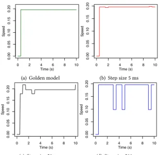
Figure 1: ModelC1 produces data v1 consumed by P1. In order to illustrate this phenomenon, we have created different time-triggered co-simulation runs where the speed of the wheel is constant (i.e.,v1 changes periodically). We have used four different setups for the co-simulation period and we have studied the corresponding impact on the speed computation according to the information retrieved by the coordinator. The results are shown in Figure 2, where we can see that smaller the time trigger period is, smaller the error is. However, this is never perfect due to the sampling of the coordinator. Additionally, this oversampling leads to useless communication points which decrease performance (see [6]), a fortiori when the wheel turns slowly (i.e., when the period ofv1 is bigger). If the model simulator supports step rejec-tion, then the accuracy problem does not hold. However, it introduces roll-backs for each 1/32 of wheel revolution and consequently a performance problem (see [9]). Finally, when the time between two switches in the output of the wheel encoder driver is not constant, the period used for the co-simulation is either pessimistic or introduce inaccuracy. To overcome these problems, we propose to let the simu-lator decide when the simulation must be stopped according to the configuration done by the coordinator. The goal is to avoid step rejection, to obtain good accuracy and to reduce as much as possible the communications between the model simulator and the coordinator.
To drive the co-simulation, we used the coordination spec-ified in Algorithm 1, where the simulation ofC1 and P1 is coordinated by using both the traditional time-triggered service (doStep) and a new event-based service (simulateUn-tilDiscontinuity). Its interface is defined as follows.
(a) Golden model (b) Step size 5 ms
(c) Step size 50 ms (d) Step size 500 ms
Figure 2: Comparison of the wheel speed between the golden model and time driven coordinator with differ-ent communication step sizes.
Algorithm 1 Coordination algorithm involving a discrete output
1: P1 := newSpeedComputationModel; 2: C1 := newW heelEncoderModel; 3: whilet ≤ tenddo
4: C1.simulateU ntilDiscontinuity( 5: v1, &tnext Event);
6: P1.doStep(t, tnext Event−t);
7: tmp = C1.дetV 1(); 8: P1.setV 1(tmp); 9: t := tnext Event; 10: end while simulateUntilDiscontinuity( in Set<Variable> monitoredVars, out time nextEventTime)
When using this function on a specific model, the model simulator monitors the assignments of each variable in the monitoredVarsset. Every time a discontinuity happens on one of these variables, the function sets nextEventTime to its current internal time and returns immediately. The function takes two parameters:
• The monitoredVars input parameter is the list of vari-ables the model simulation has to monitor, looking for a discontinuity;
• The nextEventTime output parameter returns the in-ternal simulation time when a discontinuity occurred.
RAPIDO’18, January 2018, Manchester, UK G. Liboni et al.
The main idea of the coordinator algorithm is that the coordinator asksC1 to simulate until a discontinuity is de-tected onv1. When the function returns, the coordinator knows 1) the exact time of the assignment and 2) that this is the first assignment of interest that happened between timet and tnext Event. Then the coordinator calls the doStep function onP1 (line 6) to simulate it until the time at which the discontinuity appeared inC1. Then, it retrieves the value that caused the discontinuity fromC1 and set it to P1 (line 7 and 8). By using this coordination algorithm, the number of communication points is equal to the number of disconti-nuities in the cyber model (i.e., the smallest one to retrieve all the values of the variable) and the timestamps of the discontinuities are precisely known. This simple coordina-tion provides no rollback, no overhead in the co-simulacoordina-tion execution time and perfect temporal accuracy.
3.3
Coordination of a cyber model with
input(s)
As a second example, consider a cyber modelC1 that senses the environment (e.g., a room, a CPU) and computes the temperature. Usually, in the actual implementation of such system, the environment is sensed periodically. We consider here that the environment that provides the temperature evolution is modeled by a physical modelP1 whose output is read periodically byC1 (see Figure 3). In usual time-triggered co-simulation, the co-simulation period is chosen so that the data obtained by the physical model is fresh enough when propagated to the cyber model.
Figure 3: ModelP1 produces data v1 consumed by C1. There are three drawbacks here. First, the cyber model is called several times to update its input even if this input is not required to be read internally thus wasting simula-tion time. Second, the physical model is called several times to compute fresh values that are actually not used by the cyber model. Third, there is no synchronization between the actual reading of the input by the cyber model and its update by the coordinator. This can lead to a temporal in-accuracy since the actual reading can occur at the end of a simulation step, i.e., without a fresh input. In this case, either the designer considers that the freshness of the data is not important (but that can lead to wrong simulation results !) or the designer decreases the co-simulation period and consequently decreases the performance.
As shown in the previous section, increasing the number of communication points between models and coordinator for better accuracy decreases the overall performance and therefore we aim at reducing the number of communication points without reducing accuracy.
To solve this problem, we propose to enable the simula-tion of a model until the precise time when it is ready to internally read on one of its inputs. It provides the coordina-tor with the time at which the read operation will be actually done. On the one hand it avoids unnecessary calls to the cyber model simulator; on the other hand, the coordinator can ask the physical model to compute the input data at the exact time it will be read by the cyber model (by calling the traditional doStep method with the appropriate communi-cation step size). At the next call of the cyber model, it will read the input data that has been updated specifically for it. Algorithm 2 describes the coordinator that implements such proposition. In this case,C1 is simulated first (line 4 and 5). When it returns,P1 is simulated until the reading time ofC1 (line 6). Then the value retrieved from P1 is sent to C1 (line 7 and 8).
Algorithm 2 Co-simulation Master Algorithm read opera-tion
1: P1 := newEnvFMU ;
2: C1 := newSensorDriverFMU ; 3: whilet ≤ tenddo
4: C1.simulateU ntilRead( 5: v1, &tnext Event);
6: P1.doStep(t, tnext Event−t);
7: tmp = P1.дetV 1(); 8: C1.setV 1(tmp); 9: t := tnext Event;
10: end while
To create this coordination we used a new event-based interface named simulateUntilRead, defined as follows: simulateUntilRead(
in Set<Variable> inVars, out Time& nextEventTime)
It enables the simulation of a model until it is ready to do a read operation on one of the input variables in the inVars set. The function takes two parameters:
• The inVars input parameter is a list of sensitive Vari-able for which the function should return before their communication;
• The nextEventTime output parameter provides the internal simulator time just before the read occurs.
3.4
Conditional simulation
Sometimes, input values of a model internally participate in a conditional statement. Depending on the condition, different behaviors are chosen (e.g., by using a traditional ifstatement). For instance, let us consider a simple counter C1 that increments a value v1 consumed by a model P1. Internally toP1, when v1 reaches a specific value, then P1 changes its behavior. Usually, this is implemented in co-simulation by periodically providing the input value to the
model, which checks if the value reaches the condition or not. To avoid previously presented drawbacks, a designer could use the coordinator presented in section 3.2 where the input value is provided with a good temporal precision. We go further here by defining a coordinator that asks a model to simulate until a specific condition is reached on one of its output variables. This avoids unnecessary communication points between the model simulators and the coordinator and consequently provides better performance.
The coordinator used in this case (Algorithm 3) is similar to Algorithm 1. However, during the setup phase, it retrieves the predicates fromP1 to construct the condition variables sent as a parameter ofC1 simulation.
Algorithm 3 Coordination Algorithm with Predicate
1: C1 := newEnvFMU ; 2: P1 := newSensorFMU ; 3: conds := P1.дetPredicates(); 4: condV ars := setupVars(conds); 5: whilet ≤ tenddo
6: C1.simulateU ntilCondition( 7: condV ars, &tnext Event);
8: ... (see Algorithm 1)
9: end while
This coordinator uses a new event-based interface to han-dle conditional checks:
simulateUntilCondition( Set<CondVariable> outVars, Fmu2Time& nextEventTime)
CondVariableextends the Variable structure with a Boolean predicate. Using this interface, the model providing data is simulated and each time an assignment is done on one of the variables in outVars, then the predicate is evaluated. When a predicate is evaluated to True, then the function returns. This interface can have a positive effect on per-formance provided that more information about the model internal behavior are available with respect to traditional co-simulation.
4
TOOL INTEGRATION
In this section, we present the technical background used for the experiments. We are going to present FMI, the industrial co-simulation standard, and HIFSuite, a tool suite to perform model manipulation.
4.1
FMI - Functional Mock-up Interface
FMI is a tool-independent standard framework for co-simula-tion of dynamic models. The FMI standard is managed and developed as a Modelica Association Project. FMI provides a standardized interface allowing different executable models (named FMU: Functional Mock-up Unit) to be controlled
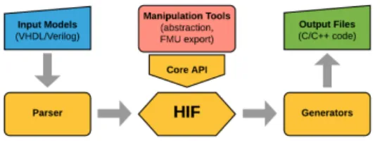
Figure 4: FMU generation flow with HIFSuite.
by an external software entity. The data exchange between models is restricted to communication points. Between two communication points (i.e., during a simulation step), the models are solved independently by each FMU simulator. The coordination is implemented by the so-called Master Algorithm (MA). FMI standard regulates the set of interfaces provided by each simulator (i.e., FMU) which are called by the master algorithm. The master algorithm is not part of the FMI standard. It can set or get the current value of an exposed variable (according to its direction) by using the standardized FMI API. This API is also used to simulate the model for a specific interval of time specified in the doStep method. In the co-simulation mode, each FMU solver decides how many computational steps should be done in that time interval to reach the desired precision.
In order to perform experiments, we implemented the proposed API as a backward compatible extension of FMI. The extended version of FMI is available on the already mentioned website.
4.2
HIFSuite
In order to drive our experiments based on both the existing and the extended FMI API, we need cyber models for which it is possible to adapt the FMU wrapper. We adopted EDALab’s HIFSuite3to make the process automatic.
HIFSuite provides tools to automatically perform sophis-ticated manipulations on models written in state-of-the-art Hardware Description Languages (HDL), like Verilog and VHDL. An HDL file is translated into a Heterogeneous Inter-mediate Format (HIF) description that can be manipulated by other HIFSuite tools that generate functionally equiv-alent C/C++ models. For our purpose, we implemented a manipulation tool to add an FMI wrapper around the model before being exported into C/C++. The resulting source code can then be used to generate an FMU as shown in Figure 4. More in detail, a front-end tool parses the input HDL file. It analyzes all the dependencies between processes in order to handle descriptions involving both synchronous and asynchronous processes. A dependency graph is gener-ated to reproduce the cycle-accurate behavior of the model. Also, when an HDL unit features an input clock signal, a
RAPIDO’18, January 2018, Manchester, UK G. Liboni et al.
clock generator process, which simulates the clock signal, is instantiated to make the model self executable. Then the model is abstracted to C/C++ and all processes and data types are converted. A special structure is created to contain a field for each input and output port of the original model. At this point, the FMU exporter tool generates the wrapper that implements the FMI Standard API. For instance, the im-plementation of the doStep method ensures that the internal clock cycles reflect the required simulation time.
The last step generates the C++ source code which must be compiled to produce a shared library and compressed to become an FMU. The process has been validated by import-ing and testimport-ing the resultimport-ing FMU into Simulink.
To support the new interfaces, HIFSuite has to generate the previously presented methods and to modify the model behavior, e.g., to stop the execution before reading a port.
5
EXPERIMENTAL RESULTS
To validate our proposal, we created three different small illustrative examples. Each example uses FMI to co-simulate two FMUs, one is a cyber FMU written in VHDL and the other one is a physical FMU written in Modelica and ex-ported using JModelica4. We extended FMI introducing the new event-based interfaces presented in section 3.
5.1
Case study #1
The first case study reproduces the system described in Sec-tion 3.2, where a cyber FMUC1 implements a wheel encoder driver and where a physical FMUP1 computes the wheel speed based on the time between the value switches of the wheel encoder. The first immediate result was that we obtain a realistic value of the wheel speed from the coordinator and soP1 computed perfectly the wheel speed, both in the case of a constant speed and in the case of a time-varying speed (see the website for numerical results). We also obtained a number of communication points between the coordinator and the FMU which was equal to the number of switches of v1 so that the implementation behaved as expected.
To compare both approaches from a performance point of view, we set up the time-triggered co-simulation in order to obtain less than 1% of error on the computed wheel speed. The error with time-triggered coordinator and a wheel with a diameter of 1 meter is characterized by equation 1:
error = 1 − π 32 ·∆t π 32 · (∆t − 2 · TTT CS) (1)
where∆t is the time between two switches of v1 and TTT CSis the time triggered co-simulation period. In a few words, the switch can occur just after a read occurs and the next switch just after the read occurs, providing a maximum
4http://www.jmodelica.org Method Time Triggered Mixed Communication Points 2000000 10000 C1 execution time (ms) 5805 4186 P1 execution time (ms) 2455 89 Table 1: Performance comparison between a time-triggered approach with less than 1% error and the proposed approach.
Method Time Triggered Mixed TTT CS(ms) 5 10 30
Communication
Points 2000 1000 334 200 C1 execution time (ns) 2123 2309 1491 1667 P1 execution time (ns) 4058 2446 850 529 Table 2: Comparison between the time triggered ap-proach with difference co-simulation period and the proposed approach.
temporal error of 2 timesTTT CS. According to this, for a switch period of 100ms (corresponding to the maximum speed of the wheel) it is required to setTTT CS to 500ns. With such settings and for a simulated time of 1000 seconds we obtained the results shown in Table 1. By reducing the number of co-simulation points, the co-simulation speed is doubled.
5.2
Case study #2
We implemented the case study described in Section 3.3, i.e., a system composed by a physical FMU that implements the temperature of an environment and a cyber FMU that implements a sensor driver. It reads periodically the value of the environment and then uses it for further computation.
We simulated this system using different periods for the time triggered co-simulation and using the proposed API. We obtained the best accuracy with the proposed approach and the performance results for 10 seconds of simulated time are summarized in Table 2.
As in the previous experiments, with a time-driven ap-proach, depending if we want to privilege temporal accuracy or performance, we have to choose a different value for the co-simulation period. If we want good temporal precision with the time triggered approach, we have to choose a small period and there is a performance drawback due to the high number of communication points. If we want to improve performance, we have to increase the co-simulation period and we obtain less accurate results due to temporal inaccu-racy. In table 2, we see that the proposed approach has the minimum communication points and like previously, the new approach has the minimum cost and a perfect accuracy.
Method Time Triggered Mixed Communication Points 20000 40
C1 execution time (ns) 4257 1653 P1 execution time (ns) 49682 479 Table 3: Comparison between the time triggered and the proposed approach an input is used in a condi-tional statement.
5.3
case study #3
In the third case, we implement the coordinator described in Section 3.4. In this experiment a cyber FMU implements a modulo counter, which is incremented periodically and reset to 0 at some points. Then, a physical FMU reads this value and change the slope of its output accordingly if the value is greater than a specific value or not. As described in 3, the coordinator starts by simulatingC1, which runs until the condition expected byP1 is reached. Then the coordinator retrieves the value fromC1 and simulates P1 until the time at which the value changes. Then the value is set toP1 and the process continues. Table 3 shows results for a simulated time of 10 seconds, using the proposed approach and the time-triggered one. The results are as expected. By reducing the number of communication points, we increase performance, here by a factor of 25. Note that with our mechanism, the point in time when the predicate becomes true is computed by the value provider and is consequently more accurate than with a time driven-triggered approach.
6
RELATED WORK
We are not the only ones to spot some limitations in FMI. For instance, [5] and [4] proposed to add static information in FMI (e.g., input/output dependencies) or to add the event type, which has the specificity to be defined only at specific points in time. These extensions are of great interest and complementary to ours. However, they did not provide any implementations or benchmark. Some other related works like [25] proposed extensions to better integrate cyber mod-els in a co-simulation. They proposed four new primitives among which one is close to ours: fmi21DoStep(stepSize, nex-tEventTime) where a FMU can be simulated for a specific amount of time and can stop if an internal event occurs, without a need to roll back. It is the same global idea than fmi2SimulateUntilDiscontinuity; however, we believe it is important to specify the variables we want to monitor since some of them can be unused or their discontinuity can be irrelevant for the system accuracy. All the other primitives introduced in [25] are either optimizations like the possibil-ity to cancel a running step (if another rejected a step) or used when the FMU can predict their future (like already proposed in [4]). Compared to all these approaches we went
a step forward by identifying situations where our new ex-tensions make simulation faster and more accurate. Also, we implemented them in a backward compatible way. We found on a FMI forum a proposal to add discrete states and time events in FMI(https://trac.fmi-standard.org/ticket/353). Their goal was to add information about the FMU to en-able the writing of a better master algorithm. We believe that such greyification of the FMUs are mandatory to help the designers (and eventually compilers) to better exploit FMU specificities. Unfortunately, their propositions consider mainly time-driven information. Still, the general idea is very interesting and may be completed to provide information allowing to choose between the time-driven API, the event-driver API or a combination of both. Finally, in order to improve performances, some papers proposed to distribute the FMUs on different hosts [12, 14]. The idea is interesting but according to previous tries on distributing time-driven simulations, we believe that introducing an event-driven API is a key enabler for a correct and efficient distributed simulation (as highlighted for years by [11, 15]).
7
CONCLUSION
We highlighted some performance and accuracy problems of time-triggered coordinators when used to co-simulate Cyber-Physical Systems. We proposed mixed event- and time-triggered coordinator to overcome these problems. We showed the benefits of the proposed approach on some small examples by developing a backward compatible extension of the FMI standard. Based on the model manipulation flow provided by the HIFSuite tool, we also implemented an FMI exporter for VHDL cyber models. We have multiple plans for future work. Technical future work will consider the full automation of the VHDL to FMU export and the improve-ment of the FMU wrapper impleimprove-mentation. Scientific future work will investigate a modeling environment that provides enough information about FMUs and their exposed variable to enable the automatic synthesis of the most efficient co-ordinator. For this purpose, we are currently exploring the use of a dedicated language based on a mix between logical and physical time.
REFERENCES
[1] Muhammad Usman Awais, Peter Palensky, Atiyah Elsheikh, Edmund Widl, and Stifter Matthias. 2013. The high level architecture RTI as a master to the functional mock-up interface components. In Computing, Networking and Communications (ICNC), 2013 International Conference on. IEEE, 315–320.
[2] Jens Bastian, Christop Clauß, Susann Wolf, and Peter Schneider. 2011. Master for co-simulation using FMI. In Proceedings of the 8th Inter-national Modelica Conference; March 20th-22nd; Technical Univeristy; Dresden; Germany. Linköping University Electronic Press, 115–120. [3] Frédéric Boussinot and Robert De Simone. 1991. The ESTEREL language.
Proc. IEEE 79, 9 (1991), 1293–1304.
[4] David Broman, Christopher Brooks, Lev Greenberg, Edward A Lee, Michael Masin, Stavros Tripakis, and Michael Wetter. 2013. Determinate composition of FMUs for co-simulation. In Proceedings of the Eleventh ACM International Conference on Embedded Software. IEEE Press, 2.
RAPIDO’18, January 2018, Manchester, UK G. Liboni et al.
[5] David Broman, Lev Greenberg, Edward A. Lee, Michael Masin, Stavros Tripakis, and Michael Wetter. 2014. Requirements for Hybrid Cosimu-lation. Technical Report UCB/EECS-2014-157. EECS Department, Uni-versity of California, Berkeley. to appear in HSCC, Seattle, WA, April 14-16, 2015.
[6] Stefano Centomo, Julien Deantoni, and Robert De Simone. 2016. Using SystemC Cyber Models in an FMI Co-Simulation Environment. In 19th Euromicro Conference on Digital System Design 31 August - 2 Septem-ber 2016 (19th Euromicro Conference on Digital System Design), Vol. 19. Limassol, Cyprus. https://doi.org/10.1109/DSD.2016.86
[7] Benoit Combemale, Cédric Brun, Joël Champeau, Xavier Crégut, Julien Deantoni, and Jérome Le Noir. 2016. A Tool-Supported Approach for Concurrent Execution of Heterogeneous Models. In 8th European Con-gress on Embedded Real Time Software and Systems (ERTS 2016). [8] Benoit Combemale, Julien Deantoni, Benoit Baudry, Robert B. France,
Jean-Marc Jézéquel, and Jeff Gray. 2014. Globalizing Modeling Lan-guages. IEEE Computer (June 2014), 10–13. https://hal.inria.fr/ hal-00994551
[9] Fabio Cremona, Marten Lohstroh, Stavros Tripakis, Christopher Brooks, and Edward A. Lee. 2016. FIDE - An FMI Integrated Development Environment. In Symposium on Applied Computing.
[10] Julien Deantoni, Cédric Brun, Benoit Caillaud, Robert B. France, Gabor Karsai, Oscar Nierstrasz, and Eugene Syriani. 2015. Domain Global-ization: Using Languages to Support Technical and Social Coordination. Springer International Publishing, Cham, 70–87. https://doi.org/10.1007/ 978-3-319-26172-0_5
[11] Colin Fidge. 1991. Logical time in distributed computing systems. Com-puter 24, 8 (1991), 28–33.
[12] Virginie Galtier, Stephane Vialle, Cherifa Dad, Jean-Philippe Tavella, Jean-Philippe Lam-Yee-Mui, and Gilles Plessis. 2015. FMI-based Dis-tributed Multi-simulation with DACCOSIM. In Proceedings of the Sym-posium on Theory of Modeling & Simulation: DEVS Integrative M&S Symposium (DEVS ’15). Society for Computer Simulation International, San Diego, CA, USA, 39–46.
[13] David Garlan and Mary Shaw. 1993. An introduction to software archi-tecture. Advances in software engineering and knowledge engineering 1, 3.4 (1993).
[14] Abir Ben Khaled, Mongi Ben Gaid, Nicolas Pernet, and Daniel Simon. 2014. Fast multi-core co-simulation of Cyber-Physical Systems: Applica-tion to internal combusApplica-tion engines. SimulaApplica-tion Modelling Practice and Theory 47 (2014), 79 – 91. https://doi.org/10.1016/j.simpat.2014.05.002 [15] Leslie Lamport. 1978. Time, clocks, and the ordering of events in a
distributed system. Commun. ACM 21, 7 (1978), 558–565.
[16] Matias Ezequiel Vara Larsen, Julien Deantoni, Benoit Combemale, and Frédéric Mallet. 2015. A behavioral coordination operator language (BCOoL). In Model Driven Engineering Languages and Systems (MODELS), 2015 ACM/IEEE 18th International Conference on. IEEE, 186–195. [17] Matias Ezequiel Vara Larsen, Julien Deantoni, Benoit Combemale, and
Frédéric Mallet. 2015. A Model-Driven Based Environment for Auto-matic Model Coordination. In Models 2015 demo and posters. [18] Edward A Lee. 2008. Cyber physical systems: Design challenges. In
Object Oriented Real-Time Distributed Computing (ISORC), 2008 11th IEEE International Symposium on. IEEE, 363–369.
[19] Nenad Medvidovic and Richard N Taylor. 1997. A framework for classi-fying and comparing architecture description languages. ACM SIGSOFT Software Engineering Notes 22, 6 (1997), 60–76.
[20] Modelisar. 2014. FMI for Model Exchange and Co-Simulation. (July 2014). https://fmi-standard.org/downloads#version2
[21] Himanshu Neema, Jesse Gohl, Zsolt Lattmann, Janos Sztipanovits, Gabor Karsai, Sandeep Neema, Ted Bapty, John Batteh, Hubertus Tummescheit, and Chandraseka Sureshkumar. 2014. Model-based integration platform for FMI co-simulation and heterogeneous simulations of cyber-physical systems. In Proceedings of the 10 th International Modelica Conference; Lund; Sweden. Linköping University Electronic Press, 235–245. [22] George A Papadopoulos and Farhad Arbab. 1998. Coordination models
and languages. Advances in computers 46 (1998), 329–400.
[23] Vitaly Savicks, Michael Butler, and John Colley. 2014. Co-simulating Event-B and continuous models via FMI. In Proceedings of the 2014 Summer Simulation Multiconference. Society for Computer Simulation International, 37.
[24] Tom Schierz, Martin Arnold, and Christoph Clauß. 2012. Co-simulation with communication step size control in an FMI compatible master algorithm. In Proceedings of the 9th International MODELICA Conference;
Munich; Germany. Linköping University Electronic Press, 205–214. [25] Jean-Philippe Tavella, Mathieu Caujolle, Charles Tan, Gilles Plessis,
Mathieu Schumann, Stéphane Vialle, Cherifa Dad, Arnaud Cuccuru, and Sébastien Revol. 2016. Toward an Hybrid Co-simulation with the FMI-CS Standard. (April 2016). https://hal-centralesupelec.archives-ouvertes. fr/hal-01301183 Research Report.
[26] S. Tripakis. 2015. Bridging the semantic gap between heterogeneous modeling formalisms and FMI. In 2015 International Conference on Embedded Computer Systems: Architectures, Modeling, and Simulation (SAMOS). 60–69. https://doi.org/10.1109/SAMOS.2015.7363660 [27] Bert Van Acker, Joachim Denil, Hans Vangheluwe, and Paul De
Meu-lenaere. 2015. Generation of an Optimised Master Algorithm for FMI Co-simulation. In Proceedings of the Symposium on Theory of Modeling & Simulation: DEVS Integrative M&S Symposium (DEVS ’15). Society for Computer Simulation International, San Diego, CA, USA, 205–212. [28] Baobing Wang and John S. Baras. 2013. HybridSim: A Modeling and
Co-simulation Toolchain for Cyber-physical Systems. In Proceedings of the 2013 IEEE/ACM 17th International Symposium on Distributed Simu-lation and Real Time Applications (DS-RT ’13). IEEE Computer Society, Washington, DC, USA, 33–40. https://doi.org/10.1109/DS-RT.2013.12