Automating sized-type inference for complexity analysis

HAL Id: hal-01639200

https://hal.inria.fr/hal-01639200

Submitted on 20 Nov 2017

HAL is a multi-disciplinary open access

archive for the deposit and dissemination of

sci-entific research documents, whether they are

pub-lished or not. The documents may come from

teaching and research institutions in France or

abroad, or from public or private research centers.

L’archive ouverte pluridisciplinaire HAL, est

destinée au dépôt et à la diffusion de documents

scientifiques de niveau recherche, publiés ou non,

émanant des établissements d’enseignement et de

recherche français ou étrangers, des laboratoires

publics ou privés.

Martin Avanzini, Ugo Dal Lago

To cite this version:

Martin Avanzini, Ugo Dal Lago. Automating sized-type inference for complexity analysis. Proceedings

of the ACM on Programming Languages, ACM, 2017, 1 (ICFP), pp.1 - 29. �10.1145/3110287�.

�hal-01639200�

43

MARTIN AVANZINI,

UGO DAL LAGO,

This paper introduces a new methodology for the complexity analysis of higher-order functional programs, which is based on three ingredients: a powerful type system for size analysis and a sound type inference procedure for it, a ticking monadic transformation, and constraint solving. Noticeably, the presented method-ology can be fully automated, and is able to analyse a series of examples which cannot be handled by most competitor methodologies. This is possible due to the choice of adopting an abstract index language and index polymorphism at higher ranks. A prototype implementation is available.

CCS Concepts: •Theory of computation → Program analysis; Automated reasoning; Equational logic and rewriting; • Software and its engineering → Functional languages;

ACM Reference format:

Martin Avanzini and Ugo Dal Lago. 2017. Automating Sized-Type Inference for Complexity Analysis.Proc. ACM Program. Lang. 1, 1, Article 43 (September 2017), 28 pages.

https://doi.org/10.1145/3110287

1 INTRODUCTION

Programs can be incorrect for very different reasons. Modern compilers are able to detect many

syntactic errors, including type errors. When the errors are semantic, namely when the program is

well-formed but does not compute what it should, traditional static analysis methodologies like

abstract interpretation or model checking could be of help. When a program is functionally correct

but performs quite poorly in terms of space and runtime behaviour, evendefining the property of interest is very hard. If the units of measurement in which program performances are measured are

close to the physical ones, the problem can only be solved if the underlying architecture is known,

due to the many transformation and optimisation layers which are applied to programs. One then

obtains WCET techniques [Wilhelm et al. 2008], which indeed need to deal with how much machine

instructions cost when executed by modern architectures (including caches, pipelining, etc.), a task

which is becoming even harder with the current trend towards multicore architectures.

As an alternative, one can analyse theabstract complexity of programs. As an example, one can take the number of evaluation steps to normal form, as a measure of the underlying program’s

execution time. This can be accurate if the actual time complexityof each instruction is kept low, and has the advantage of being independent from the specific hardware platform executing the program

at hand, which only needs to be analysedonce. A variety of verification techniques have indeed been defined along these lines, from type systems to program logics, to abstract interpretation,

see [Aspinall et al. 2007; Albert et al. 2013; Sinn et al. 2014; Hoffmann et al. 2017].

If we restrict our attention to higher-order functional programs, however, the literature becomes

sparser. There seems to be a trade-off between allowing the user full access to the expressive

power of modern, higher-order programming languages, and the fact that higher-order parameter

passing is a mechanism which intrinsically poses problems to complexity analysis: how big is a

certain (closure representation of a) higher-order parameter? If we focus our attention on automatic

techniques for the complexity analysis of higher-order programs, the literature only provides very

2017. 2475-1421/2017/9-ART43

few proposals [Vasconcelos et al. 2008; Avanzini et al. 2015; Hoffmann et al. 2017], which we will

discuss in Section 2 below.

One successful approach to automatic verification oftermination properties of higher-order functional programs is based onsized types [Hughes et al. 1996], and has been shown to be quite robust [Barthe et al. 2008]. In sized types, a type carries not only some information about the kind of each object, but also about its size, hence the name. This information is then exploited when requiring that recursive calls are done on arguments ofstrictly smaller size, thus enforcing termination. Estimating the size of intermediate results is also a crucial aspect of complexity analysis,

but up to now the only attempt of using sized types for complexity analysis is due to Vasconcelos

et al. [2008], and confined to space complexity. If one wants to be sound for time analysis, size

types need to be further refined, e.g., by turning them into linear dependently types [Dal Lago et al.

2011].

In this paper, we take a fresh look at sized types by introducing a new type system which is

sub-stantially more expressive than the traditional one. This is possible due to the presence ofarbitrary rank index polymorphism: functions that take functions as their argument can be polymorphic in their size annotation. The introduced system is then proved to be a sound methodology forsize analysis, and a type inference algorithm is given and proved sound and relatively complete. Finally,

the type system is shown to be amenable to time complexity analysis by a ticking monadic

trans-formation. A prototype implementation is available, see below for more details. More specifically,

this paper’s contributions can be summarized as follows:

· We show that size types can be generalised so as to encompass a notion of index polymorphism, in which (higher-order subtypes of ) the underlying type can be universally quantified. This

allows for a more flexible treatment of higher-order functions. Noticeably, this is shown to

preserve soundness (i.e., subject reduction), the minimal property one expects from such a type

system. On the one hand, this is enough to be sure that types reflect the size of the underlying

program. On the other hand, termination is not enforced anymore by the type system, contrarily

to, e.g., the system of Hughes et al. [1996]. In particular, we do not require that recursive calls

are made on arguments of smaller size. All this is formulated on a language of applicative

programs, introduced in Section 4, and will be developed in Section 5. Nameless functions (i.e., λ-abstractions) are not considered for brevity, as these can be easily lifted to the top-level. · The type inference problem is shown to be (relatively) decidable by giving in Section 6 an

algorithm which, given a program, produces in output candidate types for the program, together

with a set of integer index inequalities which need to be checked for satisfiability. This style

of results is quite common in similar kinds of type systems. What is uncommon though, at

least in the context of sized types, is that we do not restrict ourselves to a particular algebra

in which sizes are expressed. Indeed, many of the more advanced sized type systems are

restricted to the successor algebra [Blanqui et al. 2005; Abel et al. 2016]. This is often sufficient

in the context of termination analysis, where one is interested in determining which recursion

parameters decrease. Here, the programs runtime will be expressed in this algebra, and thus a

more expressive algebra is required.

· The polymorphic sized type system, by itself, does not guarantee any complexity-theoretic property on the typed program, except for thesize of the output being bounded by a function on the size of the input, itself readable from the type. Complexity analysis of a programP can however be seen as a size analysis of another program ˆP which computes not only P, but its complexity. This transformation, called theticking transformation, has already been studied in similar settings [Danner et al. 2015], but this study has never been automated. The ticking

· Contrarily to many papers from the literature, we spent considerable efforts on devising a system that is susceptible to automation with current technology. Moreover, we have taken care

not only of constraintinference, but also of constraint solving. To demonstrate the feasibility of our approach, we have built a prototype which implements type inference, resulting in a set of

constraints. To deal with the resulting constraints, we have also built a constraint solver on top

of state-of-the-art SMT solvers. All this, together with some experimental results, are described

in detail in Section 8.

An extended version with more details is available as supplementary material.

2 A BIRD EYE’S VIEW ON INDEX-POLYMORPHIC SIZED TYPES

In this section, we will motivate the design choices we made when defining our type system through

some examples. This can also be taken as a gentle introduction to the system for those readers

which are familiar with functional programming and type theory. Our type system shares quite

some similarities with the seminal type system introduced by Hughes et al. [1996] and similar ones

[Vasconcelos et al. 2008; Barthe et al. 2008], but we try to keep presentation as self-contained as

possible.

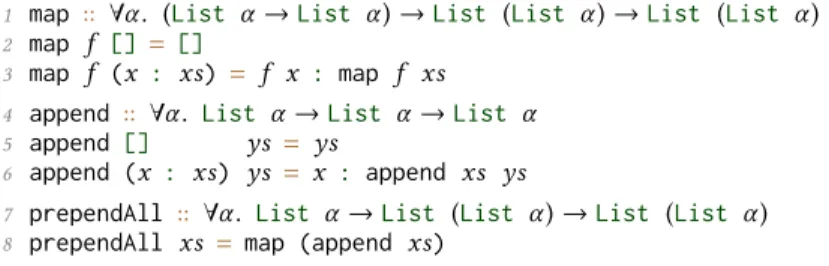
Basics. We work with functional programs over a fixed set of inductive datatypes, e.g.Natfor natural numbers andListα for lists over elements of type α . Each such datatype is associated with a set of typedconstructors, below we will use the constructors 0 ::Nat,Succ ::Nat →Natfor naturals, and the constructor [ ] ::∀α .Listα and the infix constructor(:) :: ∀α. α →Listα →

Listα for lists. Sized types refine each such datatype into a family of datatypes indexed by natural numbers, theirsize. E.g., toNatandListα we associate the familiesNat0,Nat1,Nat2, . . . andList0α,List1α,List2α, . . . , respectively. An indexed datatype such asList_n Nat_m then represents lists of lengthn, over naturals of size m.

A functionf will then be given a polymorphic type ∀⃗α . ∀⃗i. τ → ζ . Whereas the variables ⃗α range over types, the variables⃗i range over sizes. Datatypes occurring in the types τ and ζ will be indexed by expressions over the variables⃗i. E.g., the append function can be attributed the sized type∀α . ∀ij.List_iα →List_j α →List_i+jα .

Soundness of our type-system will guarantee that when append is applied to lists of lengthn and m respectively, it will yield a list of size n+ m, or possibly diverge. In particular, our type system is not meant to guarantee termination, and complexity analysis will be done via the aforementioned

ticking transformation, to be described later. As customary in sized types, we will also integrate a

subtyping relationτ ⊑ ζ into our system, allowing us to relax size annotations to less precise ones. This flexibility is necessary to treat conditionals where the branches are attributed different sizes,

or, to treat higher-order combinators which are used in multiple contexts.

Our type system, compared to those from the literature, has its main novelty in polymorphism,

but is also different in some key aspects, addressing intensionality but also practical considerations

towards type inference. In the following, we shortly discuss the main differences.

Canonical Polymorphic Types. We allow polymorphism over size expressions, but put some syntactic restrictions on function declarations: In essence, we disallow non-variable size annotations

directly to the left of an arrow, and furthermore, all these variables must be pairwise distinct.

We call such types canonical. The first restriction dictates that e.g.half :: ∀i.Nat2_·i → Nat_i has to be written ashalf :: ∀i.Nat_i → Nat_i/2. The second restriction prohibits e.g. the type declarationf :: ∀i.Nat_i → Nat_i → τ , rather, we have to declare f with a more general type ∀ij.Nat_i →Nat_j →τ′_{. The two restrictions considerably simplify the inference machinery when}

1 rev :: ∀α . ∀ij. Listi α →Listj α →List_i+j α

2 rev [] ys = ys

3 rev (x : xs) ys = rev xs (x : ys)

4 reverse :: ∀α . ∀i. List_i α →List_i α

5 reverse xs =rev xs []

Fig. 1. Sized type annotated tail-recursive list reversal function.

unification based mechanism, a matching mechanism suffices. Unlike in [Hughes et al. 1996], where

indices are formed over naturals and addition, we keep the index language abstract. This allows for

more flexibility, and ultimately we can capture more programs. Indeed, having the freedom of not

adopting a fixed index language is known to lead towards completeness [Dal Lago et al. 2011].

Polymorphic Recursion over Sizes. Type inference in functional programming languages, such asHaskell or OCaml, is restricted to parametric polymorphism in the form oflet-polymorphism. Recursive definitions are checked under a monotype, thus, types cannot change between recursive

calls. Recursive functions that require full parametric polymorphism [Mycroft et al. 1984] have to

be annotated in general, as type inference is undecidable in this setting.

Let-polymorphism poses a significant restriction in our context, because sized types considerably

refine upon simple types. Consider for instance the usual tail-recursive definition of list reversal

depicted in Figure 1. With respect to the annotated sized types, in the body of the auxiliary function rev defined on line 3, the type of the second argument to rev will change fromList_j α (the assumed type ofys) toList_j+1α (the inferred type of x : ys). Consequently, rev is not typeable under a monomorphic sized type. Thus, to handle even such very simple functions, we will have to

overcome let-polymorphism, on the layer of size annotations. To this end, conceptually we allow

also recursive calls to be given a type polymorphic over size variables. This is more general than

the typing rule for recursive definitions found in more traditional systems [Hughes et al. 1996;

Barthe et al. 2008].

Higher-ranked Polymorphism over Sizes. In order to remain decidable, classical type inference systems work on polymorphic types inprenex form ∀⃗α .τ , where τ is quantifier free. In our context, it is often not enough to give a combinator a type in prenex form, in particular when the combinator

uses a functional argument more than once. All uses of the functional argument have to be given

thenthe same type. In the context of sized types, this means that functional arguments can be applied only to expressions whose attributed size equals. This happens for instance in recursive

combinators, but also non-recursive ones such as the functiontwice f x = f (f x). A strong type-system would allow us to type the expressiontwice Succ with a sized typeNat_c →Nat_c+2. A (specialised) type in prenex form fortwice, such as

twice :: ∀i.(Nati →Nat_i+1) →Nati →Nat_i+2,

would immediately yield the mentioned sized type fortwice Succ. However, we will not be able to typetwice itself, because the outer occurrence off would need to be typed asNat_i+1 →Nat_i+2, whereas the type oftwice dictates thatf has typeNat_i →Nat_i+1.

The way out is to allow polymorphic types of rankhigher than one when it comes to size variables, i.e. to allow quantification of size variables to the left of an arrow at arbitrary depth. Thus, we can

declare

twice :: ∀i.(∀j.Nat_j →Nat_j+1) →Nat_i →Nat_i+2.

As above, this allows us to type the expressiontwice Succ as desired. Moreover, the inner quantifier permits the two occurrences of the variablef in the body of twice to take typesNat_i →Nat_i+1 andNat_i+1→Nat_i+2respectively, and thustwice is well-typed.

1 foldr :: ∀α β . ∀jkl . (∀i. α →List_i β →List_i+j β) →List_k β →List_l α →List_{l ·j+k} β

2 foldr f b [] =b

3 foldr f b (x : xs) = f x (foldr f b xs)

4 product :: ∀α β . ∀ij. List_i α →List_j β →List_{i ·j} (α × β)

5 product ms ns =foldr (λ m ps. foldr (λ n. (:) (m,n)) ps ns) [] ms Fig. 2. Sized type annotated program computing the cross-product of two lists.

A Worked Out Example. We conclude this section by giving a nontrivial example. The sized type annotated program is given in Figure 2. The functionproduct computes the cross-product [(m, n) | m ∈ ms, n ∈ ns ] for two given lists ms and ns. It is defined in terms of two folds. The inner fold appends, for a fixed elementm, the list [(m, n) | n ∈ ns ] to an accumulator ps, the outer fold traverses this function over all elementsm from ms.

In a nutshell, checking that a functionf is typed correctly amounts to checking that all its defining equations are well-typed, i.e. under the assumption that the variables are typed according

to the type declaration off, the right-hand side of the equation has to be given the corresponding return-type. Of course, all of this has to take pattern matching into account. Let us illustrate this on

the recursive equation offoldr given in Line 3 in Figure 2. Throughout the following, we denote by s : τ that the term s has type τ . To show that the equation is well-typed, let us assume the following types for arguments: f : ∀i. α → List_i β → List_i+j β, b :List_k β, x : α and xs :List_m α for arbitrary size-indicesj, k, m. Under these assumptions, the left-hand side has typeList_(m+1)·j+kβ, taking into account that the recursion parameterx : xs has size m+ 1. To show that the equation is well-typed, we verify that the right-hand side can be attributed the same sized type.

1. We instantiate the polymorphic type offoldr and derive

foldr :(∀i. α →List_i β →List_i+jβ) →List_k β →List_mα →List_{m ·j+k}β ; 2. from this and the above assumptions we getfoldrf b xs :List_{m ·j+k} β;

3. by instantiating the quantified size variablei in the assumed type of f with the index term m · j+ k we get f : α →List_{m ·j+k}β →List_{(m ·j+k)+j} β;

4. from the last two steps we finally getf x(foldr f b xs) :List_(m+1)·j+k β.

We will not explain the type checking of the remaining equations, but revisit this example in

Section 8.

3 ON RELATED WORK

Since the first inception in the seminal paper of Hughes et al. [1996], the literature on sized types

has grown to a considerable extent. Indeed, various significantly more expressive systems have

been introduced, with the main aim to enlarge the class of typable (and thus proved terminating)

programs. For instance, Blanqui et al. [2005] introduced a novel sized type system on top of the calculus of algebraic construction.

Notably, it has been shown that for size indices over the successor algebra, type checking is

decidable [Blanqui et al. 2005]. The system is thus capable of expressing additive relations between

sizes. In the context of termination analysis, where one would like to statically detect that a

recursion parameter decreases in size, this is sufficient. In this line of research falls also more recent

work of Abel et al. [2016], where a novel sized type system for termination analysis on top ofF_ωis proposed. Noteworthy, this system has been integrated in the dependently typed languageAgda.

Type systems related to sized types have been introduced and studied not only in the context of

termination analysis, but also for size and complexity analysis of programs. One noticeable example

is the series of work by Shkaravska et al. [2009], which aims at size analysis but which is limited to

However, the system is inherentlysemi-automatic. Related to this is also the work by Danielsson et al. [2008], whose aim is again complexity analysis, but which is not fully automatable and limited

to linear bounds. If one’s aim is complexity analysis of higher-order functional programs, achieving

a form of completeness is indeed possible by linear dependent types [Dal Lago et al. 2011, 2014].

While the front-end of this verification machinery is fully-automatable [Dal Lago et al. 2013], the

back-end is definitely not, and this is the reason why this paper should be considered a definite

advance over this body of work. Our work is also related to that of?, which uses a combination of runtime and size analysis to reason about the complexity of functional programs expressed as

interaction nets.

Our work draws inspiration from Danner et al. [2015]. In this work, the complexity analysis of

higher-order functional programs, defined in a system akin to Gödel’sT enriched with inductive types, is studied. A ticking transformation is used to instrument the program with a clock, recurrence

relations are then extracted from the ticked version that express the complexity of the input program.

Conceptually, our ticking transformation is identical to the one defined by Danner et al., and differs

only in details to account for the peculiarities of the language that we are considering. In particular,

our simulation theorem, Theorem 7.3, has an analogue in [Danner et al. 2015]. The proof in the

present work is however more delicate, as our language admits arbitrary recursion and programs

may thus very well diverge. To our best knowledge, no attempts have been made so far to automate

solving of the resulting recurrences.

In contrast, Hoffmann et al. refine in a series of works the methodology of Jost et al. [2010]

based onTarjan’s amortised resource analysis. This lead to the development of RAML [Hoffmann et al. 2012], a fully fledged automated resource analysis tool. Similar to the present work, the analysis is

expressed as a type system. Data types are annotated bypotentials, inference generates a set of linear constraints which are then solved by an external tool. This form of analysis can not only deal

with non-linear bounds [Hoffmann et al. 2011], but it also demonstrates that type based systems are

relatively stable under language features such as parallelism [Hoffmann et al. 2015] or imperative

features [Hoffmann et al. 2015]. In more recent work [Hoffmann et al. 2017], the methodology

has been lifted to the higher-order case andRAML can now interface with Inria’s OCaml compiler. Noteworthy, some of the peculiarities of this compiler are taken into account. The overall approach

is in general incomparable to our methodology. Whilst it seems feasible, our method neither takes

amortisation into account nor does our prototype interface with a industrial strength compiler. On

the other hand, our system can properly account for closures, whereas inherent to the methodology

underlyingRAML, closures can only be dealt with in a very restricted form. We return to this point in Section 8 within our experimental assessment.

There are also connections to the work of Avanzini et al. [2015], where a complexity preserving

transformation from higher-order to first-order programs is proposed. This transformation works

by a form of control-flow guided defunctionalisation. Furthermore, a variety of simplification

techniques, such as inlining and narrowing, are employed to make the resulting first-order program

susceptible to an automated analysis. The complete procedure has been implemented in the tool HoCA, which relies on the complexity analyser TCT [Avanzini et al. 2016] to analyse the resulting first-order program. Unlike for our system, it is unclear whether the overall method can be used to

derive precise bounds.

4 APPLICATIVE PROGRAMS AND SIMPLE TYPES

We restrict our attention to a small prototypical, strongly typed functional programming language.

For the sake of simplifying presentation, we impose a simple, monomorphic, type system on

programs, which does not guarantee anything except a form of type soundness. We will only later

ML-style polymorphic type setting. Here, such an extension would only distract from the essentials.

Indeed, our implementation (described in Section 8) allows polymorphic function definitions.

Statics. Let B denote a finite set of base types B, C, . . . . Simple types are inductively generated fromB ∈ B:

(simple types) τ , ρ, ξ ::= B | τ × ρ | τ → ρ .

We follow the usual convention that→ associates to the right. Let X denote a countably infinite set ofvariables, ranged over by metavariables like x, y. Furthermore, let F and C denote two disjoint sets of symbols, the set offunctions and constructors, respectively, all pairwise distinct with elements fromX. Functions and constructors are denoted in teletype font. We keep the convention that functions start with a lower-case letter, whereas constructors start with an

upper-case letter. Each symbols ∈ X ∪ F ∪ C has a simple type τ , and when we want to insist on that, we writesτ instead of justs. Furthermore, each symbol sτ1→···→τn→ρ _{∈ F ∪ C is associated with a}

natural numberar(s ) ≤ n, its arity. The set of terms, patterns, values and data values over functions f ∈ F , constructors C ∈ C and variablesx ∈ X is inductively generated as follows. Here, each term receives implicitly a type, in Church style. Below, we employ the usual convention that application

associates to the left.

(terms) s, t ::= xτ variable

| fτ function

| Cτ constructor

|(sτ →ρtτ)ρ application

|(sτ, tρ)τ ×ρ pair constructors |(let (xτ, yρ) = sτ ×ρin tξ)ξ pair destructor; (patterns) p, q ::= xτ | Cτ1→···τn→B_pτ1 1 · · ·p τn n ; (values) u, v ::= Cτ1→···→τn→τ_uτ1 1 · · ·u τn n | fτ1→···→τm→τm+1→τ _uτ1 1 · · ·u τm m |(uτ,vρ)τ ×ρ ; (data values) d ::= CB1→···→Bn+1 d1· · ·dn.

The presented operators are all standard, except the pair destructorlet (x, y)= s in t which binds the variablesx and y to the two components of the result of s in t . The set of free variablesFVar(s ) of a terms is defined in the usual way. IfFVar(s )= ∅, we call s ground. A term s is called linear, if each variable occurs at most once ins. A substitution θ is a finite mapping from variables xτ to termssτ. The substitution mapping⃗x= x1, . . . , xnto⃗s= s1, . . . , sn, respectively, is indicated with

{s1, . . . , sn/x1, . . . , xn} or {⃗s/⃗x} for short. The variables ⃗x are called the domain of θ . We denote by

sθ the application of θ to s. Let-bound variables are renamed to avoid variable capture.

AprogramP over functions F and constructors C defines each function f ∈ F through a finite set ofequations lτ = rτ, wherel is of the form f p1 · · ·p_{ar(f )}. We put the usual restriction on

equations that each variable occurs at most once inl, i.e. that l is linear, and that the variables of the right-hand side r are all included in l. To keep the semantics short, we do not impose any order on the equations. Instead, we require that left-hand sides definingf are all pairwise non-overlapping. This ensures that our programming model is deterministic.

Some remarks are in order before proceeding. As standard in functional programming, only

values of base type can be destructed by pattern matching. In a pattern, a constructor always needs

This would unnecessarily complicate some key definitions in later sections. Instead, a dedicated

destructorlet (x, y)= s in t is provided. We also excluded λ-abstractions from our language, for brevity, as these can always be lifted to the top-level. Similarly, conditionals and case-expressions

would not improve upon expressivity.

Dynamics. We impose a call-by-value semantics on programsP. Evaluation contexts are defined according to the following grammar:

E ::= 2τ _|(Eτ →ρ_sτ₎ρ _|(sτ →ρ_Eτ₎ρ _{| (E}τ_{, s}ρ₎τ ×ρ _|(sτ_{, E}ρ₎τ ×ρ _{|(let (x}τ_{, y}ρ_{) = E}τ ×ρ_{in s}ξ₎ξ _.

As with terms, type annotations will be omitted from evaluation contexts whenever this does not

cause ambiguity. WithE[sτ] we denote the term obtained by replacing thehole2τ inE by sτ. The one-stepcall-by-value reduction relation −→_P, defined over ground terms, is then given as the closure over all evaluation contexts, of the following two rules:

fp1 · · ·pn = r ∈ P

(f p1 · · ·pn){⃗u/⃗x} −→_Pr {⃗u/⃗x} let (x, y)= (u,v) in t −→_Pt {u, v/x, y}

We denote by→−∗

Pthe transitive and reflexive closure, and likewise,→−Pℓdenotes theℓ-fold

composi-tion of→−

P.

Notice that reduction simply gets stuck if pattern matching in the definition off is not exhaustive. We did not specify a particular reduction order, e.g., left-to-right or right-to-left. Reduction itself is

thus non-deterministic, but this poses no problem since programs arenon-ambiguous: not only are the results of a computation independent from the reduction order, but also reduction lengths

coincide.

Proposition 4.1. All normalising reductions of s have the same length and yield the same result, i.e. if s −→m_P u and s −→n_Rv then m= n and u = v.

To define theruntime-complexity ofP, we assume a single entry point to the program via a first-order function mainB1→···→Bk→Bn, which takes as input data values and also produces a data value as output. The (worst-case) runtime-complexity ofP then measures the reduction length of main in the sizes of the inputs. Here, the size|d | of a data value is defined as the number of constructor in d. Formally, the runtime-complexity function ofP is defined as the function rc_{P: N × · · · × N → N}∞:

rc_P(n₁, . . . , n_k) := sup{ℓ | ∃d₁, . . . , d_k. main d₁ · · ·d_k→−ℓ

Ps and |di|⩽ ni} ..

We emphasise that the runtime-complexity function defines a cost model that is invariant to

traditional models of computation, e.g., Turing machines [Dal Lago et al. 2009; Avanzini et al. 2010].

5 SIZED TYPES AND THEIR SOUNDNESS

This section is devoted to introducing the main object of study of this paper, namely a sized type

system for the applicative programs that we introduced in Section 4. We have tried to keep the

presentation of the relatively involved underlying concepts as simple as possible.

5.1 Indices

As a first step, we make the notion ofsize index, with which we will later annotate data types, precise. LetG denote a set of first-order function symbols, theindex symbols. Any symbolf ∈ G is associated with a natural numberar(f), its arity. The set of index terms is generated over a countable infinite set ofindex variables i ∈ V and index symbolsf ∈ G .

We denote byVar(a) ⊂ V the set of variables occurring in a. Substitutions mapping index variables to index terms are calledindex substitutions. With ϑ we always denote an index substitution. We adopt the notions concerning term substitutions to index substitutions from the previous section.

Throughout this section,G is kept fixed. Meaning is given to index terms through aninterpretation J , that maps everyk-aryf ∈ G to a (total) and weakly monotonic functionJf KJ : N

ar(f) _{→ N.}

We suppose thatG always contains a constant 0, a unary symbols, and a binary symbol+ which we write in infix notation below. These are always interpreted as zero, the successor function and

addition, respectively. Our index language encompasses the one of Hughes et al. [1996], where

linear expressions over natural numbers are considered. The interpretation of an index terma, under anassignment α : V → N and an interpretation J , is defined recursively in the usual way: Ji K

α

J := α (i) andJf (a1, . . . , ak)_Kα_J :=_JfKJ(_Ja1_Kα_J, . . . ,_Jak_Kα_J). We define a ≤J b if_JaKα_J ≤_{Jb K}α_J

holdsfor all assignments α . The following lemma collects useful properties of the relation ≤_J. Lemma 5.1.

1. The relation ≤J is reflexive, transitive and closed under substitutions, i.e. a ≤J b implies aϑ ≤J

bϑ .

2. If a ≤J b then c {a/i} ≤J c {b/i} for each index term c.

3. If a ≤J b then a{0/i} ≤J b.

4. If a ≤J b and i < Var(a) then a ≤J b{c/i} for every index term c.

5.2 Sized Types Subtyping and Type Checking

The set ofsized types is given by annotating occurrences of base types in simple types with index termsa, possibly introducing quantification over index variables. More precise, the sets of (sized) monotypes, (sized) polytypes and (sized) types are generated from base types B, index variables ⃗i and index termsa as follows:

(monotypes) τ , ζ ::= Ba |τ × ζ | ρ → τ , (polytypes) σ ::= ∀⃗i. ρ → τ , (types) ρ ::= τ | σ . TypesB_aare calledindexed base types. We keep the convention that the arrow binds stronger than quantification. Thus in a polytype∀⃗i. ρ → τ the variables ⃗i are bound in ρ and τ . We will sometimes write a monotypeτ as ∀ϵ . τ . This way, every type ρ can given in the form ∀⃗i. τ . The skeleton of a typeρ is the simple type obtained by dropping quantifiers and indices. The setsFVar+(·) and FVar−_{(·), of free variables occurring in positive and negative positions, respectively, are defined}

in the natural way. The set of free variables inρ is denoted byFVar(ρ). We consider types equal up toα -equivalence. Index substitutions are extended to sized types in the obvious way, using α -conversion to avoid variable capture.

We denote byρ ·⩾ τ that the monotype τ is obtained by instantiating the variables quantified in ρ with arbitrary index terms, i.e. if ρ= ∀⃗i.ζ then τ = ζ {⃗a/⃗i} for some index terms ⃗a. Notice that by our conventionτ = ∀ϵ. τ , we have τ ·⩾ τ for every monotype τ .

The subtyping relation⊑_J is given in Figure 3a. It depends on the interpretation of size indices, but otherwise is defined in the expected way. Subtyping inherits the following properties from the

relation≤_J, see Lemma 5.1. Lemma 5.2.

1. The subtyping relation is reflexive, transitive and closed under index substitutions. 2. If a ≤J b then ρ{a/i} ⊑J ρ{b/i} for all index variables i < FVar−(ρ).

We are interested in certain linear types, namely those in which any index term occurring in

a ≤J b B_a ⊑J Bb (⊑_B) τ1⊑J τ3 τ2⊑J τ4 τ1×τ2⊑J τ3×τ4 (⊑_×) ρ2⊑J ρ1 τ1⊑J τ2 ρ1→τ1 ⊑J ρ2→τ2 (⊑→) ρ2 ·⩾ τ2 τ1⊑J τ2 ⃗i < FVar(ρ2) ∀⃗i.τ1⊑J ρ2 (⊑_∀)

(a) Subtyping rules. ρ ·⩾ τ Γ, x : ρ ⊢J _{x : τ} (Var) s ∈ F ∪ C s :: ρ ρ ·⩾ τ Γ ⊢J _{s : τ} (Fun) Γ ⊢J s : τ1×τ2 Γ, x1:τ1, x2:τ2⊢ J t : τ Γ ⊢J let (x1, x2) = s in t : τ (Let) Γ ⊢J s1:τ1 Γ ⊢ J s2:τ2 Γ ⊢J _(s 1, s2) : τ1×τ2 (Pair) Γ ⊢J s :(∀⃗i.ζ1) → τ Γ ⊢ J

t : ζ2 ζ2⊑J ζ1 ⃗i < FVar(Γ↾_{FVar(t )})

Γ ⊢J

s t : τ

(App)

(b) Typing rules

Fig. 3. Typing and subtyping rules, depending on the semantic interpretation J . Definition 5.3 (Canonical Sized Type, Sized Type Declaration).

1. A monotypeτ is canonical if one of the following alternatives hold: · τ = Bais an indexed base type;

· τ = ζ1×ζ2for two canonical monotypesζ1, ζ2;

· τ = Bi →_{ζ with i < FVar}−_{(ζ );}

· τ = σ → ζ for a canonical polytype σ and canonical type ζ with FVar(σ ) ∩ FVar−_{(ζ ) = ∅.}

2. A polytypeσ= ∀⃗i.τ is canonical if τ is canonical and FVar−(τ ) ⊆ {⃗i}.

3. To each function symbols ∈ F ∪ C, we associate a closed and canonical type ρ whose skeleton coincides with the simple type ofs. We write s :: ρ and call s :: ρ the sized type declaration of s.

Canonicity ensures that pattern matching can be resolved with a simple substitution mechanism,

rather than a sophisticated unification based mechanism that takes the semantic interpretationJ into account. Canonical types enjoy the following substitution property.

Lemma 5.4. Let ρ be a canonical type and suppose that i < FVar−(ρ). Then ρ{a/i} is again canonical. In Figure 3b we depict the typing rules of our sized type system. A(typing) contextΓ is a mapping from variablesx to types ρ so that the skeleton of ρ coincides with the simple type of x. We denote the contextΓ that maps variables x_itoρ_i (1≤i ≤ n) by x1:ρ1, . . . , xn:ρn. The empty context is

denoted by_{∅. We lift set operations as well as the notion of (positive, negative) free variables and} application of index substitutions to contexts in the obvious way. We denote byΓ↾_X therestriction of contextΓ to a set of variables X ⊆ X. The typing statement Γ ⊢J s : τ states that under the typing contextsΓ, the term s has the monotype τ , when indices are interpreted with respect to J . The typing rules from Figure 3b are fairly standard. Symbolss ∈ F ∪ C ∪ X are given instance types of their associated types. This way we achieve the desired degree of polymorphism outlined

in Section 2. Subtyping and generalisation are confined to function application, see rule (App).

Here, the monotypeζ2of the argument termt is weakened to ζ1, the side-conditions put on index

f :: ∀⃗i.τ ∅ ⊢_FPf :τ (FpFun) Γ ⊢_FPt : ρ → τ Γ ⊎ {x : ρ} ⊢_FPt x : τ (FpAppVar)

(FVar(Γ1) ∪ FVar(τ )) ∩ (FVar(Γ2) ∪ FVar(Ba)) = ∅

Γ1⊢_FPs : Bi →τ Γ2⊢_FPt : Ba s < X

Γ1⊎Γ2⊢_FPs t : τ {a/i}

(FpAppNVar)

Fig. 4. Rules for computing the footprint of a term.

the complete system becomes syntax directed. We remark that subtyping is prohibited in the typing

of the left spine of applicative terms.

Since our programs are equationally-defined, we need to define when equations are well-typed.

In essence, we will say that a programP is well-typed, if, for all equations l= r, the right-hand side r can be given a subtype of l. Due to polymorphic typing of recursion, and since our typing relation integrates subtyping, we have to be careful. Instead of givingl an arbitrary derivable type, we will have to give it amost general type that has not been weakened through subtyping. Put otherwise, the type for the equation, which is determined byl, should precisely relate to the declared type of the considered function.

To this end, we introduce the restricted typing relation, thefootprint relation, depicted in Figure 4. The footprint relation makes essential use of canonicity of sized type declaration and the shape

of patterns. In particular,x1:ρ1, . . . , xn:ρn ⊢_FPs : τ implies that all ρi andτ are canonical. The

footprint relation can be understood as a function that, given a left-hand sidefp1 · · ·pk, results

in a typing contextΓ and monotype τ . This function is total, for two reasons. First of all, the above lemma confirms that the terms in rule (FpAppNVar) is given indeed a canonical type of the stated form. Secondly, the disjointness condition required by this rule can always be satisfied

viaα -conversion. It is thus justified to definefootprint(f p1 · · ·pk) := (Γ,τ ) for some (particular)

contextΓ and type τ that satisfies Γ ⊢

FPfp1· · ·pk :τ .

Definition 5.5. LetP be a program, such that every function and constructor has a declared sized type. We call a rulel= r from P well-typed under the interpretation J if

Γ ⊢_FPl : τ =⇒ Γ ⊢J r : ζ for some monotype ζ with ζ ⊑J τ ,

holds for all contextsΓ and types τ . The program P is well-typed under the interpretation J if all its equations are.

5.3 Subject Reduction

It is more convenient to deal with subject reduction when subtyping isnot confined to function application. We thus define the typability relationΓ ⊢_eJ s : τ . It is defined in terms of all the rules depicted in Figure 3b, together with the following subtyping rule.

Γ ⊢J

e s : ζ ζ ⊑J τ

Γ ⊢J e s : τ

(SubType)

As a first step towards subject reduction, we clarify that the footprint correctly accounts for pattern

matching. Consider an equationl = r ∈ P from a well-typed program P, where Γ ⊢

FPl : ζ . If

the left-hand side matches a terms of type τ , i.e. s= lθ, then the type τ is an instance of ζ , or a supertype thereof. Moreover, the images ofθ can all be typed as instances of the corresponding types in the typing contextΓ. More precise:

Lemma 5.6 (Footprint Lemma). Let s = f p1 · · · pn be a linear term over variables x1, . . . , xm,

and let θ = {t1, . . . , tm/x1, . . . , xm}be a substitution. If ⊢ J

e sθ : τ then there exist a contextΓ =

x1:ρ1, . . . , xm:ρmand a type ζ such thatΓ ⊢_FPs : ζ holds. Moreover, for some index substitution ϑ

we have ζ ϑ ⊑J τ and ⊢eJ tn :τ_nϑ , where ρ_n = ∀⃗i.τ_n (1 ⩽ n ⩽ m).

The following constitutes the main lemma of this section, thesubstitution lemma: ⊢_eJ sn:τ_n (1 ≤ n ≤ m) and x1:τ1, . . . , xm:τm ⊢

J

e s : τ ⇒ ⊢ J

e s {s1, . . . , sm/x1, . . . , xm} :τ .

Indeed, we prove a generalisation.

Lemma 5.7 (Generalised Substitution Lemma). Let s be a term with free variables x1, . . . , xm,

letΓ be a context over x1, . . . , xm, and let ϑ be an index substitution. IfΓ ⊢ J

e s : τ for some type τ and

⊢_eJ xnθ : τnϑ holds for the type τnwithΓ(xn) = ∀⃗i.τn(1 ⩽ n ⩽ m), then ⊢eJ sθ : τ ϑ .

The combination of these two lemmas is almost all we need to reach our goal.

Theorem 5.8 (Subject Reduction). SupposeP is well-typed under J . If ⊢_eJ s : τ and s −→_Pt then ⊢_eJ t : τ .

But what does Subject Reduction tells us, besides guaranteeing that types are preserved along

reduction? Actually, a lot: If⊢_eJ s : B_a, we are now sure that the evaluation ofs, if it terminates, would lead to a value of size at most

JaKJ. Of course, this requires that we give (first-order) data-constructors a suitable sized type. To this end, let us call a sized type additive if it is of the form ∀⃗i. Bi1→ · · · → Bik → Bs(i1+···+i_k).

Corollary 5.9. SupposeP is well-typed under the interpretation J , where data-constructors are given an additive type. Suppose the first-order function main has type ∀⃗i.Bi1 → · · · → Bik → Ba. Then

for all inputs d1, . . . , dn, if main d1 · · ·dkreduces to a data value d, then the size of d is bounded by

s(|d1|, . . . , |dk|), where s is the function s(i1, . . . , ik) =_JaKα_J.

As we have done in the preceding examples, the notion of additive sized type could be suited

so that constants like the list constructor [ ] are attributed with a size of zero. Thereby, the sized

type for lists would reflect the length of lists. Note that the corollary by itself, does not mean much

about thecomplexity of evaluating s. We will return to this in Section 7. 6 SIZED TYPES INFERENCE

The kind of rich type discipline we have just introduced cannot be enforced by requiring the

programmer to annotate programs with size types, since this would simply be too burdensome.

Studying to which extent types can be inferred, then, is of paramount importance.

We will now describe a type inference procedure that, given a program, produces a set of

first-order constraints that are satisfiableiff the term is size-typable. At the heart of this procedure lies the idea that we turn the typing system from Figure 3 into a system that, instead of checking, collects

all constraintsa ≤ b put on indices. These constraints are then resolved in a second stage. The so obtained solution can then be used to reconstruct a typing derivation with respect to the system

from Figure 3. As with any higher-ranked polymorphic type system, the main challenge here lies in

picking suitable types instances from polymorphic types. In our system, this concerns rules (Var)

and (Fun). Systems used in practice, such as the one of Peyton Jones et al. [2007], use a combination

of forward and backward inference to determine suitable instantiated types. Still, the resulting

inference system is incomplete. In our sized type system, higher-ranked polymorphism is confined

to size indices. This, in turn, allows us to divert the choice to the solving stage, thereby retaining

in the typing system from Figure 3 index variablesi are instantiated by concrete index terms a, our inference system uses a fresh meta variableE as placeholder for a. A suitable assignments to E will be determined in the constraint solving stage. A minor complication arises as we will have

to introduce additional constraintsi <_sol E on meta variables E that condition the set of terms E may represent. This is necessary to deal with the side conditions on free variables, exhibited by the

subtyping relation as well as in typing the rule for application. All of this is made precise in the

following.

6.1 First- and Second-order Constraint Problems

As a first step towards inference, we introduce metavariables to our index language. LetY be a countably infinite set ofsecond-order index variables, which stand for arbitrary index terms. Second-order index variables are denoted byE, F , . . . . The set of second-order index terms is then generated over the set of index variablesi ∈ V, the set of second-order index variables E ∈ Y and index symbolsf ∈ G as follows.

(second-order index terms) e, f ::= i | E | f(e1, . . . , ear(f)) .

We denote byVar(e ) ⊂ V the set of (usual) index variables, and by SoVar(e ) ⊂ Y the set of second-order index variables occurring ine.

Definition 6.1 (Second-order Constraint Problem, Model). A second-order constraint problemΦ (SOCP for short) is a set of (i) inequality constraints of the form e ≤ f and (ii) occurrence constraints of the formi <_sol E. Let υ be a substitution from second-order index variables to first-order index termsa, i.e.SoVar(a)= ∅. Furthermore, let J be an interpretation of G. Then (J ,υ) is a model of Φ, in notation (J ,υ) ⊨ Φ, if (i) eυ ≤J f υ holds for all inequalities e ≤ f ∈Φ; and (ii) i < Var(υ(E))

for each occurrence constrainti <_sol E.

We say thatΦ is satisfiable if it has a model (J ,υ). The term υ(E) is called the solution of E. We call Φ a first-order constraint problem (FOCP for short) if none of the inequalities e ≤ f contain a second-order variable. Note that satisfiability of a FOCPΦ depends only on the semantic interpretation J of index functions. It is thus justified that FOCPsΦ contain no occurrence constraints. We then writeJ ⊨ Φ if J models Φ.

SOCPs are very much suited to our inference machinery. In contrast, satisfiability of FOCPs is a

re-occurring problem in various fields. To generate models for SOCPs, we will reduce satisfiability

of SOCPs to the one of FOCPs. This reduction is in essence a form ofskolemization.

Skolemization. Skolemization is a technique for eliminating existentially quantified variables from a formula. A witness for an existentially quantified variable can be given as a function in the

universally quantified variables, theskolem function. We employ a similar idea in our reduction of satisfiability from SOCPs to FOCPs, which substitutes second-order variablesE by skolem term fE(⃗i), for a unique skolem function fE, and where the sequence of variables⃗i over-approximates the index variables of possible solutions toE. The over-approximation of index variables is computed by a simple fixed-point construction, guided by the observation that a solution ofE contains wlog. an index variablei only when (i) i is related to E in an inequality of the SOCPΦ and (ii) the SOCP does not requirei <_sol E. Based on these observations, skolemization is formally defined as follows.

Definition 6.2. LetΦ be a SOCP.

1. For each second-order variableF ofΦ, we define the sets SVΦ, ≤

F ⊂ V ofindex variables

related to F by inequalities as the least set satisfying, for each(e ≤ f ) ∈ Φ with F ∈ SoVar(f ), (i)Var(e ) ⊆ SVΦ, ≤

F ; and (ii)SVΦ, ≤

E ⊆ SVΦ, ≤F wheneverE occurs in e. The set of skolem variables for F is then given by SVΦ_F := SVΦ, ≤

2. For each second-order variableE ofΦ, let f_E be a fresh index symbol, theskolem function for E. The arity offE is the cardinality ofSVΦ_E. Theskolem substitution υ_Φis given byυ_Φ(E) := fE(i1, . . . , ik) where SV

Φ

E = {i1, . . . , ik}.

3. We define theskolemization ofΦ by skolemize(Φ) := {eυ_Φ ≤f υ_Φ|e ≤ f ∈Φ}.

Note that the skolem substitutionυ_Φsatisfies by definition all occurrence constraints ofΦ. Thus skolemization is trivially sound:J ⊨ skolemize(Φ) implies (J ,υ_Φ) ⊨ Φ. Concerning completeness, the following lemma provides the central observation. Wlog. a solution toE contains only variables ofSVΦ_E:

Lemma 6.3. LetΦ be a SOCP with model (J ,υ). Then there exists a restricted second-order substi-tution υr such that(J ,υr) is a model of Φ and υr satisfiesVar(υr(E)) ⊆ SVΦE for each second-order

variable E ofΦ.

Proof. The restricted substitutionυ_r is obtained fromυ by substituting in υ(E) zero for all non-skolem variablesi < SVΦ_E. From the assumption that(J ,υ) is a model of Φ, it can then be shown thateυ_r ≤_J f υ_r holds for each inequality(e ≤ f ) ∈ Φ, essentially using the inequalities depicted in Lemma 5.1. As the occurrence constraints are also satisfied under the new model by

definition, the lemma follows. □

Theorem 6.4 (Skolemisation — Soundness and Completeness). 1. Soundness: If J ⊨ skolemize(Φ) then (J ,υΦ) ⊨ Φ holds.

2. Completeness: If(J ,υ) ⊨ Φ then ˆJ _{⊨ skolemize(Φ) holds for an extensionJ}ˆ

of J to skolem functions.

Proof. It suffices to consider completeness. Suppose(J ,υ) ⊨ Φ holds, where wlog. υ satisfies Var(υ (E)) ⊆ SVΦ_E for each second-order variableE ∈ SoVar(Φ) by Lemma 6.3. Let us extend the interpretationJ to an interpretation ˆJ by defining

JfEK_Jˆ(i1, . . . , ik) := _{Jυ (E )KJ}, where

SVΦ_E = {i1, . . . , ik}, for allE ∈SoVar(Φ). By the assumption on υ,

ˆ

J is well-defined. From the definition ofJ , it is then not difficult to conclude that alsoˆ ( ˆJ,υ_Φ) is a model of Φ, and consequently,

J is a model ofskolemize(Φ). □

6.2 Constraint Generation

We now define a functionobligations that maps a program P to a SOCP Φ. If (J , υ) is a model ofΦ, then P will be well-typed under the interpretation J . Throughout the following, we allow second-order index terms to occur in sized types. If a second-order variable occurs in a typeρ, we callρ a template type. The functionobligations is itself defined on the two statements Φ ⊢_STτ ⊑ ζ andΦ; Γ ⊢_Is : τ that are used in the generation of constraints resulting from the subtyping and the typing relation, respectively. The inference rules are depicted in Figure 5. These are in one-to-one correspondence with those of Figure 3. The crucial difference is that rule (⊑B-I) simply records a constrainta ≤ b, whereas the corresponding rule (⊑_B) in Figure 3a relies on the semantic comparisona ≤_J b. Instantiation of polytypes is resolved by substituting second-order variables, in rule (Var-I) and (Fun-I). For a sequence of index variables⃗i= i1, . . . , imand sequence of monotype

⃗

τ = τ1, . . . , τn, we use the notation⃗i <sol ⃗τ to denote the collection of occurrence constraints

ik<sol E for all 1 ≤ k ≤ m and E ∈SoVar(τl), 1 ≤ l ≤ n. Occurrence constraints are employed in

rules (⊑∀-I) and (App-I) to guarantee freshness of the quantified index variables also with respect to solutions to second-order index variables.

Notice that the involved rules are again syntax directed. Consequently, a derivation ofΦ; Γ ⊢_Is : τ naturally gives rise to a procedure that, given a contextΓ and term s, yields the SOCP Φ and template

{a ≤ b} ⊢STBa⊑ Bb (⊑_B-I) Φ1⊢STτ1⊑τ3 Φ2⊢STτ2 ⊑τ4 Φ1, Φ2⊢STτ1×τ2⊑τ3×τ4 (⊑_×-I) Φ1⊢STρ2⊑ρ1 Φ2⊢STτ1⊑τ2 Φ1, Φ2⊢_STρ1→τ1⊑ρ2→τ2 (⊑_→-I) ⃗

E fresh Φ ⊢STτ1⊑τ2{ ⃗E/⃗j} ⃗i < FVar(∀⃗j.τ2)

Φ,⃗i <sol τ1,⃗i <sol τ2⊢_ST∀⃗i.τ1⊑ ∀⃗j.τ2

(⊑_∀-I)

(a) Subtyping rules. ⃗ E fresh ∅; Γ, x : ∀⃗i.τ ⊢Ix : τ {⃗E/⃗i} (Var-I) x ∈ F ∪ C s :: ∀⃗i.τ E fresh⃗ ∅; Γ ⊢Is : τ {⃗E/⃗i} (Fun-I) Φ1;Γ ⊢Is : τ1×τ2 Φ2;Γ, x1:τ1, x2:τ2⊢It : τ Φ1, Φ2;Γ ⊢Ilet (x1, x2) = s in t : τ (Let-I) Φ1;Γ ⊢Is1:τ1 Φ2;Γ ⊢Is2:τ2 Φ1, Φ2;Γ ⊢I(s1, s2) : τ1×τ2 (Pair-I)

Φ1;Γ ⊢Is :(∀⃗i.ζ1) → τ Φ2;Γ ⊢It : ζ2 Φ3⊢STζ2 ⊑ζ1 ⃗i < FVar(Γ↾FVar(t ))

Φ1, Φ2, Φ3,⃗i <sol ζ1,⃗i <sol Γ↾FVar(t );Γ ⊢Is t : τ

(App-I)

(b) Typing rules

Fig. 5. Type inference rules, generating a second-order constraint solving problem.

monotypeτ , modulo renaming of order variables. By imposing an order on how second-order variables are picked in the inference ofΦ; Γ ⊢_Is : τ , the resulting SOCP and template type become unique. The functioninfer(Γ, s ) := (Φ,τ ) defined this way is thus well-defined. In a similar way, we define the functionsubtypeOf (τ , ζ ) := Φ, where Φ is the SOCP with Φ ⊢_STτ ⊑ ζ .

Definition 6.5 (Constraint Generation). For a programP we define

obligations(P) = {check(Γ,r,τ ) | l = r ∈ P and footprint(l) = (Γ,τ )} , wherecheck(Γ, s, τ )= Φ1∪Φ2for(Φ1, ζ ) = infer(Γ,s) and Φ2= subtypeOf(ζ ,τ ).

6.3 Soundness and Relative Completeness

We will now give a series of soundness and completeness results that will lead us to the main

result about type inference, namely Corollary 6.9 below. In essence, we show that a derivation of Φ ⊢STτ ⊑ ζ (andΦ; Γ ⊢Is : τ ) together with a model(J ,υ) ⊨ Φ can be turned into a derivation of

τυ ⊑J ζ υ (andΓυ ⊢J s : τυ), and vice versa.

Lemma 6.6. Subtyping inference is sound and complete, more precise:

1. Soundness: IfΦ ⊢STτ ⊑ ζ holds for two template types τ , ζ then τυ ⊑J ζ υ holds for every model

(J ,υ) of Φ.

2. Completeness: If τυ ⊑J ζ υ holds for two template types τ and ζ and second-order index

substi-tution υ thenΦ ⊢STτ ⊑ ζ is derivable for some SOCPΦ. Moreover, there exists an extension ν of

υ, whose domain coincides with the second-order variables occurring inΦ ⊢STτ ⊑ ζ , such that

(J , ν ) is a model of Φ.

Proof. Concerning soundness, we consider a derivation ofΦ ⊢_STτ1⊑τ2, and fix a second-order

substitutionυ and interpretation J such that(J ,υ) ⊨ Φ holds. Then τ1υ ⊑J τ2υ can be proven

by induction on the derivation ofΦ ⊢_STτ1⊑τ2. Concerning completeness we fix a second-order

substitutionυ and construct for any two types τ1, τ2withτ1υ ⊑J τ2υ an inference ofΦ ⊢STτ1⊑τ2

done by induction on the proof ofτ1υ ⊑J τ2υ. The substitution ν extends υ precisely on those fresh

variables introduced by rule (⊑_∀-I) in the constructed proof ofΦ ⊢_STτ1⊑τ2. □

Lemma 6.7. Type inference is sound and complete in the following sense:

1. Soundness: IfΦ; Γ ⊢Is : τ holds for a template type τ thenΓυ ⊢J s : τυ holds for every model

(J ,υ) of Φ.

2. Completeness: IfΓ ⊢J s : τ holds for a contextΓ and type τ then there exists a template type ζ and a second-order index substitution υ, with ζ υ= τ , such that Φ; Γ ⊢Is : ζ is derivable for some

SOCPΦ. Moreover, (J ,υ) is a model of Φ.

Proof. Concerning soundness, we fix a model(J ,υ) of Φ and prove then Γυ ⊢J s : τυ by induction onΦ; Γ ⊢_Is : τ . Concerning completeness, we prove the following stronger statement. Letυ be a second-order index substitution, letΓ be a context over template schemas and let τ be a type. IfΓυ ⊢J s : τ is derivable then there exists an extension ν of υ together with a template typeζ , where ζ ν = τ , such that Φ; Γ ⊢_Is : ζ holds for some SOCPΦ. Moreover, (J , ν ) is a model of Φ. The proof of this statement is then carried out by induction on the derivation of Γυ ⊢J _{s : τ .}

Strengthening of the hypothesis is necessary to deal with let-expressions. □ Theorem 6.8 (Inference — Soundness and Relative Completeness). LetP be a program and letΦ = obligations(P).

1. Soundness: If(J ,υ) is a model of Φ, then P is well-typed under the interpretation J .

2. Completeness: If P is well-typed under the interpretation J , then there exists a second-order index substitution υ such that(J ,υ) is a model of Φ.

Proof. Concerning soundness, let(J ,υ) be a model of Φ. Fix a rule l = r of P, and let (Γ,τ ) = footprint(l ). Notice that (J , υ) is in particular a model of the constraint Φ1∪Φ2= check(Γ,r,τ ) ⊆ Φ,

whereΦ₁;Γ ⊢_Ir : ζ andΦ₂⊢_STζ ⊑ τ for some type ζ . Using that the footprint of l does not contain second-order index variables, Lemma 6.7(1) and Lemma 6.6(1) then proveΓ ⊢J s : ζ υ and ζ υ ⊑_J τ , respectively. Conclusively, the rulel = r is well-typed and the claim follows. Completeness is

proven dually, using Lemma 6.7(2) and Lemma 6.6(2). □

This, in conjunction with Theorem 6.4, then yields:

Corollary 6.9. LetP be a program and let Φ= obligations(P).

1. Soundness: If J is a model of skolemize(Φ), then P is well-typed under the interpretation J . 2. Completeness: If P is well-typed under the interpretation J , then ˆJis a model ofskolemize(Φ),

for some extension_Jˆ _{of J .}

7 TICKING TRANSFORMATION AND TIME COMPLEXITY ANALYSIS

Our size type system is a sound methodology for keeping track of the size of intermediate results a

program needs when evaluated. Knowing all this, however, is not sufficient for complexity analysis.

In a sense, we need to be able to reduce complexity analysis to size analysis.

We now introduce theticking transformation mentioned in the Introduction. Conceptually, this transformation takes a programP and translates it into another program ˆP which behaves like P, but additionally computes also the runtime on the given input. The latter is achieved by threading

through the computation a counter, theclock, which is advanced whenever an equation ofP fires. Technically, we lift all the involved functions into astate monad,1that carries as state the clock. More precise, ak-ary function f :: τ1 → · · · →τk →τ ofP will be modeled in ˆP by a function

1

We could have achieved a similar effect via a writer monad. We prefer however the more general notion of a state monad,

1 f x =let x1 = g in 2 let x2 = h in 3 let x3 = x2 x in 4 let x4 = x1 x3 in x4 1 _fˆ 1 x z= let (x1,z1) =gˆ0 z in 2 let (x2,z2) =hˆ0 z1 in 3 let (x3,z3) =x2 x z2 in 4 let (x4,z4) =x1 x3 z3 in (x4,T z4) 5 _fˆ 0 z =( ˆf1, z)

Fig. 6. Equation f x= g (h x) in let-normalform (left) and ticked let-normalform (right). ˆ

f_k :: ⟨τ1⟩ → · · · → ⟨τk⟩ → C → ⟨τ ⟩ × C, where C is the type of the clock. Here, ⟨ρ⟩ enriches

functional typesρ with clocks accordingly. The functionfˆ_kbehaves in essence likef, but advances the threaded clock suitably. The clock-typeC encodes the running time in unary notation using two constructorsZC andTC→C. The size of the clock thus corresponds to its value. Overall, ticking effectively reduces time complexity analysis to a size analysis of the threaded clock.

Ticking of a program can itself be understood as a two phase process. In the first phase, the body r of each equation f p1 · · ·pk = r is transformed into a very specific let-normalform:

(let-normalform) e ::= x | let x = s in e | let x1= x2x3in e ,

for variablesx_iands ∈ F ∪ C. This first step makes the evaluation order explicit, without changing program semantics. On this intermediate representation, it is then trivial to thread through a global

counter. Instrumenting the program this way happens in the second stage. Eachk-ary function f is extended with an additional clock-parameter, and this clock-parameter is passed through the

right-hand side of each defining equation. The final clock value is then increased by one. This

results in the definition of the instrumented functionfˆ_k. Intermediate functionsfˆ_i (0≤i < k) deal with partial application. Compare Figure 6 for an example.

Throughout the following, we fix apair-free programP, i.e. P neither features pair constructors nor destructors. Pairs are indeed only added to our small programming language to conveniently

facilitate ticking. The following definition introduces the ticking transformation formally. Most

important,⟨sτ⟩z_K simultaneously applies the two aforementioned stages to the terms. The variable z presents the initial time. The transformation is defined in continuation passing style. Unlike a traditional definition, the continuationK takes as input not only the result of evaluating s, but also the updated clock. It thus receives two arguments, viz two terms of type⟨τ ⟩ and C, respectively.

Definition 7.1 (Ticking). LetP be a program over constructors C and functions F . Let C < B be a fresh base type, theclock type.

1. To each simple typeτ , we associate the following ticked type ⟨τ ⟩:

⟨B⟩ := B ⟨τ1×τ2⟩ := ⟨τ1⟩ × ⟨τ2⟩ ⟨τ1→τ2⟩ := ⟨τ1⟩ → C → ⟨τ2⟩ × C

2. The setC ofˆ ticked constructors contains a symbol ZC, a symbolTC→C, thetick, and for each constructorCτ1→···→τk→Ba new constructor ˆC⟨τ1⟩→···→⟨τk⟩→B.

3. The setF ofˆ ticked functions contains for each sτ1→···→τi→τ _{∈ F ∪ C and 0 ≤i ≤ar(s ) a new}

function ˆs⟨τ1⟩→···→⟨τi⟩→C→⟨τ ⟩×C

i .

4. For each variablexτ, we assume a dedicated variable ˆx⟨τ ⟩.

5. We define a translation from (non-ground) valuesuτ overC to (non-ground) values ˆu⟨τ ⟩over ˆ C as follows. ˆ u :=            ˆ x ifu= x ∈ X, ˆ s_kuˆ1 · · · ˆuk ifu= s u1 · · ·uk,s ∈ F ∪ C and k <ar(s ), ˆ C ˆu1 · · · ˆu_ar(C) ifu= C u1 · · · u_ar(C).

6. We define a translation from terms overF ∪ C to terms inticked let-normalform overF asˆ follows. Lettick x z= (x, T z). For a term s and variable zCwe define⟨s⟩z := ⟨s⟩z

tick, where ⟨sτ⟩zi K :=            K ˆs zi ifs is a variable,

let (x⟨τ ⟩, zC_i+1) = ˆs0zi in K x zi+1 ifs ∈ F ∪ C,

⟨s1ρ→τ⟩ zi K1 ifs= sρ→τ 1 s ρ 2 ,

where in the last clause,K₁ x⟨ρ→τ ⟩

1 z C j := ⟨sρ 2⟩ zj (K2x1) andK₂x⟨ρ→τ ⟩ 1 x ⟨ρ⟩ 2 z C k := let (x⟨τ ⟩, z C l) =

x1x2zkin K x zl. All variables introduced by let-expressions are supposed to be fresh.

7. Theticked program ˆP consists of the following equations:

1. For each equationfp1 · · ·par(f) = r in P, the translated equation

ˆ

f_ar(f)pˆ_{1 · · · ˆp}

ar(f)z= ⟨r⟩z,

2. for alls ∈ F ∪ C and 0 ≤ i <ar(s ), an auxiliary equation ˆ

s_i x1 · · ·xiz= (ˆsi+1x1 · · ·xi, z) ,

3. for allC ∈ C, anauxiliary equation ˆ

C_ar(C)x1 · · ·x_ar(C)z= (ˆC x1 · · ·x_ar(C), z) .

Ifs −→_ˆ

Pt , then we also write s t

−

→_Pˆ t and s a

−

→_Pˆt if the step from s to t follows by a translated

(case 1) and auxiliary equation (cases 2 and 3), respectively.

Our main theorem from this section states that whenever ˆP is well-type under an interpretation J , thus in particular_mainˆ

kreceives a type∀⃗ij.B_i

1 → · · · → Bik → Cj → Ba× Cb, then the running

time ofP on inputs of size ⃗i is bounded by

Jb{0/j}KJ. This is proven in two steps. In the first step, we show a precise correspondence between reductions ofP and ˆP. This correspondence in particular includes that the clock carried around by ˆP faithfully represents the execution time of P. In the second step, we then use the subject reduction theorem to conclude that the indexb in turn estimates the size, and thus value, of the threaded clock.

7.1 The Ticking Simulation

The ticked program ˆP operates on very specific terms, viz, terms in let-normal form enriched with clocks. The notion ofticked let-normalforms over-approximates this set. This set of terms is generated froms ∈ F ∪ C and k <ar(s ) inductively as follows.

(clock terms) c ::= zC _{| Z | T}

c ,

(ticked let-normalform) e, f ::= ( ˆu,c) | ˆskuˆ1 · · · ˆukc |let (x, z)= e in f .

Not every term generated from this grammar is legitimate. In a termlet (x, z)= e in f , we require that the two let-bound variablesx, z occur exactly once free in f . Moreover, the clock variable z occurs precisely in the head of f . Here, the head of a term in ticked let-normalform is given recursively as follows. Inlet (x, z) = e in f , the head position is the one of e. In the two other cases, the terms are itself in head position. This ensures that the clock is suitably wired, compare

Figure 6. Throughout the following, we assume that every term in ticked let-normalform satisfies

these criteria. This is justified, as terms in ticked let-normalform are closed under ˆP-reductions, a consequence of the particular shape of right-hand sides in ˆP.

As a first step towards the simulation lemma, we define a translation [e] of the term e in ticked let-normalform to a pair, viz, a terms ofP and a clock term. We write [e]1and [e]2for the first and

second component of [e], respectively. The translation is defined by recursion on e as follows. [e] ::=            (u, c) ife= ( ˆu,c), (s u1 · · ·uk, c) ife= ˆskuˆ1 · · · ˆukc where s ∈ F ∪ C, [e2]{[e1]1/x, [e1]2/z} if e = let (x, z) = e1in e2.

Lemma 7.2. Let e be a term in ticked let-normalform. The following holds: 1. e→−t_Pˆ f implies [e]1→−_P[f ]1and [f ]2= T [e]2; and

2. e→−a _Pˆ f implies [e]1= [f ]1and [f ]2= [e]2; and

3. if [e]1is reducible with respect toP, then e is reducible with respect to ˆP.

The first two points of Lemma 7.2 immediately yield that given a ˆP-reduction, this reduction corresponds to aP-reduction. In particular, the lemma translates a reduction

ˆ maink_dˆ 1 · · · ˆdkZ t − →_Pˆ · a − →∗_Pˆe1 t − →_Pˆ · a − →∗_Pˆ · · · t − →_Pˆ · a − →∗_Pˆeℓ, to [mainˆ _kdˆ1 · · · ˆdk]1= main d1 · · ·dk→−_P[e1]1→−_P· · · −→_P[eℓ]1,

where moreover, [e_ℓ]2= TℓZ. In the following, let us abbreviate t

− →_Pˆ·

a

−

→∗_Pˆby→−t/a. This, however, is

not enough to show that ˆP simulates P. It could very well be that ˆP gets stuck at e_ℓ, whereas the corresponding term [e_ℓ]1is reducible. Lemma 7.2(3) verifies that this is indeed not the case. Another,

minor, complication that arises is that ˆP is indeed not able to simulate any P-reduction. Ticking explicitly encodes a left-to-right reduction, ˆP can thus only simulate left-to-right, call-by-value reductions ofP. However, Proposition 4.1 clarifies that left-to-right is as good as any reduction order. To summarise:

Theorem 7.3 (Simulation Theorem — Soundness and Completeness). LetP be a program whose main function is of arity k.

1. Soundness: If_mainˆ

kdˆ1· · · ˆdkZ t/a

−−→ℓ_Pˆe then main d1 · · ·dk→− ℓ

P t where moreover, [e]1= t and

[e]2= TℓZ.

2. Completeness: If main d1 · · ·dk→− ℓ

Ps then there exists an alternative reduction main d1 · · ·dk→− ℓ P

t such that_mainˆ

k_dˆ

1 · · · ˆdkZ t/a

−−→_Pℓˆ e where moreover, [e]1= t and [e]2= TℓZ.

7.2 Time Complexity Analysis

As corollary of the Simulation Theorem, essentially through Subject Reduction, we finally obtain

our main result.

Theorem 7.4. Suppose ˆP is well-typed under the interpretation J , where data-constructors, includ-ing the clock constructor T, are given an additive type and where_mainˆ

k ::∀⃗ij.B_i

1 → · · · → Bik →

C_j → Ba× C_b. The runtime complexity ofP is bounded from above by rc (i1, . . . , ik) :=_Jb{0/j}_KJ.

In the proof of this theorem, we use actually a strengthening of Corollary 5.9. When a terme in ticked let-normal form is given a typeB_a× C_b, thenb accounts for the size of [e]2, even ife is not

in normal form.

8 PROTOTYPE AND EXPERIMENTAL RESULTS

We have implemented the discussed inference machinery in a prototype, dubbedHoSA.2This tool performs a fully automatic sized type inference on the typed language given in Section 4, extended

with polymorphic types and inductive data type definitions as presented in examples earlier on.

2